An Anti-Intermittent Sampling Jamming Technique Utilizing the OTSU Algorithm of Random Orthogonal Sub-Pulses

Abstract

The utilization of intermittent sampling jamming can engender a lofty verisimilitude false target cluster that exhibits coherence with the transmitted signal. Such an assemblage bears the hallmarks of both suppression jamming and deceitful jamming, capable of inflicting substantial impairment upon the radar, potentially leading to its profound incapacitation. Henceforth, the precise discernment of the target and various forms of intermittent sampling jamming emerges as a novel endeavor. In response to this predicament, this paper posits a pulsed radar waveform featuring intra-pulse random orthogonal frequency modulation (FM) and inter-pulse phase coherence. This innovative approach not only presents formidable challenges for the jammer in acquiring radar waveform parameters, but also bolsters the radar’s low probability of intercept (LPI), while maintaining the phase coherence of sub-pulses between pulses. Furthermore, based on this waveform, the characteristics of the intermittent sampling jamming signal and its differences from the target echo signal are analyzed in the time domain, frequency domain, time-frequency domain, and pulse compression domain. Building upon these findings, this paper proposes the sub-division algorithms for typical types of intermittent sampling jamming under this waveform: the full-pulses multi-level maximum inter-class variance and sub-pulses multi-level maximum inter-class variance anti-intermittent sampling jamming algorithms. Simulation analysis demonstrates that this waveform and the anti-jamming algorithms can accurately identify and effectively counteract different types of intermittent sampling jamming in typical scenarios.

1. Introduction

With the continuous advancement of digital radio frequency memory (DRFM) hardware technology [1], intermittent sampling jamming poses an ever more formidable menace, characterized by amplified transmission power, heightened reception sensitivity, accelerated storage response rates [2], and expanded frequency range coverage [3,4]. Undeniably, this multifaceted threat poses a grave risk to the survival of radar systems on the battlefield and their capacity for target identification. Intermittent sampling jamming intercepts part of the radar transmission signal, which is then carefully modulated and forwarded to the radar to create various interference patterns, including active false targets with high fidelity, controllable quantity, and configurable distribution area [5,6,7]. Traditional coherent pulse radar has limited freedom in waveform parameters and poor interception performance against this type of jamming. Anti-interference signal design also has limited degrees of freedom and is less effective, and severe cases may even disable the radar [8,9]. Nevertheless, as per the existing literature, research on identification and suppression methods for intermittent sampling jamming is still in its nascent stage. The suppression of intermittent sampling jamming is mainly carried out within the domains of polarization, time-frequency, and waveform.

In the time-frequency domain, the discontinuous characteristics of intermittent sampling jamming in comparison to the target signal can be effectively utilized [10,11]. One strategy involves constructing a one-dimensional time-frequency energy map by integrating the frequency domain of the target and jamming signals. Then a bandpass filter can be designed to selectively extract the desired target signal [12]. Additionally, effective feature parameters such as time-frequency separability and third-order Renyi entropy can be extracted to differentiate the interference [13]. These feature extraction methods possess a manageable computational complexity, making them suitable for practical engineering implementation. However, it is worth noting that while these methods are effective in addressing intermittent sampling direct jamming scenarios characterized by a low duty cycle, their performance may deteriorate significantly when faced with intermittent sampling repeater jamming and intermittent sampling cyclic jamming, both of which exhibit a high duty cycle.

In the polarization domain, the optimization criterion is to reduce the energy of intermittent sampling direct jamming, under the simultaneous full-polarization radar system. By considering the constant modulus constraint, a joint design of transmit waveforms and receive filters is conducted in a fully polarized manner to highlight targets and suppress interference [14]. Additionally, target characteristics can be incorporated to accommodate extended targets in wideband radar scenarios [15]. These methods utilize polarization information to distinguish between targets and interference. However, they are specifically designed to address intermittent sampling direct jamming and require prior knowledge of partial interference parameters from the jamming source in order to solve complex waveform optimization problems. Consequently, their applicability in rapidly changing interference scenarios is challenging.

In the waveform domain, conventional frequency agile waveforms exhibit greater effectiveness in countering deceptive jamming over pulse repetition periods [16,17,18], but they are struggling with intermittent sampling jamming. This is because these agile waveforms with varying inter-pulse frequencies make it difficult for deceitful jamming across pulse repetition periods to keep up with the rapid pace of inter-pulse frequency changes [19]. As a result, the frequency band of the jamming signal is isolated from the echo signal of this period, making it relatively easy to separate the signal and interference in the frequency domain using a bandpass filter. On the other hand, intermittent sampling jamming involves slicing and storing the transmitted signal for rapid retransmission, allowing for interference within the current pulse repetition period to disrupt the radar.

Therefore, in recent years, some scholars have presented proposals to improve the aforementioned waveforms. For instance, the utilization of intra-pulse orthogonal linear frequency modulation combined with phase encoding waveforms has been proposed [20]. This method yields waveforms with reduced doppler sensitivity and low sidelobe characteristics. By leveraging the effects of mismatched filtering on intermittent sampling jamming, it becomes possible to differentiate between targets and interference, leading to higher identification rates for intermittent sampling direct jamming. However, obtaining precise analytical expressions for the phase encoding in the waveform proves challenging, and it is also sensitive to the Signal-to-Noise Ratio (SNR), thereby making its application in engineering practice difficult. Moreover, by exploiting the characteristic of intermittent sampling jamming, which fails to capture the complete transmitted pulse, the adoption of intra-pulse stepped linear frequency modulation waveform allows for the extraction of undisturbed pulse echoes [21]. This approach demonstrates effective performance in identifying intermittent sampling direct jamming and intermittent sampling repeater jamming. Nonetheless, the discrimination threshold is typically set based on previous experience, and it proves inadequate in adapting to variations in interference and radar parameters. Furthermore, some scholars have adopted similar concepts to construct inter-pulse and intra-pulse agile waveforms, aiming to identify targets by extracting features such as fuzzy C-means clustering and variance [19,22,23]. However, these waveforms exhibit random frequency hopping between pulses, leading to non-linear phase transitions between pulses. Consequently, the attainment of coherent synthesis of inter-pulse phases in practical engineering becomes challenging [24], thus making them less suitable for application in coherent radar systems such as Pulse Doppler (PD) radar.

Building upon these foundations, this paper proposes a radar waveform that integrates intra-pulse random orthogonal frequency modulation with inter-pulse phase coherence. Initially, within the operating bandwidth, the sub-pulse carrier frequencies are randomly encoded to ensure mutual orthogonality between the frequency bands of the sub-pulses. Subsequently, during the inter-pulse period, these sub-pulses are shuffled and rearranged to ensure phase coherence among sub-pulses with the same encoding. The combination of intra-pulse random orthogonal frequency modulation for sub-pulses effectively restricts the interference system’s ability to extract radar waveform parameters, thereby reducing the probability of interception by the jamming system [19,22]. Moreover, the inter-pulse phase coherence among sub-pulses enables the proposed waveform to be applicable in coherent radar systems, including Moving Target Detection (MTD) radar and PD radar [25].

In the aforementioned literature, it can be observed that these anti-jamming methods are analyzed in four signal domains: time domain, frequency domain, time-frequency domain, and pulse compression domain. These methods mainly focus on distinguishing between the target signal and intermittent sampling direct jamming or intermittent sampling repeater jamming. However, there exists a dearth of comprehensive distinction between the target signal and the three typical types of intermittent sampling jamming, particularly the more challenging intermittent sampling repeater jamming and intermittent sampling cyclic jamming, which can lead to heightened confusion. Hence, building upon this background, this paper presents a comprehensive analysis of the target signal and the three types of intermittent sampling jamming (direct, repeater, and cyclic) within the context of the proposed waveform. The analysis and simulation experiments are conducted in the time domain, frequency domain, time-frequency domain, and pulse compression domain to explore the characteristic differences between the target signal and the interference signals. Moreover, matched filters are constructed based on the frequency encoding of the intra-pulse sub-pulses. After obtaining the variance of each compressed sub-pulses, the paper proposes two novel algorithms: the full-pulses multi-level maximum inter-class variance algorithm and the sub-pulses multi-level maximum inter-class variance algorithm. These algorithms enable precise identification and differentiation of the target signal and the three types of intermittent sampling jamming, facilitating accurate target detection and effective mitigation of different types of intermittent sampling jamming.

2. Models of the Intermittent Sampling Jamming and Interference Hypothesis

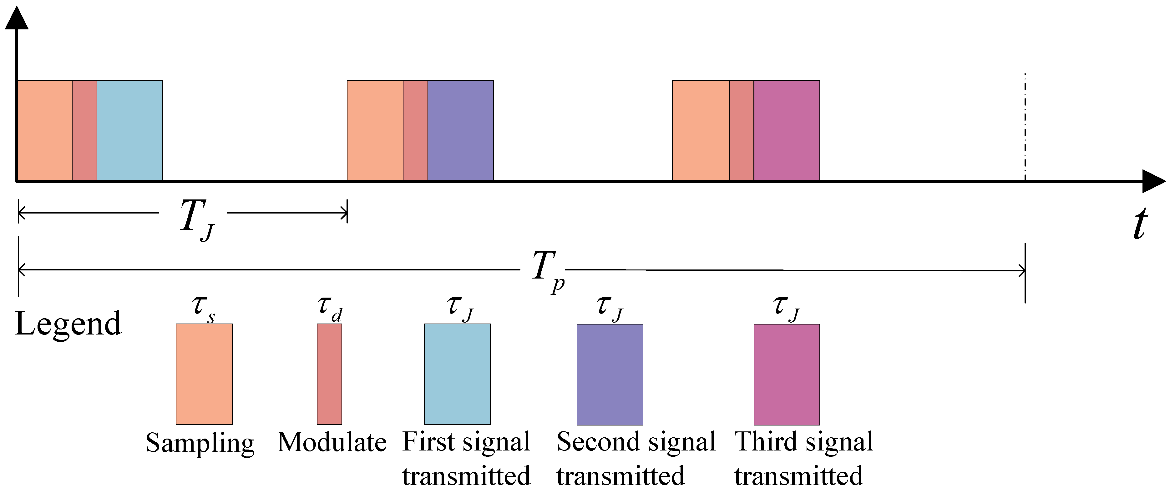
From a procedural perspective, intermittent sampling jamming can be classified into three phases: sampling, modulation processing, and transmission. During the sampling phase, the jammer searches and arranges the signal, then samples it. In the processing and modulation stage, the jammer modulates, stores, and delays the sampled signal to generate the jamming signal. During the transmission stage, the jammer amplifies and transmits the jamming signal. By adjusting the sampling timing, duration, delay time, and choosing suitable modulation and processing techniques, the number, strength, and spatial distribution of the jamming false targets can be regulated [26].

Mathematically, the sampling process can be modeled as a signal multiplication to characterize. Let the signal be $S\left(t\right)$, and the sampled signal be $P\left(t\right)$; then we have

$$P\left(t\right)=\mathrm{rect}\left(\frac{t}{{\tau }_J}\right)\otimes \sum _{n=-\infty }^{+\infty }\delta \left(t-n{T}_J\right)$$

(1)

where ${\tau }_J$ is the pulse width of the rectangular envelope of the disturbance (and often the sampling pulse width), and $T_J$ is the repetition period of the sampled signal. The sampled signal is

$$X\left(t\right)=P\left(t\right)S\left(t\right)$$

(2)

In terms of modulation processing style, intermittent sampling jamming can be divided into three categories: intermittent sampling direct jamming, intermittent sampling repeater jamming, and intermittent sampling cyclic jamming [27,28]. A visual illustration of the intermittent sampling direct jamming is presented in Figure 1.

The mathematical expression of intermittent sampling direct jamming is shown in Equation (3); ${\tau }_s$ is the sampling time and ${\tau }_d$ is the processing time.

$$X_{\mathrm{direct}}\left(t\right)=X\left(t-{\tau }_s-{\tau }_{\mathrm{d}}\right)$$

(3)

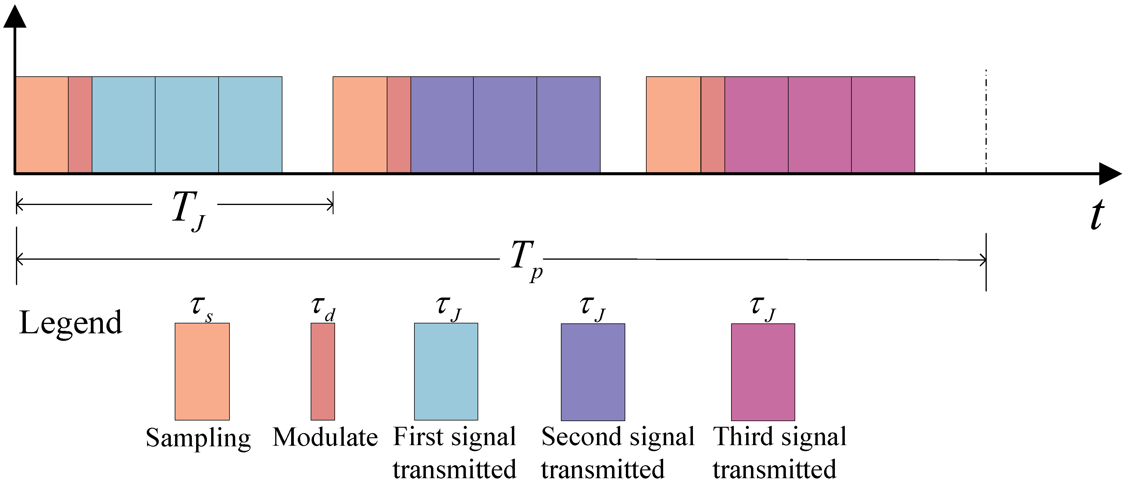
To enhance the duty cycle of intermittent sampling jamming, which is hampered by low duty cycles due to direct jamming, the sampled signal can be relayed multiple times within an interference repetition cycle rather than just once. The maximum allowable number of relays can be determined as

$$H=⌊\frac{T_J-{\tau }_s-{\tau }_{\mathrm{d}}}{{\tau }_J}⌋=⌊\frac{T_w}{{\tau }_J}⌋$$

(4)

$T_w$ is the actual length of time available for forwarding in an interference cycle $T_J$; that is, $T_J=T_w+{\tau }_{\mathrm{d}}+{\tau }_s$. This gives the signal form of intermittent sampling repeater jamming as

$$X_{\mathrm{repeat}}=\sum _{i=0}^{H-1}{X}_{\mathrm{direct}}\left(t-i{\tau }_J\right)$$

(5)

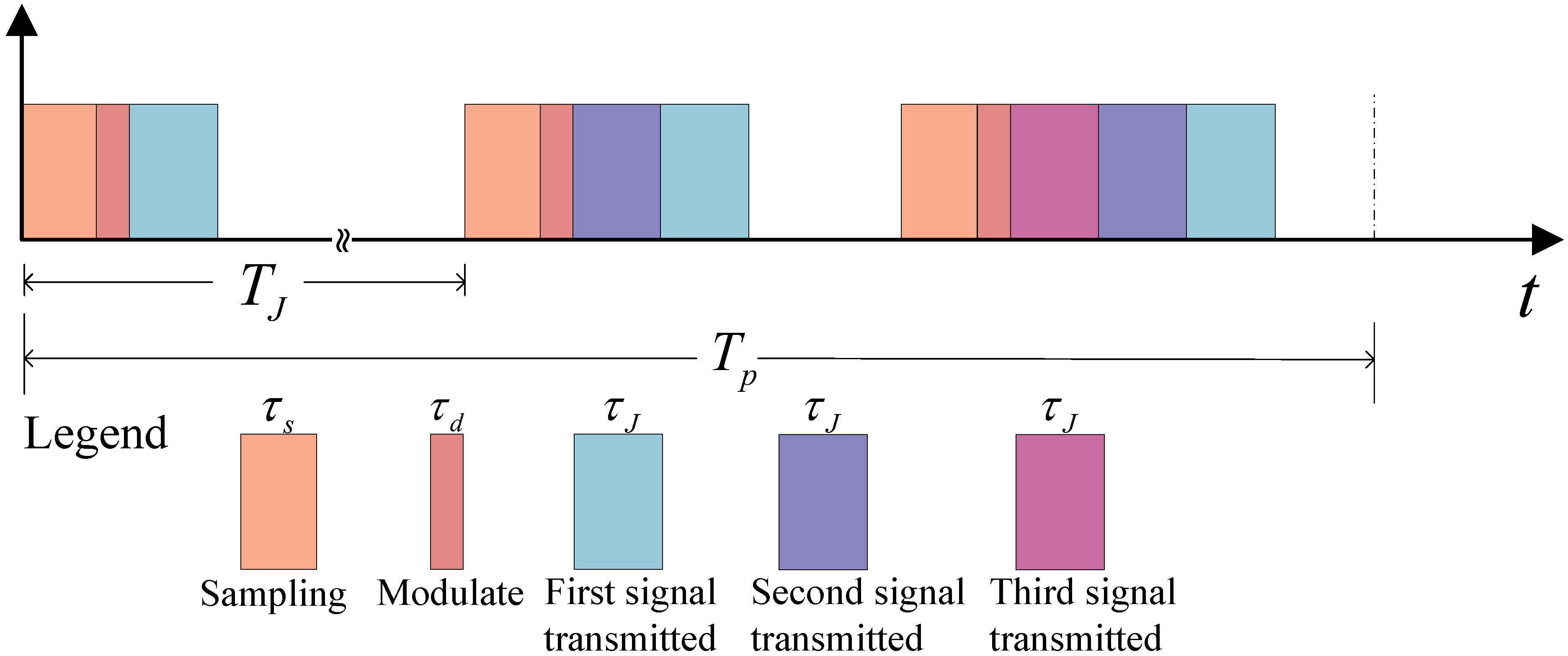
A visual illustration of the intermittent sampling repeater jamming is presented in Figure 2. Building upon this concept, it is feasible to incorporate not only a repeat of the current signal but also the previously sampled signal into the forwarded signal, thereby implementing intermittent sampling cyclic jamming. Figure 3 depicts the typical reconnaissance, interference timing, and modulation pattern of intermittent sampling cyclic jamming. In this instance, the interfering signal can be formulated as

$$X_{\mathrm{loop}}=\sum _{i=0}^{Z-1}{X}_{\mathrm{direct}}\left[t-i\left(T_J+{\tau }_J\right)\right]$$

(6)

$Z=\min \left\{G,H\right\}$, $G=⌊\frac{T_p}{T_J}⌋+1$, $T_p$ is the pulse width of the radar transmit signal, and G is the number of interference cycles within each pulse repetition cycle.

3. Description of the Proposed Method

3.1. Model of the Intra-Pulse Randomly Coded Quadrature FM and Inter-Pulse Phase Coherence Waveform

Let the radar transmit N pulses; each pulse has a pulse width of $\tau$ and a repetition period of $T_s$. There are P sub-pulses within each pulse, the operating frequency bandwidth is B, and the carrier frequency difference of P sub-pulses is an integer multiple of $\Delta f$. Then there are $⌊\frac{B}{\Delta f}⌋$ frequency bands available in the total frequency bandwidth, and for all sub-pulses, their carrier frequencies are selected by random shuffling in the above frequency bands. Then the mathematical expression of the mth sub-pulse within the nth pulse is

$$S(t,n,m)=\left\{a\left(t\right)\otimes \delta \left[t-\left(m+\frac{1}{2}\right){\tau }_{\mathrm{sub}}-n{T}_s\right]\right\}{e}^{j2\pi f_{nm}t}$$

(7)

$a\left(t\right)$ can be LFM [29] or non-LFM, pulse, phase coding, and other signals. In this paper, we only discuss LFM signals, in which case $a\left(t\right)$ can be expressed as

$$a\left(t\right)=\mathrm{rect}\left(\frac{t}{{\tau }_{\mathrm{sub}}}\right)e^{j\pi k{t}^2}$$

(8)

where ${\tau }_{\mathrm{sub}}$ is the sub-pulse pulse width, k is the FM slope, and the sub-pulse bandwidth is $B_{\mathrm{sub}}$. The LFM slope is calculated as $k=\frac{B_{\mathrm{sub}}}{{\tau }_{\mathrm{sub}}}$; $\mathrm{rect}$ (t) is a rectangular function.

$$\mathrm{rect}\left(\frac{t}{{\tau }_{\mathrm{sub}}}\right)=\left\{\begin{array}{c}1,\left|\frac{t}{{\tau }_{\mathrm{sub}}}\right|\le \frac{1}{2}\hfill \\ 0,\mathrm{else}\hfill \end{array}\right.$$

(9)

where $f_{nm}$ is the carrier frequency of the mth sub-pulse, $f_{nm}=f_c+\Delta fc(n,m)$, and $f_c$ is the initial carrier frequency. The formation of $c(n,m)$ is accomplished in the following manner. Firstly, m elements are randomly chosen from set $\left\{0,1,2,\dots ⌊\frac{B}{\Delta f}⌋\right\}$, and these m elements are strictly orthogonal in the frequency domain. Subsequently, within each pulse, the order of these m elements is shuffled and rearranged. $c(n,m)$ is also referred to as the frequency modulation coefficient of the mth sub-pulse in the nth pulse.

For the intra-pulse random quadrature FM and inter-pulse phase coherence waveform, the waveform schematic is shown in Figure 4, and the mathematical expression is

$$S\left(t\right)=\sum _{n=0}^{N-1}\sum _{m=0}^{P-1}S(t,n,m)$$

(10)

Thus, the echo signal received by the radar is $R\left(t\right)$, shown as Equation (11), where $S_r\left(t\right)$ is the target echo signal, $X_J\left(t\right)$ is the intermittent sampling jamming, and $N\left(t\right)$ is the noise signal.

$$R\left(t\right)=S_r\left(t\right)+X_J\left(t\right)+N\left(t\right)$$

(11)

As intermittent sampling jamming merely divides the transmit signal and fails to store complete pulses, certain sub-pulses are inevitably lost, posing a significant advantage for the detection of intermittent sampling jamming. In the case of the aforementioned waveform, the transmitter possesses knowledge of the frequency modulation number $c(n,m)$ of every sub-pulse. Thus, a band-pass filter can be tailored for each sub-pulse, and subsequently, the signal can be down-converted and pulse-compressed to derive the echo signal $y(t,n,m)$ of the corresponding sub-pulse, as demonstrated in Equation (12). Consequently, the interference can be identified utilizing the following algorithm.

$$y(t,n,m)=R\left(t\right)\otimes S^{*}(-t,n,m)$$

(12)

3.2. Full-Pulses and Sub-Pulses Multi-Level Maximum Inter-Class Variance Algorithm

Utilizing an intra-pulse randomly coded orthogonal FM waveform to enhance the information entropy of the transmit waveform is akin to constructing a higher-dimensional function space compared to conventional signal. The scattering process of the target and passive environment on the transmit signal is, in turn, equivalent to a linear mapping of the elements within the function space. Nevertheless, due to limitations arising from space-time constraints and detection and binning processes, the signal generated by intermittent sampling jamming corresponds to a nonlinear mapping of the elements within the function space. Upon considering the signal function’s spatial dimension, the interfering signal falls short of the necessary dimensionality, and thus, the disparity in feature dimensions can be leveraged to validate the echoes, enabling the identification and differentiation of interfering echoes.

The echo signal of the randomly coded quadrature FM waveform can be extracted by analyzing its mean, variance, moment kurtosis, and other characteristic elements within various function spaces such as the time domain, frequency domain, time-frequency domain, and fractal domain. Upon conducting a comparative study, it was observed that the variance of the sub-pulses following pulse compression serves as a differentiating factor between the target signal and intermittent sampling jamming. Additionally, the quadrature FM waveform employed in this paper encodes both intra-pulse and inter-pulse sub-pulses, resulting in slight differences in the variance of the three types of intermittent sampling jamming. Thus, the variance of the sub-pulses following pulse compression can be utilized to distinguish between the target signal and the three types of interference with precision.

The OTSU algorithm is a widely used image segmentation algorithm that selects the optimal threshold to maximize inter-class variance and minimize intra-class variance, reducing the probability of misclassification [30,31,32]. The multi-layer OTSU algorithm is an extension of the OTSU algorithm that divides data into multiple classes [33,34,35], rather than just two, with the same aim of minimizing intra-class variance and maximizing inter-class variance.

In this paper, the full-pulses multilevel maximum interclass variance algorithm and the sub-pulses multilevel maximum interclass variance algorithm are proposed based on the multilayer OTSU algorithm, specifically for the waveforms used in the study. The algorithm categorizes the variance of the absolute values of each sub-pulse after pulse compression to maximize the variance between classes. Hence, there are two concepts of “variance” here: one as the input to the algorithm and the other as the objective function of the algorithm. The procedure for the full-pulses multilevel maximum interclass variance algorithm is as follows:

1.

The absolute value of the time domain variance of the $n(n=1,2,\dots ,N)$th sub-pulse of the $p(p=1,2,\dots ,P)$th echo signal of the four echoes after pulse compression is denoted as $\mathrm{var}{(n,p)}_{\mathrm{target}}$, $\mathrm{var}{(n,p)}_{\mathrm{straight}}$, $\mathrm{var}{(n,p)}_{\mathrm{reapet}}$, and $\mathrm{var}{(n,p)}_{\mathrm{loop}}$, and these data are arranged from small to large into a one-dimensional array $\mathrm{Var}$ of size $4NP$;

2.

Assume that the first level threshold $T_1$ is chosen as the ith data $\mathrm{Var}\left(i\right)$ of the array $\mathrm{Var}$, and the second and third level thresholds $T_2$, $T_3$ are the jth data $\mathrm{Var}\left(j\right)$ of $\mathrm{Var}$ and the kth data $\mathrm{Var}\left(k\right)$ of $\mathrm{Var}$, and $i<j<k<4NP$, such that the array can be divided into four subintervals, $g_1$, $g_2$, $g_3$, and $g_4$, respectively;

3.

Calculate the probability of occurrence of each subinterval, denoted as:

$$w_1=\frac{i}{4NP}$$

(13)

$$w_2=\frac{j-i}{4NP}$$

(14)

$$w_3=\frac{k-j}{4NP}$$

(15)

$$w_4=\frac{4NP-k}{4NP}$$

(16)

4.

Calculate the average amplitude of the four intervals and the total interval:

$${\lambda }_1=\frac{{\displaystyle \sum _{h=1}^i}\mathrm{Var}\left(h\right)}{i}$$

(17)

$${\lambda }_2=\frac{{\displaystyle \sum _{h=i+1}^j}\mathrm{Var}\left(h\right)}{j-i}$$

(18)

$${\lambda }_3=\frac{{\displaystyle \sum _{h=j+1}^k}\mathrm{Var}\left(h\right)}{k-j}$$

(19)

$${\lambda }_4=\frac{{\displaystyle \sum _{h=k+1}^{4NP}}\mathrm{Var}\left(h\right)}{4NP-k}$$

(20)

$$\lambda =\frac{{\displaystyle \sum _{h=1}^{4NP}}\mathrm{Var}\left(h\right)}{4NP}$$

(21)

5.

Define the interclass variance as:

$${\sigma }^2=\sum _{h=1}^4{w}_h{\left(\lambda -{\lambda }_h\right)}^2$$

(22)

6.

Iterating over the threshold $T_1$ to $T_3$ (satisfying $T_1$ < $T_2$ < $T_3$) such that the maximum inter-class variance ${\sigma }^2$ is the optimal threshold:

$$\left\{{T_1}^{*},{T_2}^{*},{T_3}^{*}\right\}=\arg \underset{T_1<T_2<T_3}{\max }{\sigma }^2$$

(23)

Theflowchart of the full-pulses multilevel maximum interclass variance algorithm is shown in Figure 5.

The full-pulses multilevel maximum interclass variance algorithm considers all sub-pulses for threshold determination, which is effective for distinguishing between target signals and intermittent sampling jamming, but may not perform well when differentiating between different types of intermittent sampling jamming. This is because the quadrature FM waveform used in this paper varies significantly between sub-pulses, and the different types of intermittent sampling jamming also have different impacts on sub-pulses. If the same threshold is applied to all sub-pulses, misclassification of the types of interference is likely to occur. Therefore, to address this issue, differential thresholds can be set for different sub-pulses. Based on this approach, a sub-pulses multilevel maximum interclass variance algorithm is proposed, and the schematic diagram of the algorithm is illustrated in Figure 6.

4. Analysis of the Proposed Method

To validate the proposed method described in the paper, theoretical analysis and simulation experiments are conducted on the proposed waveform and the intermittent sampling jamming under this waveform. Hence, a meticulous analysis is performed in the time domain, time-frequency domain, frequency domain, and pulse compression domain to examine the characteristics of the intra-pulse random orthogonal and inter-pulse coherent frequency-modulated waveform signal, as well as three types of intermittent sampling jamming signals.

Table 1. Theparameters of the waveform and jamming.

Parameter	Value	Parameter	Value
$T_p$	41 $\mathsf{\mu }$s	B	400 MHz
${\tau }_J$	1 $\mathsf{\mu }$s	$B_{\mathrm{sub}}$	10 MHz
${\tau }_{\mathrm{d}}$	0.2 $\mathsf{\mu }$s	$\Delta f$	40 MHz
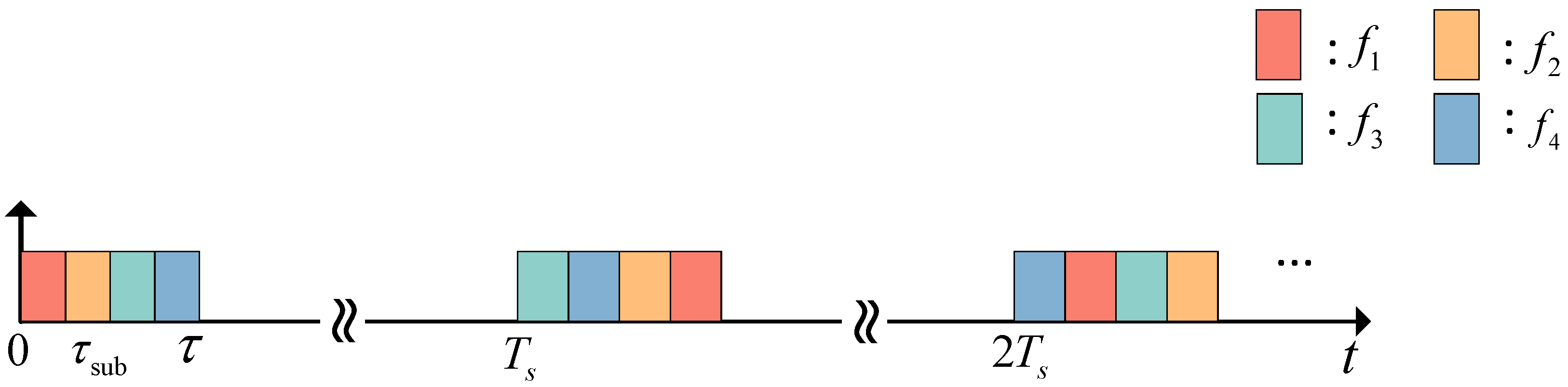
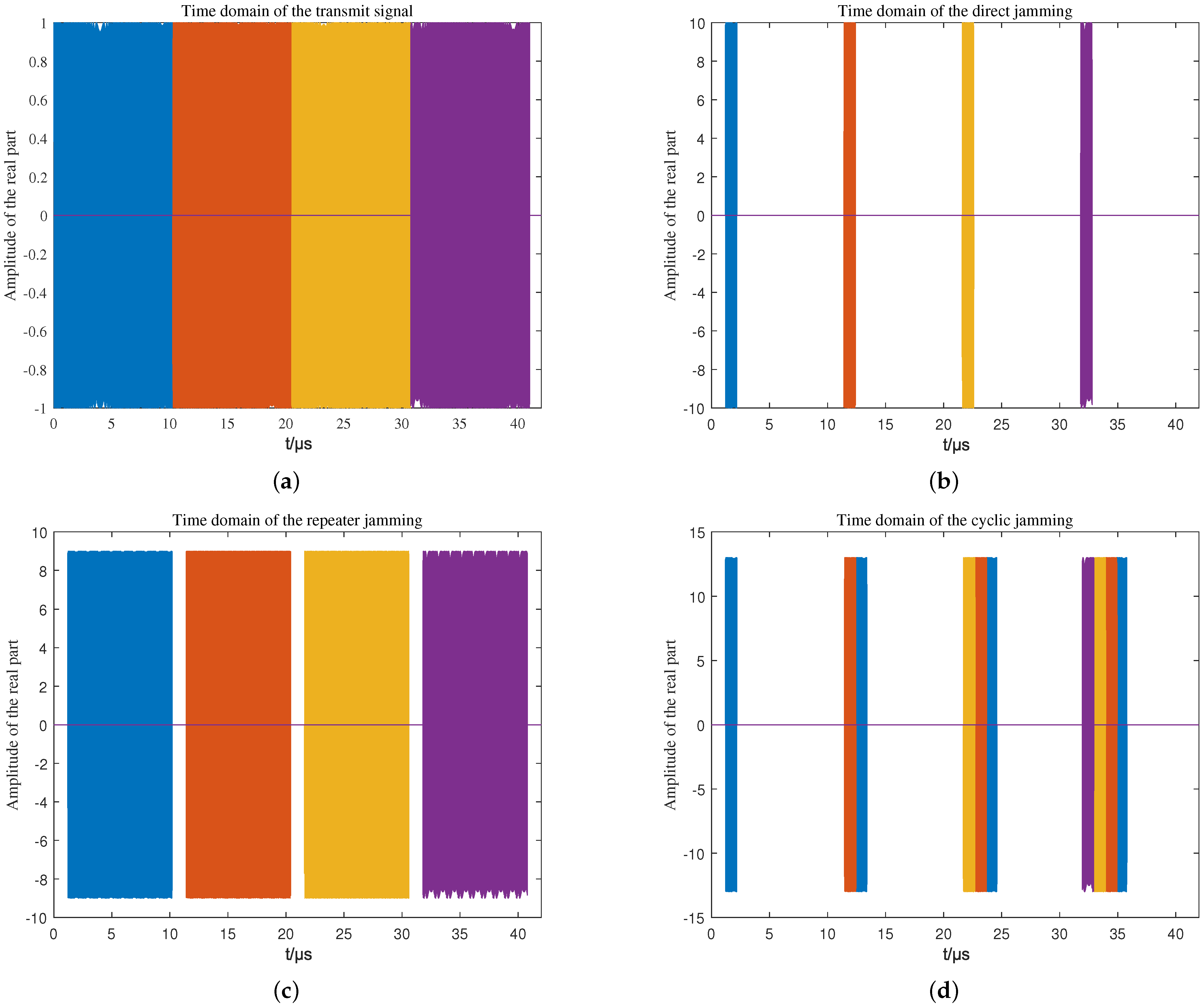
$T_J$	10.2 $\mathsf{\mu }$s	P	4

displays the parameters of the waveform utilized in the experiment. The radar system operates at a carrier frequency of 3 GHz in the S-band, with a pulse width of 41 $\mathsf{\mu }$s and a pulse repetition period of 1 ms. The experiment consists of a total of 10 pulses, with each pulse containing 4 sub-pulses. The sub-pulse bandwidth is set at 10 MHz, resulting in a total operating frequency bandwidth of 400 MHz, with a frequency interval of 40 MHz for each hop. The interference pulse width is 1 $\mathsf{\mu }$s, with an interference time delay of 0.2 $\mathsf{\mu }$s, and an interference repetition period of 10.2 $\mathsf{\mu }$s.

4.1. Time Domain Analysis and Simulation

Before conducting the time domain simulation experiments, let us delve into the difference between the signal and the three types of interference in the time domain from a theoretical point of view. A more in-depth study of the time domain expression of the emitted signal waveform is carried out according to Equation (7):

$$\begin{array}{cc}S\left(t\right)\hfill & =\sum _{n=0}^{N-1}\sum _{m=0}^{P-1}\left\{\mathrm{rect}\left(\frac{t}{{\tau }_{\mathrm{sub}}}\right)e^{j\pi k{t}^2}\otimes \delta \left[t-\left(m+\frac{1}{2}\right){\tau }_{\mathrm{sub}}-n{T}_s\right]\right\}{e}^{j2\pi f_{nm}t}\hfill \\ \hfill & =\sum _{n=0}^{N-1}\sum _{m=0}^{P-1}\left\{\underset{-\infty }{\overset{+\infty }{\int }}\mathrm{rect}\left(\frac{u}{{\tau }_{\mathrm{sub}}}\right)e^{j\pi k{u}^2}\delta \left[t-u-\left(m+\frac{1}{2}\right){\tau }_{\mathrm{sub}}-n{T}_s\right]du\right\}{e}^{j2\pi f_{nm}t}\hfill \\ \hfill & =\sum _{n=0}^{N-1}\sum _{m=0}^{P-1}\exp \left\{j\pi k{\left[\mathrm{t}-n{T}_s-\left(m+\frac{1}{2}\right){\tau }_{\mathrm{sub}}\right]}^2+j2\pi f_{nm}t\right\}\mathrm{rect}\left[\frac{t-n{T}_s-\left(m+1/2\right){\tau }_{\mathrm{sub}}}{{\tau }_{\mathrm{sub}}}\right]\hfill \end{array}$$

(24)

Hence, the $S\left(t\right)$ signal is composed of P linearly frequency-modulated sub-pulses with different carrier frequencies within each pulse. Each sub-pulse has a width of ${\tau }_{\mathrm{sub}}$. By utilizing Equations (2) and (3), we can derive the time domain expression of the intermittent sampling direct relay interference as follows:

$$\begin{array}{cc}X\left(t\right)\hfill & =\left\{\mathrm{rect}\left(\frac{t}{{\tau }_J}\right)\otimes {\displaystyle \sum _{n=-\infty }^{+\infty }}\delta \left(t-n{T}_J\right)\right\}S\left(t\right)\hfill \\ \hfill & =\left[{\displaystyle \underset{-\infty }{\overset{+\infty }{\int }}}\mathrm{rect}\left(\frac{u}{{\tau }_j}\right){\displaystyle \sum _{n=-\infty }^{+\infty }}\delta \left(t-u-n{T}_J\right)du\right]S\left(t\right)\hfill \\ \hfill & ={\displaystyle \sum _{n=-\infty }^{+\infty }}\mathrm{rect}\left(\frac{t-n{T}_J}{{\tau }_j}\right)S\left(t\right)\hfill \end{array}$$

(25)

Therefore, intermittent sampling direct jamming corresponds to the temporal interception of the transmitted signal $S\left(t\right)$ with a width of ${\tau }_j$ and a period of $T_J$. Intermittent sampling repeater jamming and intermittent sampling cyclic jamming both stem from intermittent sampling direct jamming.The time domain simulation plot is as follows.

From Figure 7, we can observe that within one pulse period, there are four sub-pulses with different carrier frequencies, each marked with a corresponding color. The characteristics of intermittent sampling repeater jamming are particularly evident in the plot, especially in the case of the interference signal for the fourth sub-pulse (indicated by the color purple), which undergoes H repetitions. Additionally, it can be observed that intermittent sampling cyclic jamming not only relays the currently intercepted sub-pulse signal but also relays past intercepted sub-pulse signals. This cyclic relay of past intercepted sub-pulse signals can generate multiple coherent false target echoes in the radar system, which will be analyzed in detail in the subsequent pulse compression analysis.

4.2. Time-Frequency Domain Analysis and Simulation

The analysis in the time-frequency domain builds upon the foundation of frequency domain analysis. According to Equation (24), we can determine the phase of each sub-pulse as follows:

$$\mathsf{\Phi }\left(t\right)=\pi k{\left[\mathrm{t}-n{T}_s-\left(m+\frac{1}{2}\right){\tau }_{\mathrm{sub}}\right]}^2+2\pi f_{nm}t$$

(26)

The phase is a quadratic function of time. Taking the derivative of the phase with respect to time, we can obtain the instantaneous frequency as follows:

$$f\left(t\right)=\frac{1}{2\pi }\frac{d\mathsf{\Phi }\left(t\right)}{dt}=kt+f_{nm}$$

(27)

It is evident that the frequency is a linear function of time. Therefore, the frequency range corresponding to each sub-pulse is $\left[f_{nm}-\frac{B_{\mathrm{sub}}}{2},f_{nm}+\frac{B_{\mathrm{sub}}}{2}\right]$, and the bandwidth for each sub-pulse is $B_{\mathrm{sub}}$. This corresponds to the concept of sub-pulse segmentation filtering discussed in Section 3.2. Therefore, when setting the hopping frequency and total bandwidth, it is necessary to ensure that the frequencies of each sub-pulse do not overlap to extract each sub-pulse without losing information in the spectrum. This lays the foundation for subsequent signal identification and processing.

Regarding the interference, according to Equation (25), we can infer that the phase of the interference signal is approximately the same as the transmitted signal. However, since the interference signal only intercepts a portion of the transmitted signal, its bandwidth is $B_j=k{\tau }_j$.

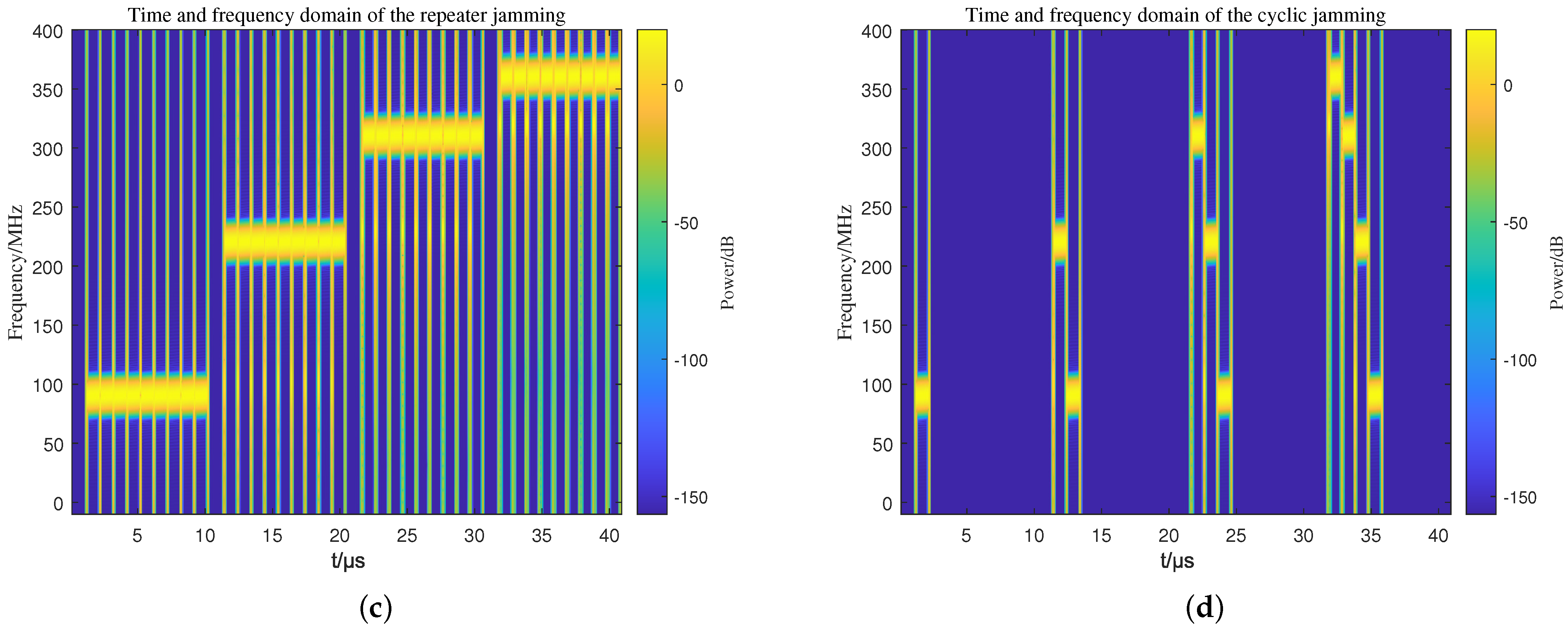
From Figure 8, it can be observed that the intermittent sampling repeater jamming exhibits a relatively continuous pattern in the time-frequency domain. Therefore, distinguishing between the target echo signal and intermittent sampling repeater jamming based on signal continuity in the time-frequency domain is not very effective. As introduced in Section 1, signal and intermittent sampling jamming identification in the time-frequency domain is more effective for low-duty intermittent sampling direct jamming and more challenging for high-duty intermittent sampling repeater jamming.

It is clear that the intermittent sampling cyclic jamming corresponds to a forwarding period of $T_J+{\tau }_J$ and a forwarding count of G for the interfering sub-signal within a signal pulse width, which aligns with Equation (6).

4.3. Frequency Domain Analysis and Simulation

According to Section 4.1, by applying the Fourier transform to the time domain signals, we can explore the distinctions between the signal and the three types of interference in the frequency domain.

$$\begin{array}{cc}S\left(f\right)\hfill & =F\left\{\sum _{n=0}^{N-1}\sum _{m=0}^{P-1}\exp \left[j\pi k{\left(\mathrm{t}-n{T}_s-\left(m+\frac{1}{2}\right){\tau }_{\mathrm{sub}}\right)}^2+j2\pi f_{nm}t\right]\mathrm{rect}\left[\frac{t-n{T}_s-\left(m+1/2\right){\tau }_{\mathrm{sub}}}{{\tau }_{\mathrm{sub}}}\right]\right\}\hfill \\ \hfill & =\sum _{n=0}^{N-1}\sum _{m=0}^{P-1}F\left\{\exp \left[j\pi k{\left(\mathrm{t}-n{T}_s-\left(m+\frac{1}{2}\right){\tau }_{\mathrm{sub}}\right)}^2+j2\pi f_{nm}t\right]\mathrm{rect}\left[\frac{t-n{T}_s-\left(m+1/2\right){\tau }_{\mathrm{sub}}}{{\tau }_{\mathrm{sub}}}\right]\right\}\hfill \\ \hfill & =\sum _{n=0}^{N-1}\sum _{m=0}^{P-1}S(f,n,m)\hfill \end{array}$$

(28)

Let F denote the Fourier transform. According to the nature of the Fourier transform as a linear transform, we can infer that the spectrum of each transmitted pulse signal is the summation of the spectra of all sub-pulses. Let $t_0=\left(m+\frac{1}{2}\right){\tau }_{\mathrm{sub}}$; we can obtain

$$\begin{array}{cc}S(f,n,m)\hfill & =F\left\{\exp \left[j\pi k{\left(\mathrm{t}-t_0\right)}^2+j2\pi f_{nm}t\right]\mathrm{rect}\left[\frac{\mathrm{t}-t_0}{{\tau }_{\mathrm{sub}}}\right]\right\}\hfill \\ \hfill & =\underset{-\infty }{\overset{+\infty }{\int }}\exp \left[j\pi k{\left(\mathrm{t}-t_0\right)}^2+j2\pi f_{nm}t\right]\exp (-j2\pi ft)\mathrm{rect}\left[\frac{\mathrm{t}-t_0}{{\tau }_{\mathrm{sub}}}\right]dt\hfill \\ \hfill & =\underset{-\infty }{\overset{+\infty }{\int }}\mathrm{rect}\left[\frac{\mathrm{t}-t_0}{{\tau }_{\mathrm{sub}}}\right]\exp \left[j\pi k{\left(\mathrm{t}-t_0\right)}^2+j2\pi f_{nm}t-j2\pi ft\right]dt\hfill \\ \hfill & =\underset{-\infty }{\overset{+\infty }{\int }}A\left(t\right)\exp \left[j\theta \left(t\right)\right]dt\hfill \end{array}$$

(29)

where $A\left(t\right)=\mathrm{rect}\left[\frac{\mathrm{t}-t_0}{{\tau }_{\mathrm{sub}}}\right]$, $\theta \left(t\right)=\pi k{\left(\mathrm{t}-t_0\right)}^2+2\pi f_{nm}t-2\pi ft$.

$A\left(t\right)$ represents the real envelope, while $\theta \left(t\right)$ represents the signal modulation phase. In comparison to the phase, the envelope is a slowly varying function of time. According to the principle of stationary phase [36,37,38], for a rapidly changing signal in the time domain, apart from the positions where the derivative is zero (stationary points), the positive and negative areas in the remaining regions almost cancel each other out. As a result, the integral of the function is primarily influenced by the stationary point regions. Now, let us solve for the stationary points:

$${\theta }^{\prime }\left(t\right)=\frac{d\theta \left(t\right)}{dt}=2\pi kt+2\pi f_{nm}-2\pi f$$

(30)

Thus, the stationary point is $t_k=\frac{f-f_{nm}}{k}+t_0$, and then the Taylor expansion [39,40] is performed for $\theta \left(t\right)$ in the vicinity of $t_k$:

$$\begin{array}{cc}\theta \left(t\right)\hfill & =\theta \left(t_k\right)+{\theta }^{\prime }\left(t_k\right)(t-t_k)+\frac{{\theta }^{″}\left(t_k\right)}{2}{\left(t-t_k\right)}^2+O\left({\left(t-t_k\right)}^2\right)\hfill \\ \hfill & =\theta \left(t_k\right)+\frac{{\theta }^{″}\left(t_k\right)}{2}{\left(t-t_k\right)}^2+O\left({\left(t-t_k\right)}^2\right)\hfill \end{array}$$

(31)

where ${\theta }^{″}\left(t\right)=\frac{d{\theta }^{\prime }\left(t\right)}{dt}=2\pi k$.

By neglecting higher-order terms beyond the second order and applying the Fresnel integral theorem [41,42], the expression can be simplified as follows:

$$\begin{array}{cc}S(f,n,m)\hfill & =A\left(t_k\right)\exp \left[j\theta \left(t_k\right)\right]\underset{t_k-\delta }{\overset{t_k+\delta }{\int }}\exp \left[j\frac{{\theta }^{″}\left(t_k\right)}{2}{\left(t-t_k\right)}^2\right]dt\hfill \\ \hfill & =\frac{1}{\sqrt{k}}\mathrm{rect}\left(\frac{f-f_{nm}}{B_{\mathrm{sub}}}\right)\exp \left[-j\pi \frac{{\left(f-f_{nm}\right)}^2}{k}\right]\exp \left[-j2\pi \left(f-f_{nm}\right)t_0\right]\exp \left(j\frac{\pi }{4}\right)\hfill \end{array}$$

(32)

where $\delta$ represents an infinitesimal quantity.

Therefore, from Equation (32), the envelope of $S(f,n,m)$ resembles a rectangle with a width distribution of $\left[f_{nm}-\frac{B_{\mathrm{sub}}}{2},f_{nm}+\frac{B_{\mathrm{sub}}}{2}\right]$. This corresponds to the frequency spectrum bandwidth of the m-th sub-pulse of the n-th pulse, which is consistent with the previous theoretical analysis.

On the basis of Equation (2), for intermittent sampling direct jamming, the spectrum is

$$\begin{array}{cc}X\left(f\right)\hfill & =F\left(P\left(t\right)S\left(t\right)\right)\hfill \\ \hfill & =F\left(P\left(t\right)\right)\otimes \mathcal{F}\left(S\left(t\right)\right)\hfill \\ \hfill & =F\left[\mathrm{rect}\left(\frac{t}{{\tau }_J}\right)\otimes \sum _{n=-\infty }^{+\infty }\delta \left(t-n{T}_J\right)\right]\otimes S\left(f\right)\hfill \\ \hfill & ={\tau }_j{f}_J\sum _{n=-\infty }^{+\infty }Sa\left(\pi {\tau }_j{f}_{J}n\right)\delta \left(f-n{f}_J\right)\otimes S\left(f\right)\hfill \\ \hfill & ={\tau }_j{f}_J\sum _{n=-\infty }^{+\infty }Sa\left(\pi {\tau }_j{f}_{J}n\right)S(f-n{f}_J)\hfill \end{array}$$

(33)

where $f_J=\frac{1}{T_J}$ is the sampling frequency of the interference, $Sa\left(x\right)=\frac{\sin \left(x\right)}{x}$.

From Equation (33), it can be observed that the spectrum of intermittent sampling direct jamming is a periodic replication of the transmit signal, weighted by the amplitude and with a weight factor of ${\tau }_j{f}_{J}Sa\left(\pi {\tau }_j{f}_{J}n\right)$. The replication period is $f_J$. The spectral analysis of intermittent sampling repeater jamming and cyclic jamming is similar to this, and the following simulations are performed to compare.

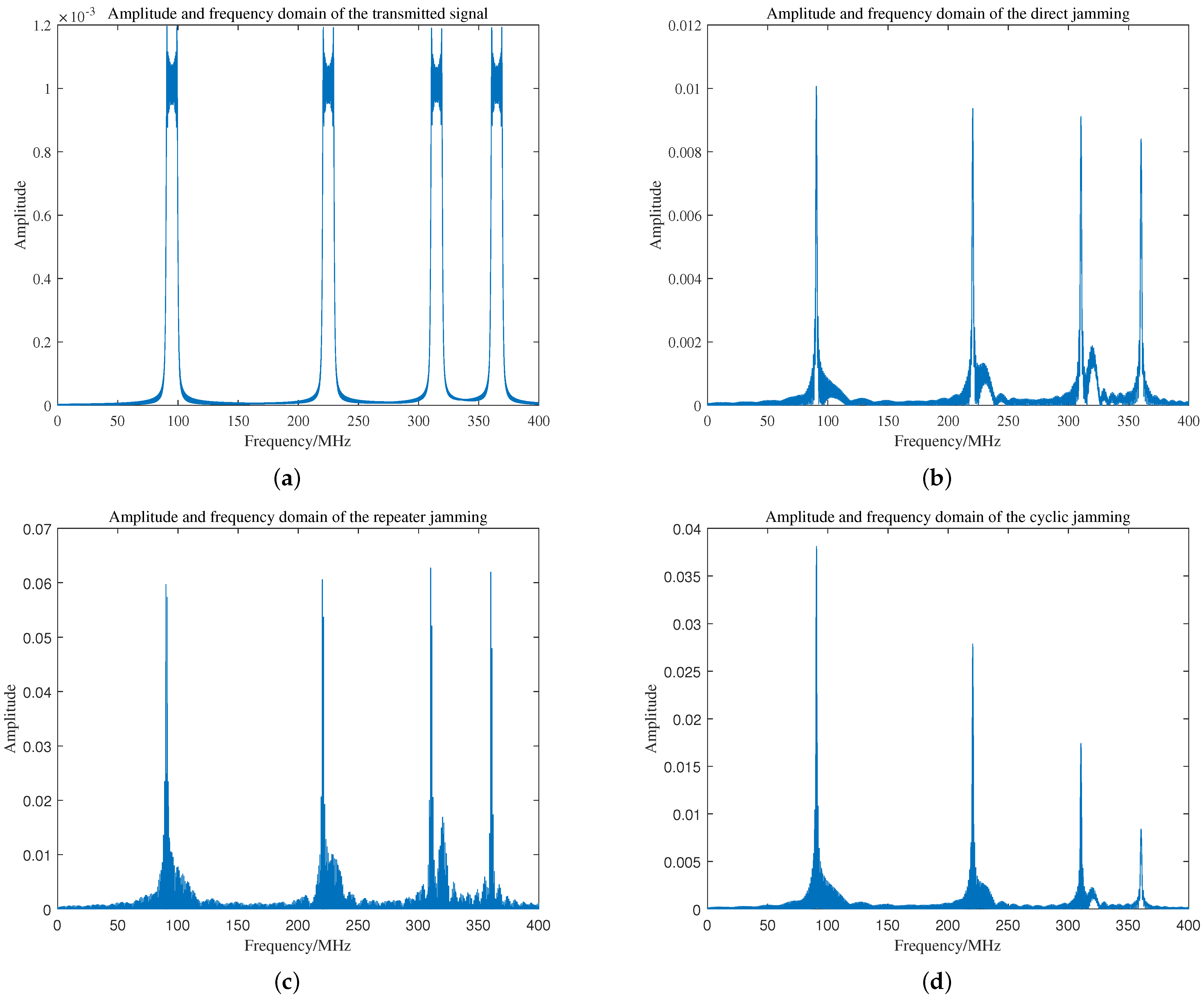
From Figure 9, we can see that the carrier frequencies corresponding to the four sub-pulses of the original signal are 90 MHz, 210 MHz, 310 MHz, and 360 MHz, respectively. The bandwidth of each sub-pulse is 10 MHz, which is $B_{\mathrm{sub}}$. It is evident from the figure that the spectral bandwidths of intermittent sampling direct jamming, repeater jamming, and cyclic jamming are similar to the radar’s transmitted signal. This spectral overlap enables highly effective interference to the radar target echoes in the frequency domain. However, due to the fact that the intermittent sampling jamming is a truncation of the transmitted signal, its spectral side lobes are significantly higher and the main lobe is widened. Moreover, in the frequency domain, there is a clear distinction between the target signal and the three types of intermittent sampling jamming, but the differences among the three interference types are relatively small.

4.4. Pulse Compression Domain Analysis and Simulation

In the above experiments, we can validate the simulation experiments through theoretical analysis, revealing that the distinction between the target signals and the three types of intermittent sampling jamming is inadequate in the time domain, time-frequency domain, and frequency domain when employing the waveform incorporating intra-pulse random orthogonal coded frequency modulation and inter-pulse phase coherence.

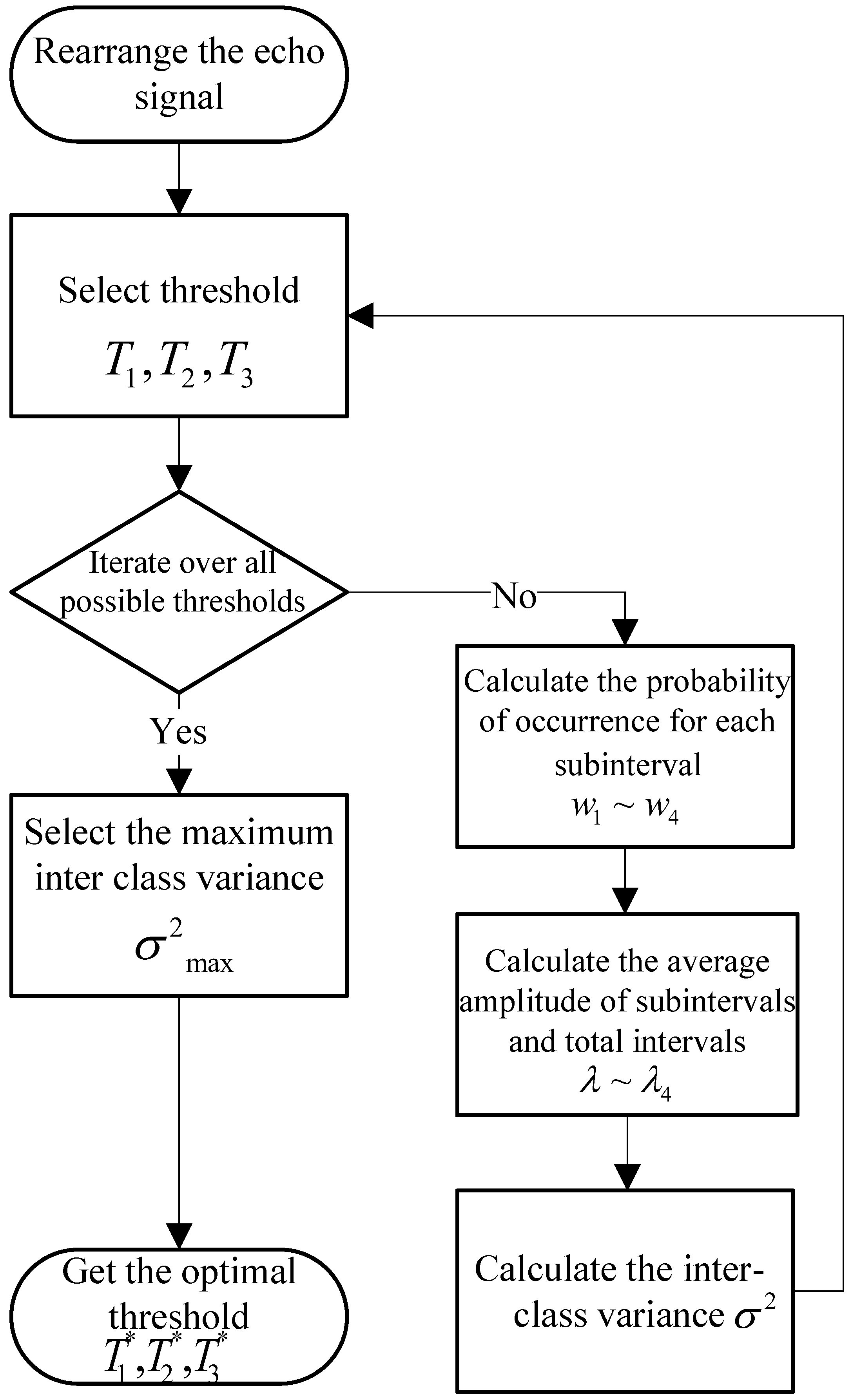
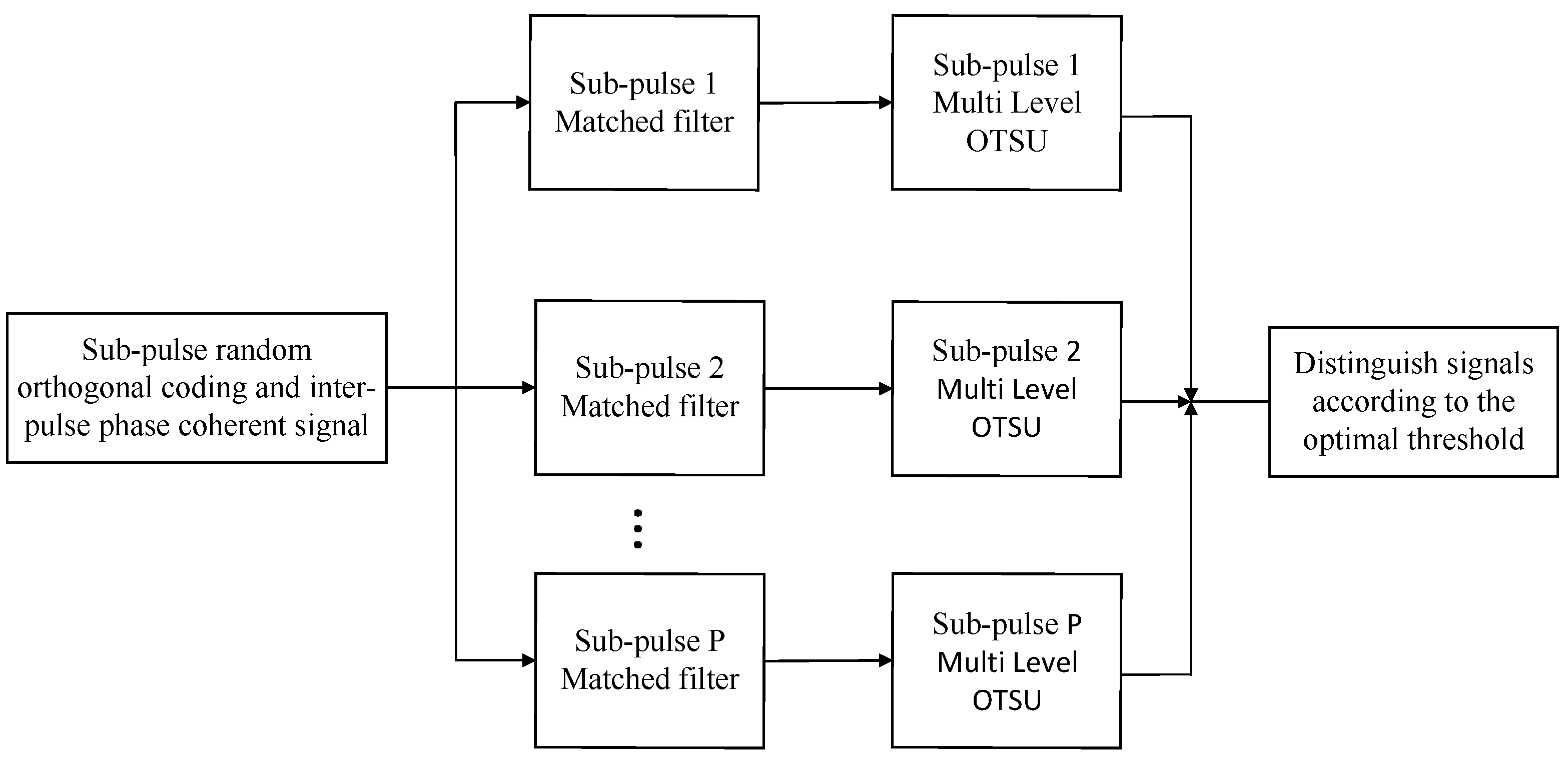
Therefore, it is crucial to conduct theoretical analysis and experimental verification of the transmitted signal and the three types of intermittent sampling jamming in the pulse compression domain. After pulse compression, the differences between the transmitted signal and the interference can be clearly manifested. Thus, the variance of each sub-pulse after pulse compression can serve as a discriminant. In this study, the proposed Full-Pulse Multilevel Maximum Inter-class Variance algorithm and Sub-Pulse Multilevel Maximum Inter-class Variance algorithm are utilized to analyze their effectiveness in discriminating between targets and interference.

As the frequency bands of different sub-pulses are orthogonal to each other, in signal processing, different filters are constructed for each sub-pulse based on their corresponding modulation index ($c\left(n,m\right)$). Then, the echoes of these sub-pulses are individually pulse-compressed. In this case, we can fix the pulse number (n) and sub-pulse number (m) for analysis. For the sake of demonstration, let us consider n = m = 0. According to Equation (24), we have

$$S\left(t\right)=\mathrm{rect}\left[\frac{t-{\tau }_{\mathrm{sub}}/2}{{\tau }_{\mathrm{sub}}}\right]\exp \left\{j\pi k{\left[\mathrm{t}-\frac{{\tau }_{\mathrm{sub}}}{2}\right]}^2+j2\pi f_{0}t\right\}$$

(34)

Then the filter corresponding to pulse compression is

$$h\left(t\right)=S^{*}(-t)=\mathrm{rect}\left[\frac{-t-{\tau }_{\mathrm{sub}}/2}{{\tau }_{\mathrm{sub}}}\right]\exp \left\{-j\pi k{\left[\mathrm{t}+\frac{{\tau }_{\mathrm{sub}}}{2}\right]}^2+j2\pi f_{0}t\right\}$$

(35)

The result of pulse compression is

$$\begin{array}{cc}{S}_0\left(t\right)\hfill & =h\left(t\right)\otimes S\left(t\right)\hfill \\ \hfill & =\underset{-\infty }{\overset{+\infty }{\int }}\mathrm{rect}\left[\frac{-u-{\tau }_{\mathrm{sub}}/2}{{\tau }_{\mathrm{sub}}}\right]\exp \left\{j\pi k{\left[\mathrm{u}+\frac{{\tau }_{\mathrm{sub}}}{2}\right]}^2+j2\pi f_{0}u\right\}\hfill \\ \hfill & *\mathrm{rect}\left[\frac{t-u-{\tau }_{\mathrm{sub}}/2}{{\tau }_{\mathrm{sub}}}\right]\exp \left\{j\pi k{\left[t-u-\frac{{\tau }_{\mathrm{sub}}}{2}\right]}^2+j2\pi f_0(t-u)\right\}du\hfill \\ \hfill & =\frac{\sin \left[\pi kt{\tau }_{\mathrm{sub}}\left(1-\frac{\left|t\right|}{{\tau }_{\mathrm{sub}}}\right)\right]}{\pi kt}\exp \left(j2\pi f_{0}t\right)\hfill \end{array}$$

(36)

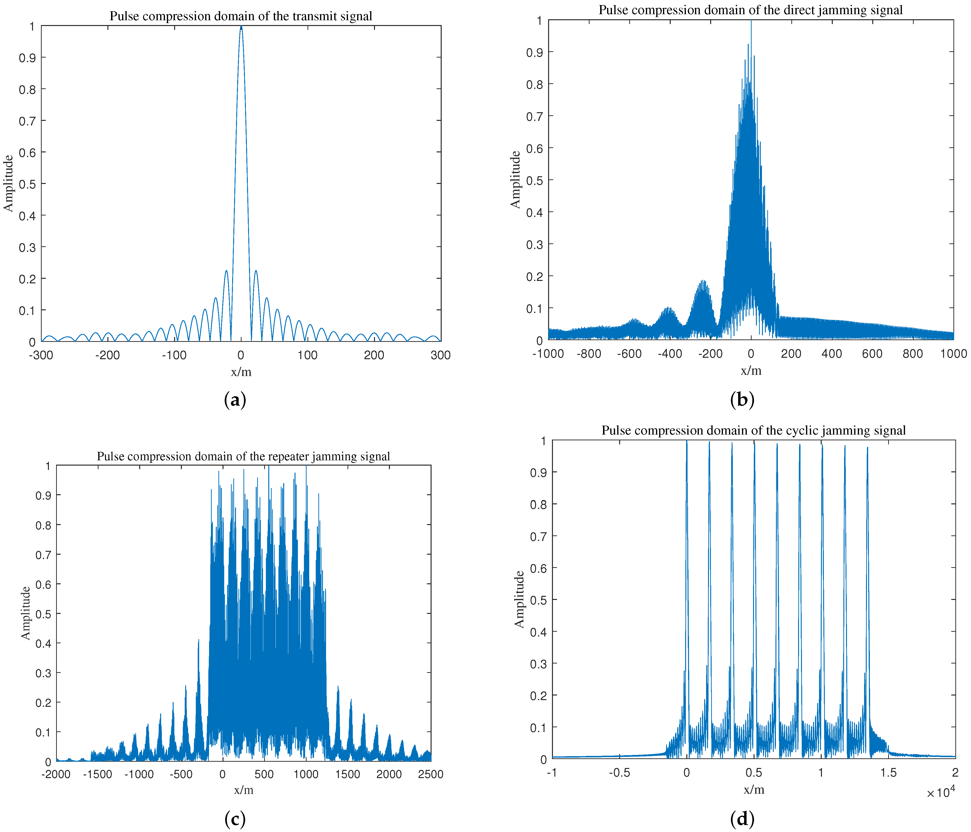
The envelope of the pulse compression result is approximately ${\tau }_{\mathrm{sub}}Sa\left[\pi B_{\mathrm{sub}}t\right]$. When $\pi B_{\mathrm{sub}}t=\pm \pi$, we can obtain $t=\pm \frac{1}{B_{\mathrm{sub}}}$. This is the first zero point, that is, the interval between the first zero points is $\frac{2}{B_{\mathrm{sub}}}$. For intermittent sampling direct jamming, a similar derivation can lead to its pulse compression envelope expression as ${\tau }_{j}Sa\left[\pi B_{j}t\right]$; likewise, the interval between its first zero points is $\frac{2}{B_j}$. Intermittent repeater forwarding interference and intermittently cyclic forwarding interference both involve forwarding the interfering sub-pulses of the intermittent direct interference with different repetitions and time delays. Therefore, the differences between the signal and the three types of interference after pulse compression can be verified through simulation.

From Figure 10, it can be observed that the distance interval between the first zero crossings of the target echo sub-pulses after pulse compression is approximately 30 m, which corresponds to a time interval of 0.2 $\mathsf{\mu }$s. This is consistent with the theoretical analysis of interval $\frac{2}{B_{\mathrm{sub}}}$. On the other hand, the first zero crossing interval of the intermittent sampling direct jamming is approximately 300 m, which matches the theoretical analysis of interval $\frac{2}{B_j}$.

The spacing between the false targets generated by intermittent sampling repeater jamming is approximately 150 m, which corresponds to a time interval of 1 $\mathsf{\mu }$s. This is just the interference pulse width ${\tau }_j$. This correspondence is consistent with Figure 8, as during repeater jamming, each interference sub-pulse is delayed by ${\tau }_j$ compared to the previous one. Therefore, the repetition period corresponds to ${\tau }_j$, and due to the close proximity of each dummy target, the sidelobes overlap during pulse compression, resulting in wider sidelobes with higher amplitudes. Similarly, the interval between dummy targets generated by intermittent sampling cyclic jamming is approximately 1680 m, or 11.2 $\mathsf{\mu }$s, which is just one interference period plus the interference pulse width, denoted as $T_J+{\tau }_j$. Additionally, due to the relatively larger separation between each dummy target, the mutual influence of sidelobes is reduced.

This observation reveals that under this waveform, there exist significant distinctions among the target echo signal, intermittent sampling direct jamming, intermittent sampling repeater jamming, and intermittent sampling cyclic jamming after pulse compression. Consequently, the variance obtained after pulse compression can be utilized for classification, serving as the fundamental basis for the Full-Pulse Multilevel Maximum Inter-class Variance algorithm.

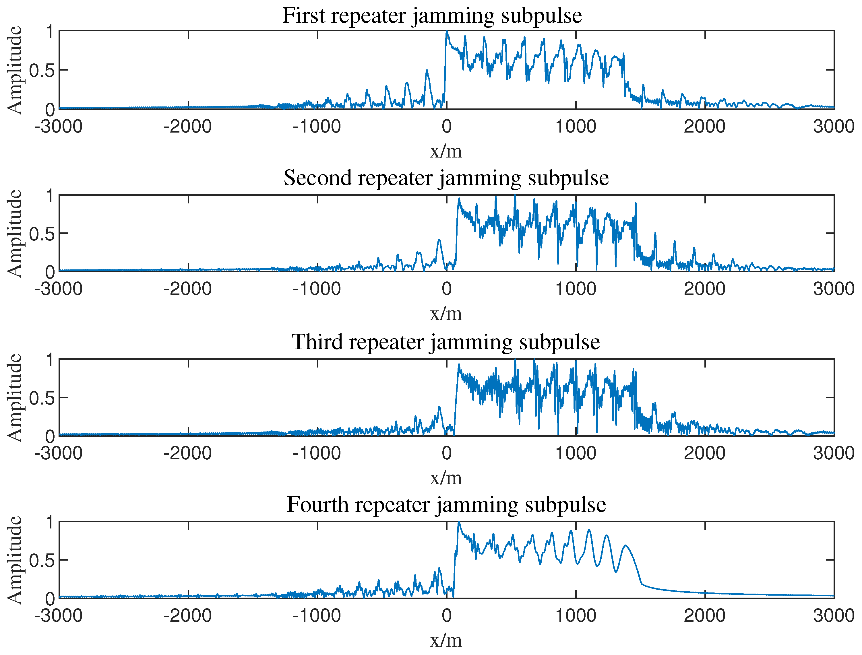
Furthermore, from Figure 11, it is evident that the pulse compression results of intermittent sampling repeater jamming vary among different sub-pulses. In fact, due to the changing relationship between interference and signal in terms of period and pulse width, the effects generated by intermittent sampling jamming differ within each sub-pulse. Therefore, it is possible to perform signal classification separately within each sub-pulse, which forms the fundamental basis of the Sub-Pulses Multilevel Maximum Inter-class Variance algorithm.

5. Echo Certification Simulation Experiment and Analysis

Based on Section 4, we set the number of radar transmitting pulses N to 10, sub-pulse P to 8, and varied the Jamming-to-Signal Ratio (JSR) from 10 dB to 20 dB, as well as the Signal-to-Noise Ratio (SNR) from −20 dB to 20 dB after sub-pulse matched filtering. The simulation analyzed the recognition accuracy of the full-pulses multilevel maximum inter-class variance algorithm and the sub-pulses multilevel maximum inter-class variance algorithm for target signal and three types of interference. The simulation was repeated 300 times using the Monte Carlo method. Figure 10 shows the results of the 300 Monte Carlo simulations when JSR is 10 dB.

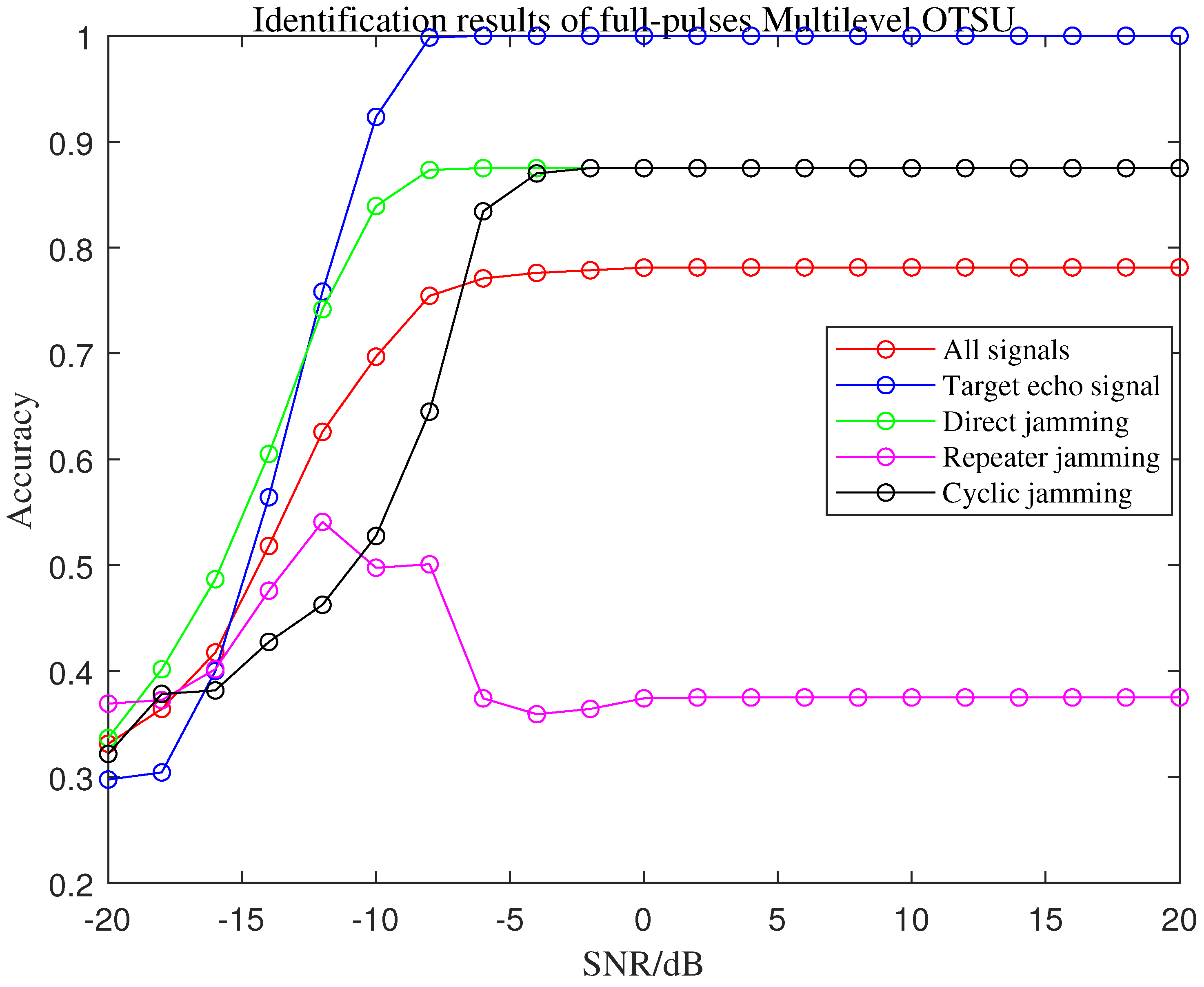
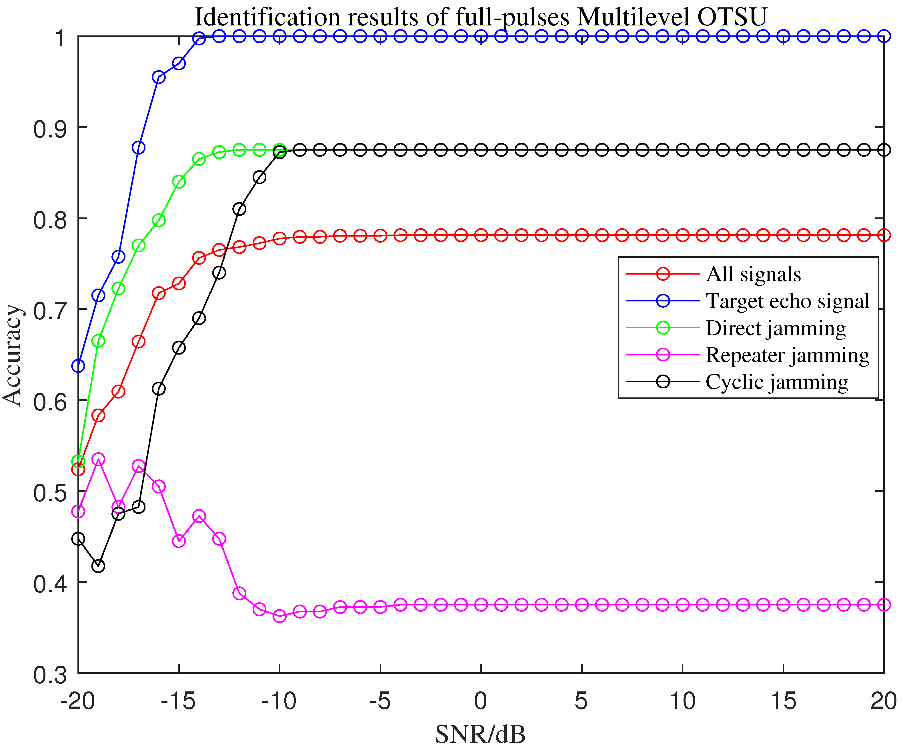
Figure 12 demonstrates that with increasing SNR after pulse compression, the recognition accuracy of the target echo signal, intermittent sampling direct jamming, and intermittent sampling cyclic jamming all improve when using the full-pulses shared thresholding algorithm. However, at low SNR levels, the algorithm primarily calculates the variance of noise undulation, leading to lower recognition accuracy.

As the SNR increases, the full-pulses shared threshold algorithm can distinguish the variances of the target and the three types of interference based on their different energy and signal undulation characteristics. The recognition accuracy of the target echo signal is stable at 100% for SNR = −5 dB, while the recognition accuracy of intermittent sampling direct jamming and intermittent sampling cyclic jamming is stable at approximately 85%. The recognition accuracy of all four signals is stable at around 78%.

However, the recognition accuracy of the full-pulses shared threshold algorithm for intermittent sampling repeater jamming is low. From Figure 11, we can observe that the interference effects vary among different sub-pulses. Therefore, if the same threshold is applied to all sub-pulses, it will inevitably lead to misclassifications. Furthermore, the variance of intermittent sampling cyclic jamming is similar to that of intermittent sampling repeater jamming, making it difficult to distinguish the subtle difference in the case of full-pulses shared thresholding. Consequently, intermittent sampling repeater jamming is often recognized as intermittent sampling cyclic jamming, as shown in the fuzzy matrix in

Table 2. Confusionmatrix for full-pulses multilevel maximum interclass variance algorithm.

Mode one	78	1	1	0
Mode two	4	70	3	3
Mode three	2	3	35	40
Mode four	4	3	0	73
	Mode one	Mode two	Mode three	Mode four

and

Table 3. Signal patterns corresponding to the confusion matrix.

Mode one	Target echo signal
Mode two	Target echo signal plus Direct Jamming
Mode three	Target echo signal plus Repeater Jamming
Mode four	Target echo signal plus Cyclic Jamming

for SNR = 0 dB.

From the results, it is clear that when 40 sub-pulses are interfered by intermittent sampling repeater jamming, they are misidentified as intermittent sampling cyclic jamming using a common threshold for all pulses. Thus, it is difficult to distinguish intermittent sampling repeater jamming from intermittent sampling cyclic jamming with a common threshold for all pulses. However, the recognition accuracy of the target echo signal is almost perfect, with a recognition accuracy close to 100%.

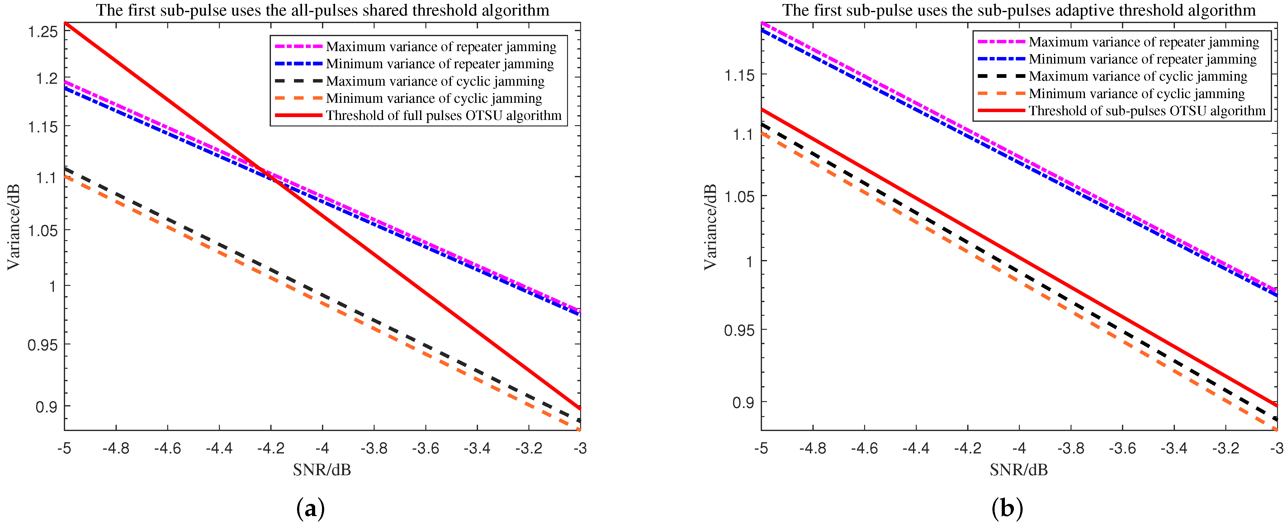
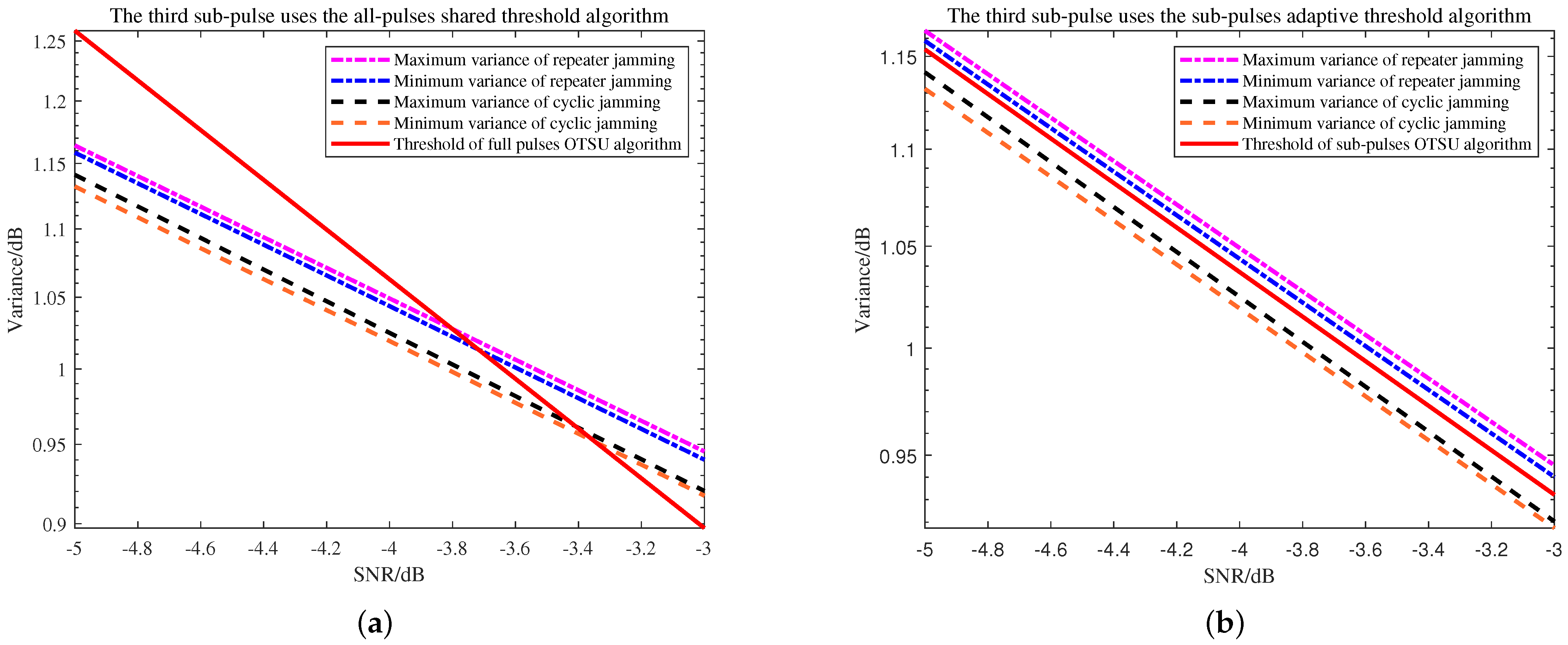
Based on the information provided in Figure 13 and Figure 14, it is evident that the intermittent sampling repeater jamming has a larger variance than the intermittent sampling cyclic jamming, which has a smaller variance. When applying the full-pulses shared threshold algorithm, it becomes clear that the two types of interference cannot be accurately distinguished at either the first or third sub-pulses, as the variance of the interferences varies across different sub-pulses. Hence, using a global threshold for all sub-pulses would result in a significant reduction in recognition accuracy. In contrast, the sub-pulses adaptive thresholding approach can effectively differentiate between the two types of interference by employing a set threshold.

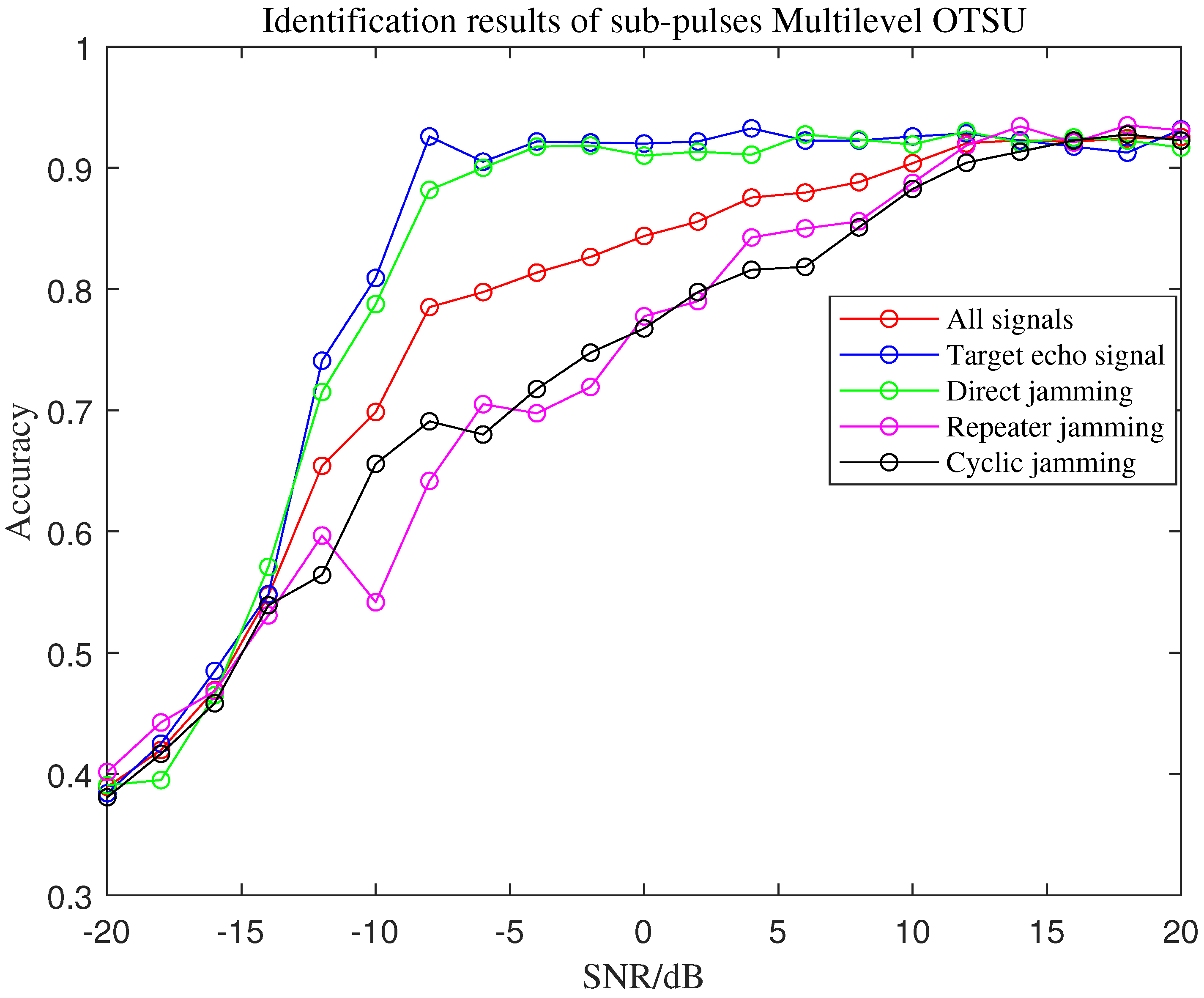
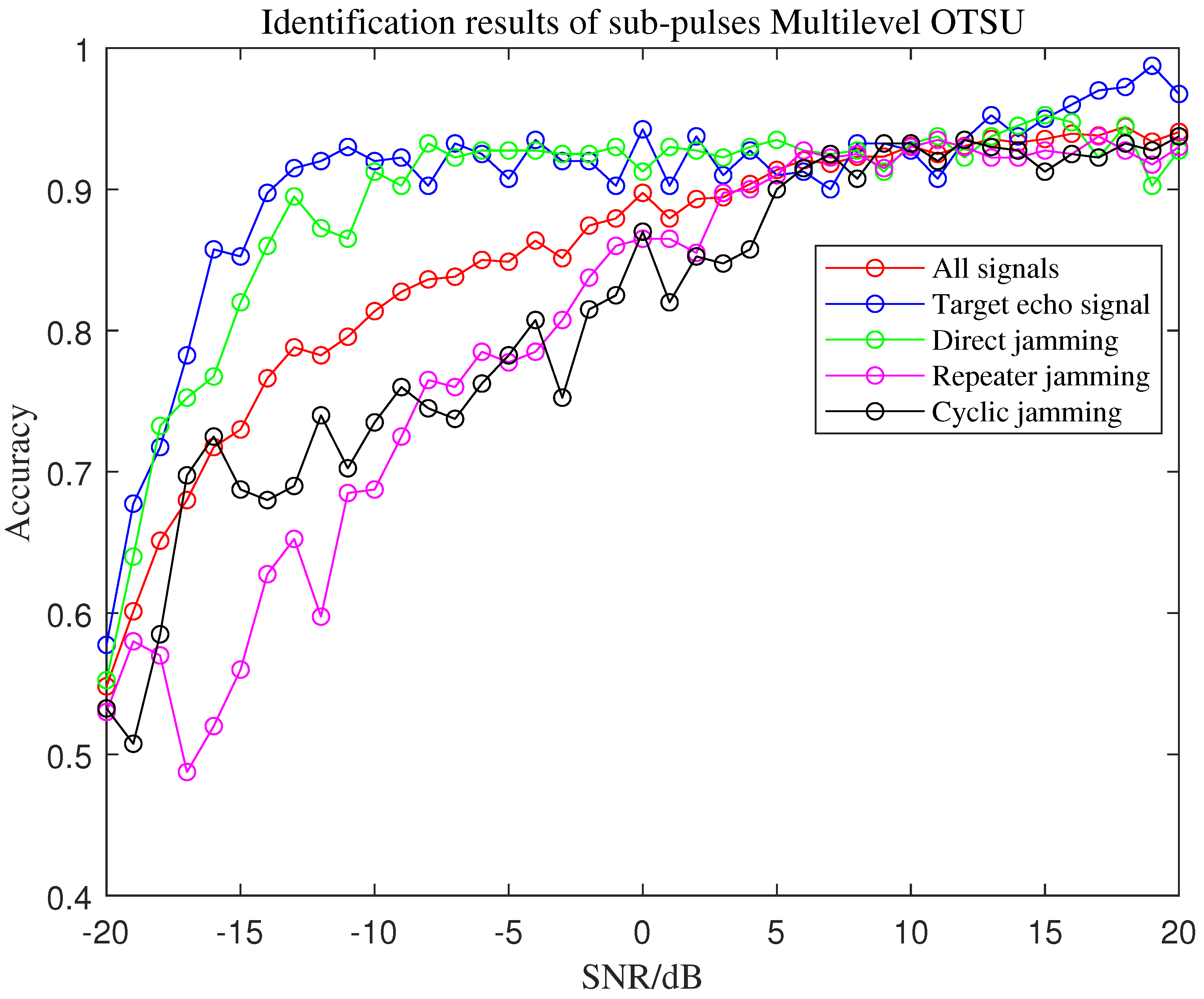
Figure 15 illustrates that the sub-pulses adaptive thresholding algorithm shows an increasing trend in recognition accuracy as SNR increases for both the signal and the three interferences, with a stabilized recognition accuracy of about 93%. It can be concluded that this algorithm has a significantly higher recognition rate for intermittent sampling repeater jamming compared to the full-pulses shared thresholding algorithm. However, due to the smaller energy and variance fluctuations of the echo signal within each sub-pulse compared to the interference, the recognition accuracy decreases compared to the full-pulses shared threshold algorithm. Overall, the sub-pulses adaptive thresholding algorithm has a higher recognition accuracy for all signals and interferences, but at the cost of a higher SNR for each sub-pulse.

The confusion matrix in

Table 4. Confusionmatrix for sub-pulses multilevel maximum interclass variance algorithm.

Mode one	75	2	2	1
Mode two	4	74	0	2
Mode three	2	3	71	4
Mode four	4	3	0	73
	Mode one	Mode two	Mode three	Mode four

indicates that the recognition rate of the target signal and the three types of interference is high, and the intermittent sampling repeater jamming and intermittent sampling cyclic jamming can be accurately distinguished.

When the JSR is increased to 20 dB, the results shown in Figure 16 and Figure 17 indicate that the SNR values of both the signal and interference decrease while the recognition accuracy remains stable, as compared to the JSR of 10 dB. This is attributed to the enhanced energy of the interference signal and more distinct variance characteristics, allowing for a stable recognition accuracy to be achieved at a lower SNR.

Based on the theoretical analysis and experimental results, it can be concluded that the proposed algorithms have demonstrated their effectiveness in identifying and distinguishing different types of interference in radar systems. The full-pulses multi-level maximum inter-class variance algorithm is capable of detecting intermittent sampling interference and the target signal with high accuracy, while the sub-pulses multi-level maximum inter-class variance algorithm is more effective in identifying the three types of intermittent sampling interference. By combining these two algorithms in cascade, it is possible to achieve highly accurate identification of the target signal and effective distinction of different types of interference in radar systems.

6. Conclusions

With the purpose of addressing the challenge pertaining to the identification of the target signal and diverse forms of intermittent sampling jamming, this paper puts forth a radar waveform that amalgamates intra-pulse random orthogonal coded frequency modulation with inter-pulse phase coherence. This waveform takes into account the functions of anti-jamming and inter-pulse coherence. Leveraging this proposed waveform, the paper introduces the full-pulses multi-level maximum inter-class variance algorithm, which exhibits a remarkable recognition rate for the target signal. When the Jamming-to-Signal Ratio (JSR) is 10 dB and the Signal-to-Noise Ratio (SNR) is −5 dB, the target recognition rate approximates 100%. Nevertheless, distinguishing between intermittent sampling repeater jamming and intermittent sampling cyclic jamming proves challenging for the algorithm. Building upon this premise, the paper enhances the algorithm and introduces the innovative sub-pulses multilevel maximum interclass variance algorithm. This algorithm further employs adaptive thresholds tailored to individual sub-pulses, thereby improving the accuracy of the recognition process. With respect to typical SNR and JSR conditions, the recognition rate for both the signal and the three types of jamming surpasses 90%. Furthermore, the algorithm’s adaptability to diverse environments enables its practical implementation in engineering. This, in turn, enhances the resistance of coherent phase radar system against intermittent sampling jamming.

In MTI and MTD radar systems, the waveform proposed in this paper can not only obtain better anti-jamming effect, but also be compatible with anti-clutter processing. Therefore, one of the forthcoming objectives of this study involves developing an effective approach to filter out intermittent sampling jamming amidst the presence of significant ground clutter. Furthermore, in this paper, the waveform is designed to vary the sub-pulse carrier frequency within the pulse and the relative order of the sub-pulses between the pulses, without further analysis of the more complex sub-pulse carrier frequency-pulse repetition period joint variation waveform. Hence, the subsequent focus will be on exploring methods to enhance the variation of the pulse repetition interval (PRI) based on the existing waveform. This enhancement aims to expand the range of speed measurement and ensure robust interference recognition capabilities.