Article

Comprehensive Ocean Information-Enabled AUV Motion Planning Based on Reinforcement Learning

1
School of Big Data and Artificial Intelligence, Guangxi University of Finance and Economics, Nanning 530003, China
2
Guangxi Big Data Analysis of Taxation Research Center of Engineering, Nanning 530003, China
3
School of Electronic Information, Guangxi Minzu University, Nanning 530006, China
4
School of Electrical and Information Engineering, Tianjin University, Weijin Road, Tianjin 300072, China
*
Author to whom correspondence should be addressed.
Remote Sens. 2023, 15(12), 3077; https://doi.org/10.3390/rs15123077
Submission received: 15 April 2023 / Revised: 6 June 2023 / Accepted: 9 June 2023 / Published: 12 June 2023
(This article belongs to the Special Issue Underwater Communication and Networking)

Abstract

:
Motion planning based on the reinforcement learning algorithms of the autonomous underwater vehicle (AUV) has shown great potential. Motion planning algorithms are primarily utilized for path planning and trajectory-tracking. However, prior studies have been confronted with some limitations. The time-varying ocean current affects algorithmic sampling and AUV motion and then leads to an overestimation error during path planning. In addition, the ocean current makes it easy to fall into local optima during trajectory planning. To address these problems, this paper presents a reinforcement learning-based motion planning algorithm with comprehensive ocean information (RLBMPA-COI). First, we introduce real ocean data to construct a time-varying ocean current motion model. Then, comprehensive ocean information and AUV motion position are introduced, and the objective function is optimized in the state-action value network to reduce overestimation errors. Finally, state transfer and reward functions are designed based on real ocean current data to achieve multi-objective path planning and adaptive event triggering in trajectorytracking to improve robustness and adaptability. The numerical simulation results show that the proposed algorithm has a better path planning ability and a more robust trajectory-tracking effect than those of traditional reinforcement learning algorithms.

1. Introduction

Covering 71% of the Earth’s surface area while being rich in material resources such as minerals, energy and organisms [1], the oceans are extremely important for both the natural ecosystem and human society. Therefore, researchers have invested much effort in researching intelligent, stable and efficient ocean exploration technologies. Among them, autonomous underwater vehicles (AUVs), as important ocean exploration technology tools, have been widely used because they have better flexibility [2] and can accomplish large-scale and wide-ranging underwater ocean monitoring [3].
To enhance the robustness and adaptability of AUV motion, numerous researchers have conducted extensive scientific research in the field of motion planning and achieved remarkable results. Motion planning research encompasses environmental modeling and motion planning algorithms. Environmental modeling necessitates the modeling of both environmental and motion models. An environmental model is utilized to establish a description of the spatial positions of an AUV object within the environment, as well as their corresponding attribute characteristics. Existing environmental modeling methods include the grid method [4], Voronoi diagrams [5], and inverse distance weighting (IDW) [6]. The environmental model established by the grid method is discrete, and actions can only be performed at grid vertices, resulting in systematic errors under actual conditions. The Voronoi diagram method maximizes the distance between the AUV and the obstacles, leading to suboptimal motion planning results. The IDW method, based on the grid method, employs distance-based similarity for weighted interpolation to address the errors caused by the discrete states in the grid method and establish a more realistic environmental model. The motion model defines the state and action outputs of the examined AUV. Traditional methods include the particle method and dynamic method [7]. The particle method simplifies AUV to a particle, while the dynamic method accurately reflects its motion based on performance. This paper uses IDW and dynamic methods for environmental modeling.
It is important to consider the motion-planning algorithms of AUV in addition to environmental modeling [8]. Motion planning algorithms are primarily utilized for path planning and trajectory-tracking tasks. The algorithm’s optimization objective in path planning tasks is to obtain the optimal path to reach the target point. Traditional algorithms include the A* algorithm [9], rapidly exploring random trees (RRT) algorithm [10], rapidly exploring random trees star (RRT*) algorithm [11], particle swarm optimization [12], ant colony optimization [13], and genetic algorithm [14]. The first three methods [9,10,11] are straightforward to implement, but their efficiencies are constrained by the scale of environmental modeling and decrease as the search range expands. The last three approaches are based on intelligent bionic models [12,13,14]. These algorithms have more advantages than the former techniques, but their ability to extract features in more complex environments is limited, resulting in poor generalization ability, a tendency to fall into local optima, and difficulty in meeting practical application requirements. Due to the influence of time-varying ocean currents, the state of the ocean environment is constantly changing, making it very difficult for these algorithms to complete path planning tasks. In trajectory-tracking tasks, the algorithm’s optimization objective is to ensure that the AUV’s motion trajectory remains as consistent as possible with the target trajectory. Traditional algorithms include nonlinear model-based predictive controllers [15,16,17] and proportional–integral–differential (PID) control [18]. Ocean currents introduce uncertainty into the AUV’s state, making it challenging for traditional algorithms to complete trajectory tracking tasks in ocean environments.
With the development of artificial intelligence (AI), increasingly complex AI technologies are being used in AUV motion planning [19], providing more possibilities for solving underwater problems using the Internet of Things [20]. Reinforcement learning (RL), as a new machine learning paradigm, learns through trial and error. The goal of an RL policy is to maximize reward values or achieve specific goals during the process of interacting with the environment [21,22]. This training process endows RL with nonmodality, flexibility, and adaptability, giving it high potential in complex and ever-changing ocean environments. In [23], a value-based Q-learning algorithm was successfully applied to obstacle avoidance tasks. However, this method requires the use of tables to store all operations, consuming considerable storage resources. Mnih et al. [24] incorporated a deep Q network (DQN), which uses deep neural networks to represent state-action value networks and addresses the curse of dimensionality. Chu et al. [25] introduced the DQN algorithm into the AUV path planning task. Zhang et al. [26] incorporated deep deterministic policy gradient (DDPG) [27] into the AUV trajectory-tracking tasks, reducing the induced tracking errors. Du et al. [28] and Hadi et al. [29] used twin delayed deep deterministic policy gradient (TD3) [30] as the AUV state control method to obtain better results, but the exploration process of the algorithm is slow. Xu et al. [31] and Huang et al. [32] introduced soft actor–critic (SAC) [33] for AUV path planning, improving the algorithm’s exploration ability; however, nly single tasks were considered. He et al. [34] proposed asynchronous multithreading proximal policy optimization (AMPPO) based on proximal policy optimization (PPO) [35], which achieved good results in multiple task scenarios, but the designs of the individual environments used the experiment were relatively simple. In present studies [25,26,28,29,31,32,34] on modeling reinforcement learning environments, the real ocean current data are seldom considered, and the overestimation error caused by the ocean current is rarely taken into account in these algorithms, which leads to the low exploration rate, poor adaptability, and robustness in motion planning. To solve these problems, a reinforcement learning-based motion planning algorithm based on comprehensive ocean information (RLBMPA-COI) is proposed to AUV motion planning tasks. The main contributions of this paper are as follows:
  • To create a realistic ocean current environment, the AUV motion model and real ocean current data are introduced into the environment modeling based on reinforcement learning. This method effectively minimized the distance between practical applications and the simulations. Therefore, this method brings more significant practical value to AUV motion planning.
  • We proposed the RLBMPA-COI AUV motion planning algorithm based on a real ocean environment. By incorporating local ocean current information into the objective function of the action-value network, this algorithm successfully minimizes the overestimation error interference and enhances the efficiency of motion planning. According to the influence of the ocean current, target distance, obstacles, and steps on the motion planning task, we also established a corresponding reward function. This ensures the efficient training of the algorithm, further improving its exploration ability and better adaptability.
  • Multiple simulations, including complex obstacles and dynamic multi-objective tasks in path planning, as well as a trajectory-tracking task are designed to verify the performance of the proposed algorithms comprehensively. Compared with state-of-art algorithms, the performance of RLBMPA-COI has been evaluated and proven by numerical results, which demonstrate efficient motion planning and high flexibility for expansion into different ocean environments.
The remainder of this paper is organized as follows. Section 2 introduces the AUV motion model, ocean current model and SAC background information. Then, we describe the specific method implementation details in detail in Section 3. In Section 4, we discuss a variety of experiments to verify the performance of the algorithm. Finally, we conclude our work in Section 5.

2. Background

2.1. AUV Motion Model

As the carrier of the algorithm, the motion model of an autonomous underwater vehicle (AUV) is crucial. An AUV has six degrees of freedom (DOFs). The motion model of an AUV is illustrated in Figure 1, which displays both the ground-fixed coordinate system and the body axis coordinate system of the AUV [7]. Both systems follow the right-hand rule. In the ground-fixed coordinate system, the state vector of an AUV η = [ x , y , z , σ , β , χ ] represents its three-axis position and rotation information. In contrast, within the body axis coordinate system, v = [ u , v , w , g , h , j ] corresponds to the velocity and angular velocity of each directional component.
The kinematic equations of the AUV are derived by transforming the motion vector v in the body axis coordinate system into a global state vector η in the ground-fixed coordinate system.
η = T v 0 0 T w v
T v = cos β cos χ cos σ sin χ + sin σ sin β cos χ sin σ sin χ + cos σ sin β cos χ cos β sin χ cos σ cos χ + sin σ sin β sin χ sin σ cos χ + cos σ sin β sin χ sin β sin σ cos β cos σ cos β
T w = 1 tan β sin σ tan β cos σ 0 cos σ sin σ 0 sin σ cos 1 β cos ϕ cos 1 β

2.2. Ocean Current Modeling

The changing conditions of an ocean environment are influenced by a combination of factors that are time-varying and uncertain. Among them, ocean currents are the key factors affecting AUV motion planning. For this reason, many scholars have conducted research related to ocean current models. One of the more common methods for constructing ocean current models is functional simulation. For example, Ref. [36] described an ocean current model as follows:
C u r x = k 1 C u r max sin ( k 3 y ) cos ( k 3 y ) + k 1 cos ( 2 k 1 t ) + k 4 C u r y = λ C u r max cos ( k 2 x ) sin ( k 3 y ) + k 5
In this model, the latitude and longitude velocity components are represented by C u r x and C u r y , respectively. The variables k 1 , k 2 , k 3 , and λ are related to the underwater environment and may change with factors such as tides and depth. The variables k 4 and k 5 are random variables that reflect the variability of the underwater environment. In an actual ocean environment, the vertical velocity component of a 3D currents is much smaller than the longitudinal component and is often neglected for simplicity.
However, a functional simulation model is limited by its input parameters and may not accurately reflect real ocean currents. Utilizing such a model as an ocean current environment may reduce realism and limit its practical use. The meanings of the model symbols are also shown in Table A1.

2.3. Soft Actor–Critic

In this study, we apply reinforcement learning (RL) to solve the AUV motion planning problem in a continuous state action space. To implement a deep RL algorithm in the continuous space, we first defined a tuple S , A , p , r based on a Markov decision process. Assuming that the state space S and action space A are continuous, the state transition probability p ( s t , s t + 1 , a t ) : S × S × A [ 0 , ) is expressed as the probability density of the next state s t + 1 S , given the current state s t S and action a t A . Additionally, we use ρ π s t and ρ π s t , a t to denote the trajectory distribution of the state and state-action probabilities under policy π a t | s t .
For conventional RL, the optimization goal is to maximize the expected value of the strategy π a t | s t , that is:
π nor = arg max π t E ( s t , a t ) ρ π [ r ( s t , a t ) ]
However, to ensure that the developed RL algorithm can fully explore the environment and avoid becoming trapped in a local optimal solutions, an entropy term H ( π ( | s t ) is incorporated into the policy. This improves the exploration capability of the RL algorithm, allowing it to explore the environment more quickly while avoiding local optima. The policy π E nt corresponding to the maximum entropy of RL is as follows:
π E nt = arg max π t E ( s t , a t ) ρ π [ r ( s t , a t ) + α t H ( π ( | s t ) ) ]
α t is an adaptive temperature parameter that specifies the relative importance of the entropy term in the reward function. This controls the stochasticity of the optimal policy and thus the degree of exploration. The temperature coefficient is initially set to a relatively large value to ensure sufficient exploration during the early stages of training. The adaptive temperature parameter α t 0 is then adjusted to ensure that the algorithm gradually stabilizes during the later stages of training.

3. Methods

The ocean environment is constantly changing and remains uncertain due to the impact of ocean currents on AUV motion. To achieve improved adaptability and intelligence, the algorithm needs to adjust to changes in the ocean currents. Therefore, we designed a comprehensive ocean information-enabled AUV motion planning model based on RL (RLBMPA-COI) to effectively suppress the disturbances caused by ocean currents in AUV motion planning.

3.1. Marine Environmental Information Model

To balance the simplicity and realism of the environmental simulation and reduce the discrepancy between the simulated and actual environments, this study utilizes real ocean data to construct a time-varying ocean current model and improve the confidence level of the AUV motion planning environment. We focus on the South China Sea (22.25°N to 22.75°N, 115.50°E to 116°E) and use data from the National Data Center for Marine Science [37,38]. We constructed a comprehensive time-varying ocean current model using various information such as temperature, wind speed, wave intensity, wave temperature, and salinity from January to June 2021. The vertical velocity of a 3D ocean current is much smaller than its longitude and latitude components and is usually ignored to reduce the complexity of environmental simulation.
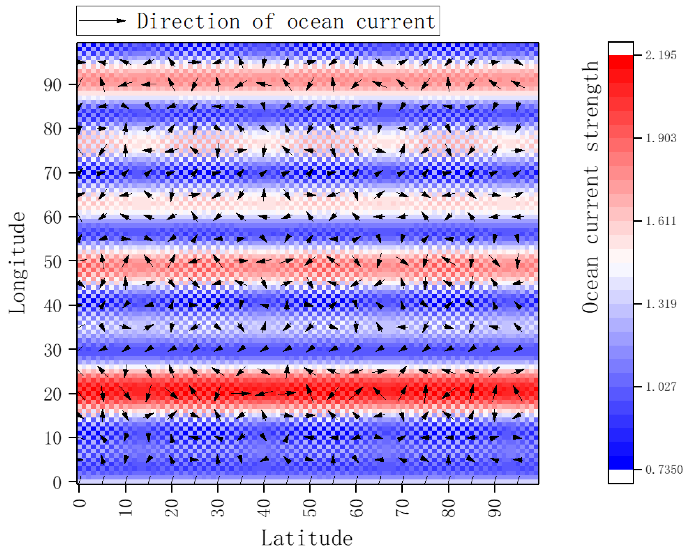
This study constructs an ocean simulation environment based on real ocean environment data using the GYM framework. The GYM framework is a reinforcement learning environment framework developed by the OpenAI company, and it has been widely used in the field of reinforcement learning. First, a grid method is used to create a 100 × 100 scale grid corresponding to the study area. Then, an inverse distance weighted interpolation method is used to interpolate the integrated ocean data model into the grid so that the AUV can obtain the ocean changing current state in a continuous space. The ocean current vector is C u r ( x t , y t ) = [ C u r x ( t ) , C u r y ( t ) ] T . The longitudinal current velocity C u r x and the latitudinal current velocity C u r y in the plane of the geostationary coordinate system O X Y are shown in Figure 2, where t corresponds to the current moment. The variation in the surface currents is shown in Figure 3, where the direction of the black arrows corresponds to the direction of the currents and the distribution of the heatmap corresponds to the current intensity C u r ( x t , y t ) . Notably, 10 grid lengths correspond to 0.05°.

3.2. Reinforcement Learning Environment

Based on the ocean current change model, an RL environment is designed, which includes two basic modules: a state transition function and a reward function. The scale of this RL environment is 100 × 100 grids, and all observation parameters and output parameters are scaled by 50 times the scale size.

3.2.1. State Transition Function

The state transition function describes the changes in the environment corresponding to the actions taken by the AUV at each moment. To reduce the computational complexity of the algorithm, we only consider the AUV motion in the horizontal plane. Correspondingly, η and v in the AUV motion model can be simplified to η = [ x , y , χ ] and v = [ u , v , j ] . The change in the position of the AUV is not only affected by its speed, but also related to the present strength of the ocean current C u r ( x t , y t ) . Therefore, the change in the state vector of the AUV can be expressed as:
x ˙ y ˙ χ ˙ = u cos 2 χ + v cos χ sin χ + C u r x u cos χ sin χ + v sin 2 χ + C u r y j
To meet the needs of motion planning tasks, two features are introduced, namely D i s o and D i s t , which represent the distance of the AUV relative to obstacles and the distance relative to the target position, respectively. Overall, the state space of this RL environment can be expressed as S = [ η , v , C u r ( x t , y t ) , D i s o , D i s t ] .
Additionally, we designed a continuous action space A so that the algorithm can take more accurate actions. Specifically, the action output consists of speed v and yaw angle δ a u v . The range of values for peed is related to the maximum ocean current speed | v | [ 0.5 C u r max , 2 C u r max ] , and the range of values for the yaw angle corresponds to the range of angles at which the hull can turn at the current moment δ a u v [ π π 4 4, π /4].

3.2.2. Reward Function

In RL, the model seeks to maximize the expected reward value, which further influences the directional gradient update process of the neural network. By combining the task requirements of path planning and trajectory tracking, this paper carefully designs the corresponding reward functions.
In the path planning task, the target reward suffers from sparsity and abrupt changes. Therefore, a distance reward r s is designed to guide the training procedure of the algorithm.
r s = min Set i = 1 n k i g o a l D i s t ( P , P i g o a l )
k i g o a l = 10 e 4 , D i s t ( P , P i g o a l ) < S t a r 1 , e l s e
k i g o a l represents reaching the target, D i s t ( P , P i g o a l ) represents the distance of the AUV relative to the target, and S t a r represents the criterion for judging whether the target has been reached. To evaluate the ability of the algorithm to adapt to ocean currents changes, an ocean current reward r c u r is designed.
r c u r = sgn ( u cos 2 χ + v cos χ sin χ C u r x u cos χ sin χ + v sin 2 χ C u r y T ) C u r ( x t , y t )
When the AUV reaches the target point, it triggers a task completion event and receives a task completion reward r g o a l .
r g o a l = 0 , i = 0 n k i ( t + 1 ) g o a l k i ( t ) g o a l = 0 200 , e l s e
When the AUV approaches or reaches the obstacle position, it triggers a collision event and receives an obstacle reward r o . The obstacle reward r o is set in levels as a warning value and a collision value, and is judged based on the obstacle warning distance S w and the obstacle collision distance S c . The obstacle collision reward r o is also affected by the completion of task D i s l .
D i s l = min Set i = 1 n k i g o a l D i s ( P o b s , P i g o a l )
r o = 0 , D i s o S w 5 , S w > D i s o S c 30 D i s l , D i s o < S c
Finally, the step reward r s t e p and the total reward r are defined. Specifically, γ c u r = 0.4 , λ s t e p = 10 e 4 . The weight of the ocean current reward is determined by the parameter γ c u r and the distance reward r s , and the weight can be adaptively adjusted to improve the adaptability and robustness of the algorithm to changes in ocean currents.
r = r s + | r s | γ c u r r c u r + r g o a l + r o λ s t e p / r s t e p
In the trajectory-tracking task, an event trigger reward r t is defined to judge the overlap of trajectories. At the same time, the distance reward r s is modified to satisfy the requirements of trajectory tracking. P t r a c e is the target position of the trajectory.
r t = 0 , D i s ( P , P t r a c e ) > S t a r 1 , e l s e
r s = D i s t ( P , P t r a c e )
r = r s + r t + γ c u r exp ( r t + r s 1 ) r c u r + r o
The total trajectory-tracking reward is r. The weight coefficient of the ocean current reward exp ( r t + r s 1 ) is adaptively adjusted to improve the robustness of tracking and the adaptability of the algorithm to ocean currents changes.

3.3. RLBMPA-COI Algorithm

In an ocean environment, ocean currents have a significant impact on the motion state of an AUV. Therefore, a motion planning algorithm for an AUV needs to fully consider the impact of ocean currents to reduce the interference caused by changes in ocean currents. To satisfy this requirement, we designed a reinforcement learning-based motion planning algorithm with comprehensive ocean information, the RLBMPA-COI algorithm. The system block diagram of this algorithm is shown in Figure 4.
Overall, the RLBMPA-COI algorithm includes a pair of state-action value networks Q θ i ( s t , a t ) , i = 1 , 2 , a pair of target state-action value networks Q θ i ( s t , a t ) , i = 1 , 2 , and a policy network π ϕ ( s t , a t ) . Their respective network parameters are θ 1 , θ 2 , θ 1 , θ 2 and ϕ . The RLBMPA-COI algorithm enhances the exploration ability of the algorithm by introducing the action entropy α t H ( π ( | s t ) , so the optimization goal of the policy network π can be expressed as:
π = arg max π t E ( s t , a t ) ρ π [ r ( s t , a t ) + α t H ( π ( | s t ) ) ]
The state-action value network Q θ i ( s t , a t ) is used to evaluate the current policy. Furthermore, it is defined as:
Q θ i ( s t , a t ) = Δ r ( s t , a t ) + γ E s t + 1 p [ V ( s t + 1 ) ] , i = 1 , 2
V ( s t ) = Δ E a t π ϕ [ Q θ i ( s t , a t ) log π ϕ ( a t | s t ) ]
V ( s t ) is the soft state-value function, and γ is a discount factor. By introducing the target state-action value networks Q θ i ( s t , a t ) to assist with training the state-action value networks Q θ i ( s t , a t ) , the training process is stabilized. In existing methods, a trimmed state-action value function y Q t a r is typically used as the target function.
y Q t a r = r ( s t , a t ) + γ min i = 1 , 2 Q θ i ( s t + 1 , π ϕ ( s t + 1 ) ) α t log π ϕ ( a t + 1 | s t + 1 )
However, y Q t ar only considers the impact of random errors on the update of the Q θ i ( s t , a t ) network and does not account for the systematic errors caused by the motion of ocean currents, which can lead to overestimation. Therefore, this paper specifically analyzes and improves the impact of ocean current motion on the training process of the Q θ i ( s t , a t ) network.
To attain improved generalization, the ocean current is simplified to sinusoidal functions C u r x and C u r y in the longitudinal and transverse components, respectively. The state-action value networks Q θ 1 and Q θ 2 can represent the state of the ocean current during sampling as follows:
Q θ 1 : C u r x 1 = B σ sin ( b σ x ) C u r y 1 = C β sin ( c β y )
Q θ 2 : C u r x 1 = B σ sin ( b σ x + Δ σ ) C u r y 1 = C β sin ( c β y + Δ β )
Different sampling moments result in phase differences between the ocean current in Q θ 1 and Q θ 2 , forming a systematic overestimation error that cannot be eliminated in y Q t ar . Assuming that the phase difference is constant, the existing overestimation error in the longitudinal direction can be defined as ε Δ σ :
ε Δ σ = 1 2 π 0 2 π min { C u r x 1 , C u r y 1 } d σ x , C u r x 1 0 , C u r y 1 0
Assuming that the sampled phase difference σ is uniformly distributed in [ 0 , 2 π ] , the average systematic overestimation error caused by the interference of the longitudinal ocean current can be calculated as ε σ :
ε σ = 0 2 π 0 2 π min { C u r x 1 , C u r y 1 } d σ x d Δ σ 2 π 2 , C u r x 1 0 , C u r y 1 0
ε σ = 1 2 π 2 0 2 π 0 2 π min { B σ sin ( b σ x ) , B σ sin ( b σ x + Δ σ ) } d σ x d Δ σ = 2 B σ 2 π 2 0 2 π 0 π σ 2 sin ( b σ x ) d σ x d ( Δ σ ) = B σ b π B σ b 2 π 2 sin ( b π ) , B σ sin ( b σ x ) 0 , B σ sin ( b σ x + Δ σ ) 0
Similarly, in the transverse direction, the average systematic overestimation error caused by the ocean current can be expressed as ε β :
ε β = C β c π C β c 2 π 2 sin ( c π )
Due to the systematic overestimation error caused by ocean currents in the reward function, this paper incorporates an ocean current reward weight coefficient q u e c u r into the experience tuple, that is, ( s t , a t , r , s t + 1 , k i g o a l , q u e c u r ) . At the same time, an ocean current weight queue Q u e c u r is designed, which can add q u e c u r to the queue and output smoothed weight values γ x and γ y . The target function y Q t a r is redefined as:
y Q t a r = r ( s t , a t ) + γ ( 1 γ x ε σ γ y ε β ) × min i = 1 , 2 Q θ i ( s t + 1 , π ϕ ( s t + 1 ) ) α t log π ϕ ( a t + 1 | s t + 1 )
We calculate the mean squared error (MSE) loss of the state-action value network.
J Q ( θ i ) = E ( s t , a t ) D [ 1 2 ( Q θ i ( s t , a t ) y Q t ar ) 2 ] = E ( s t , a t ) D [ 1 2 ( Q θ ( s t , a t ) ( r ( s t , a t ) + γ ( 1 γ x ε σ γ y ε β ) E s t + 1 p [ V θ ¯ ( s t + 1 ) ] ) ) 2 ]
The parameter θ i is optimized using the random gradient descent method:
^ θ i J Q ( θ i ) = Q θ i ( s t , a t ) r ( s t , a t ) + γ ( 1 γ x ε σ γ y ε β ) × min i = 1 , 2 Q θ ( s t + 1 , a t + 1 ) α t log ( π ϕ ( a t + 1 | s t + 1 ) ) θ i Q θ i ( s t , a t )
Finally, we update θ i : θ i θ i λ θ ^ θ i J Q ( θ i ) , i = 1 , 2 , where λ θ is the update weight. We update the target network parameters θ i : θ i θ i + ( 1 δ ) θ i , i = 1 , 2 , where δ is the soft update weight.
For the strategy network π ϕ ( a t | s t ) , the loss function is:
J π ( ϕ ) = E s t D , ε t N [ α log ( π ϕ ( f ϕ ( ε t ; s t ) | s t ) Q θ ( s t , f ϕ ( ε t ; s t ) ) ]
The action is reparametrized under the influence of the neural network a t = f ϕ ( ε t ; s t ) . The gradient corresponding to the loss function of the strategy network π ϕ ( a t | s t ) is
^ ϕ J π ( ϕ ) = ϕ α t log ( π ϕ ( a t | s t ) + ( a t α t log ( π ϕ ( a t | s t ) ) a t min i = 1 , 2 Q θ i ( s t , a t ) ) ^ ϕ f ϕ ( ε t ; s t )
Finally, we update the parameter ϕ : ϕ ϕ λ ϕ ^ ϕ J π ( ϕ ) , where λ ϕ is the update frequency. In addition, the loss function J ( α t ) dynamically adjusts the entropy weights α t :
J ( α t ) = E a t π ϕ α t log π ϕ ( a t | s t ) α t H 0
where H 0 is the target entropy and the corresponding gradient function is ^ α t J ( α t ) = log π ϕ ( α t | s t ) H 0 , while the entropy weight α t is updated by α t α t λ α t ^ α t J ( α t ) , where λ α t is the update frequency. The algorithm pseudocode is shown in Algorithm 1.    
Algorithm 1: RLBMPA-COI algorithm.
1Initialize the environment and set the number of episodes n = 0 ;
2Initialize a replay buffer D with a capacity of B r ;
3Randomly initialize the policy network π ϕ and state-action value networks Q θ i ( s t , a t ) , i = 1 , 2 with parameter vectors ϕ , θ 1 , θ 2 ;
4 Initialize the target state-action value networks Q θ 1 ( s t , a t ) with parameter vectors θ 1 θ 1 , θ 2 θ 2 ;
5Define the total training steps T, episode training steps T e p i ;
6foreach n in set T do
7    Reset the step counter for each episode t = 0 ;
8    Clear the event trigger flag r o = 0 , r t = 0 ;
9    Clear the task completion flag r g o a l = 0 ;
10    Reset the environment, AUV start point P 0 , initial state S 0 ;
11    while  t < = T e p i or not k i g o a l 10 e 4 or not r o < 5  do
12          Integrate ocean current information and AUV motion state
               s t = [ η , v , C u r ( x t , y t ) , D i s o , D i s t ] ;
13          Based on the AUV motion model and state s t , take action according to
     policy π ϕ ( s t , a t ) ;
14          if  D i s o < S c  then
15                 r o = 30 D i s l Trigger obstacle collision reward, end this episode
16          else
17                if  S w > D i s o S c  then
18                       r o = 5 , trigger obstacle warning reward
19                else
20                      pass;
21                end
22          end
23          if  D i s t < S t a r  then
24                 r t = 1 , trigger target tracking reward
25          end
26          Get an AUV state S t = [ η , v , C u r ( x t , y t ) , D i s o , D i s t ] , update the rewards
             r s , r s t e p , r c u r , and calculate the total reward r;
27          Integrate to obtain the state S t + 1 and various rewards of the next moment,
            determining the triggering of the obstacle events and target events, and
            calculate the total reward r;
28          Store the experience ( s t , a t , r , s t + 1 , k i g o a l , q u e c u r ) in D;
29           t = t + 1 ;
30    end
31     n = n + 1 ;
32    if  n % f g is True  then
33          Sample a segment of experience from D;
34          Extract the weight of the ocean current reward q u e c u r to the queue Q u e c u r ;
35          Calculate the average ocean current weight ε σ , ε β in the queue Q u e c u r ;
36          Update y Q t ar ;
37          Update θ i θ i λ θ ^ θ i J Q ( θ i ) , i = 1 , 2 ;
38          Update ϕ ϕ λ ϕ ^ ϕ J π ( ϕ ) ;
39          Update α t α t λ α t ^ α t J ( α t ) ;
40          Update θ i θ i + ( 1 δ ) θ i , i = 1 , 2 ;
41    end
42end

4. Experiments and Discussions

4.1. Basic Settings

This study focuses on a section of the South China Sea (from 22.25°N to 22.75°N and from 115.50°E to 116°E). An ocean current model is built using data from the National Ocean Science Data Center. Based on the GYM reinforcement learning framework, the model is imported into a 100 × 100 grid and expanded into a continuous simulation environment using inverse distance-weighted interpolation. Time-varying ocean current values are affected by AUV position. A complete state environment and action output space are constructed by combining the AUV motion model and ocean current model.
This study divides motion planning into path planning and trajectory tracking. We implement algorithms such as SAC, DDPG, TD3, PPO, and AMPPO. The environmental state space is partially observable and the AUV can obtain its state, current state, obstacle observation, and target position. The experiments were performed on Ubuntu 18.04 with 64 GB RAM, NVIDIA GTX3080 GPU and Python 3.8. The specific parameters of the algorithm are shown in Table A2 and Table A3.

4.2. Path Planning Tasks

4.2.1. Path Planning Task with Complex Obstacles

Given the complexity of the real ocean environment, this research concentrates on the path planning task for an AUV in ocean currents. The effectiveness of path planning is evaluated using indicators such as the number of episodes, travel distance per episode, success rate and reward value.
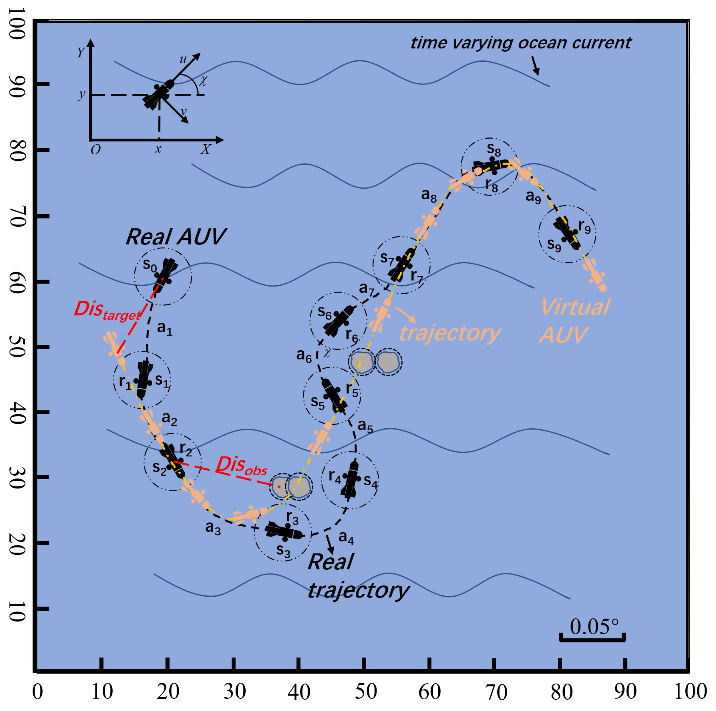
The AUV must navigate to its target location while contending with time-varying ocean currents and complex obstacles. As illustrated in Figure 5, the AUV is initialized at a fixed location at an arbitrary angle. Utilizing its current state information, it selects actions based on its policy and calculates a reward value. The AUV must adapt to changing ocean currents and use event-triggering mechanisms to perceive and avoid dense obstacles while moving toward its target location under the influence of ocean currents to maximize its cumulative rewards.
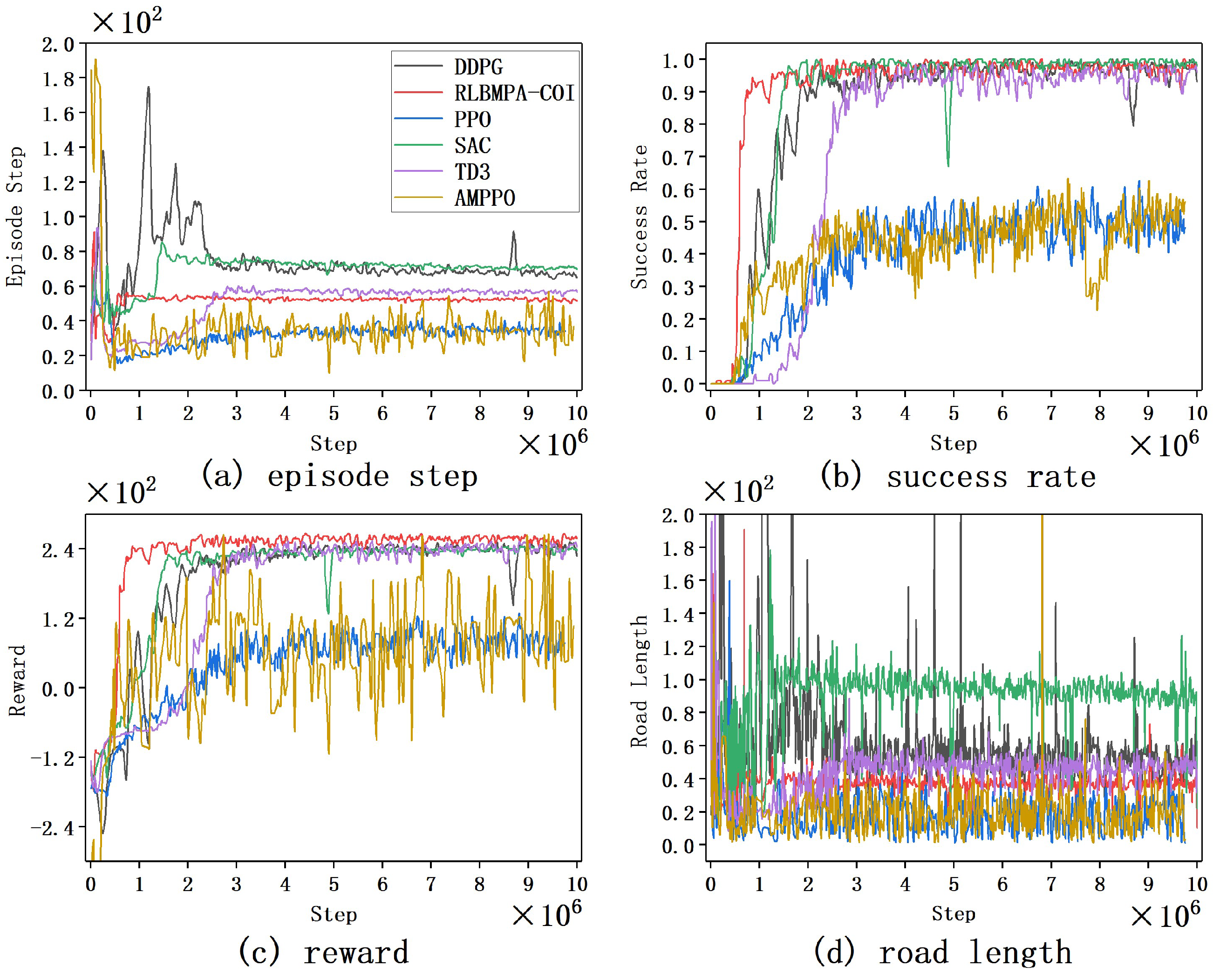
The entire algorithmic training process is shown in Figure 6. Figure 6a shows the average number of steps taken by each algorithm in each episode, Figure 6b shows the success rate of each algorithm, Figure 6c shows the average reward value of each algorithm, and Figure 6d shows the cumulative distance traveled by each algorithm.
At the start of the training process, the AUV selects actions at random to explore its environment. The number of steps taken in each episode is determined by whether the AUV comes into contact with any boundaries or obstacles. Occasional successes result in higher reward values and these experiences are stored in the experience replay pool. As the algorithm converges, the AUV discovers a stable and optimal solution for its path.
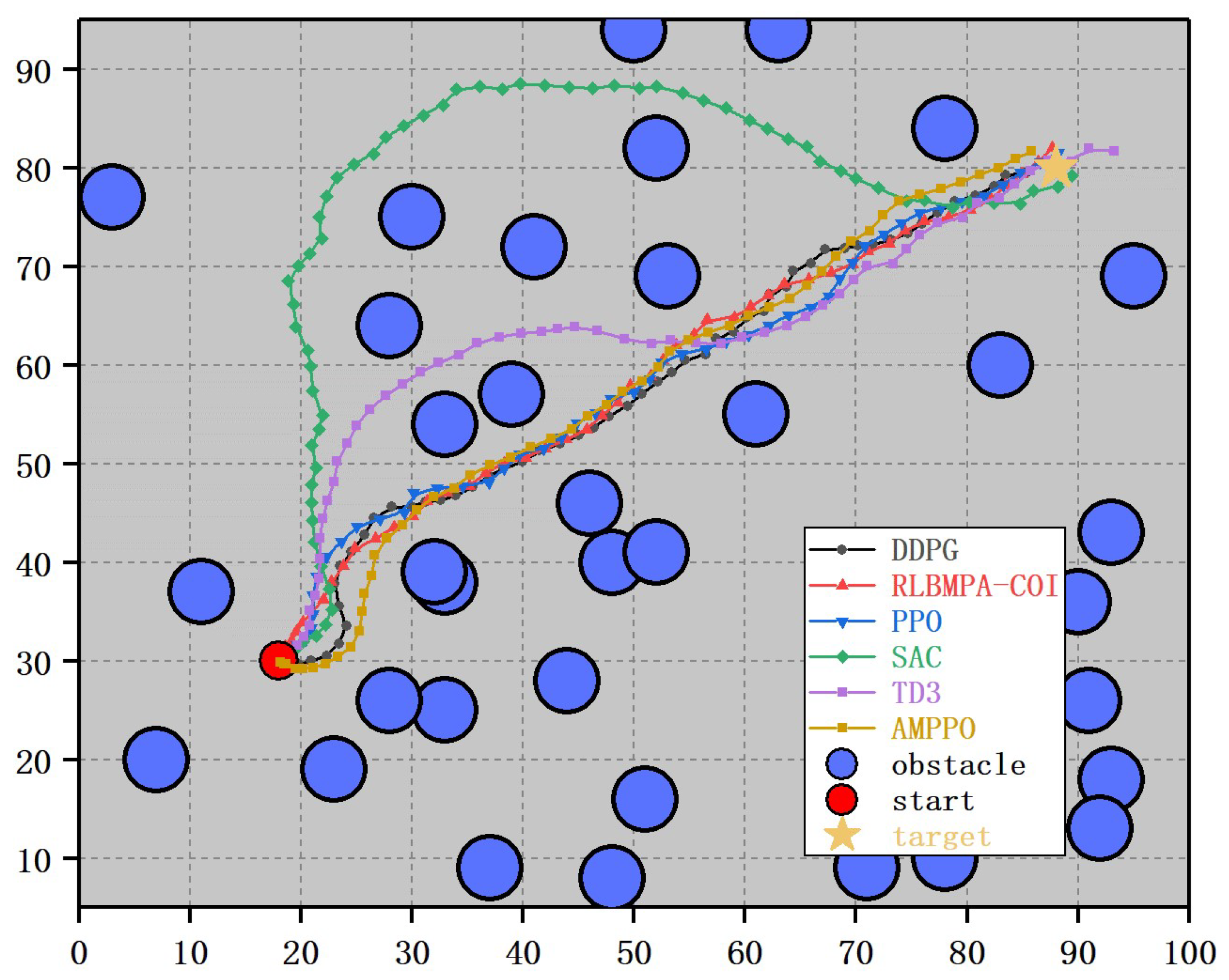
As illustrated in Figure 7, the RLBMPA-COI algorithm converges more quickly due to the action entropy and the reduction in system overestimation errors caused by ocean currents. DDPG and TD3, deterministic policy gradient algorithms, converge to suboptimal solutions when influenced by time-varying ocean currents.

4.2.2. Multi-Objective Path Planning Task

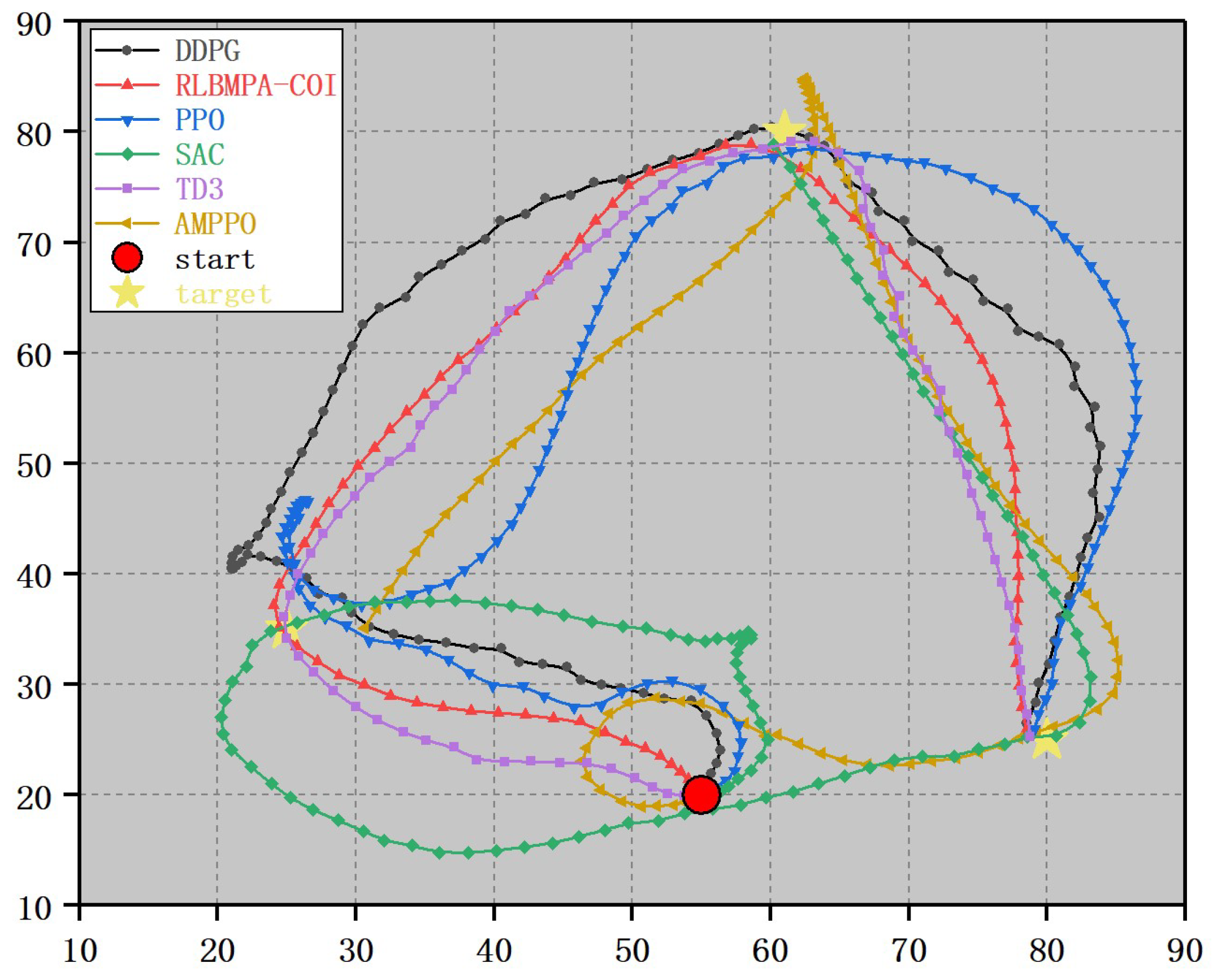
We designed a multi-objective path planning task in which the AUV must navigate around obstacles and reach multiple targets in sequence while being affected by real-time changing ocean currents. The specific goal comprises two fixed targets and one moving target. As illustrated in Figure 8, during each round of training, the AUV is randomly initialized within region 1.
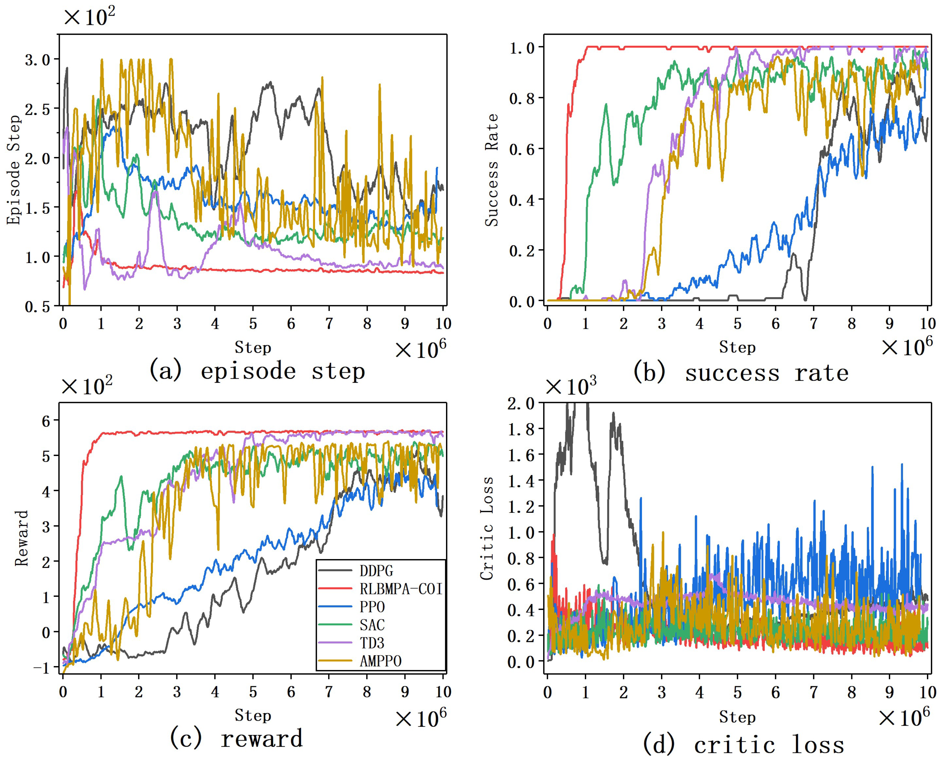
The training process of the algorithm in this environment is shown in Figure 9. The RLBMPA-COI algorithm suppresses the influence of system overestimation errors and takes more accurate actions by incorporating environmental information. Therefore, the algorithm converges faster and maintains a high path planning success rate under the interference of ocean currents, reflecting the strong adaptability of the RLBMPA-COI algorithm. The actual motion paths taken by each algorithm during multi-objective path planning is shown in Figure 10. The RLBMPA-COI algorithm creates a smoother path. When approaching a moving target, its strong robustness enables it to accurately reach the target position, reducing the number of required steps and the cumulative distance.
As shown in Table 1, the initial position and target point position of the AUV are adjusted to test the path planning ability of the algorithm.

4.2.3. Ocean Current Strength Robustness Experiment

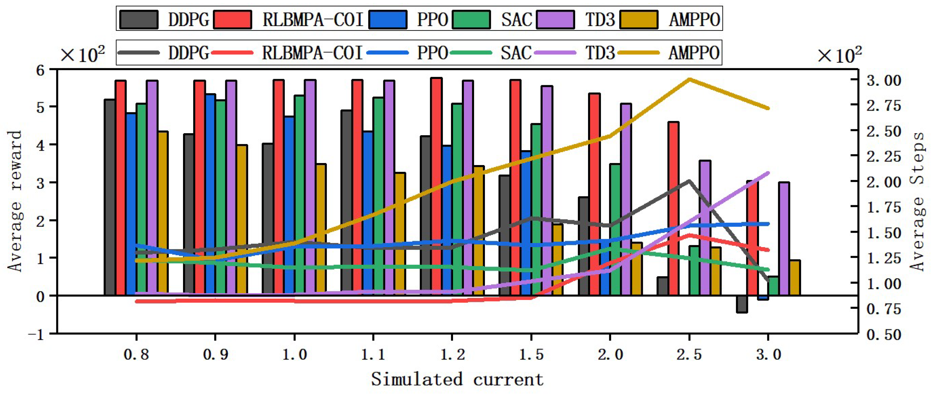
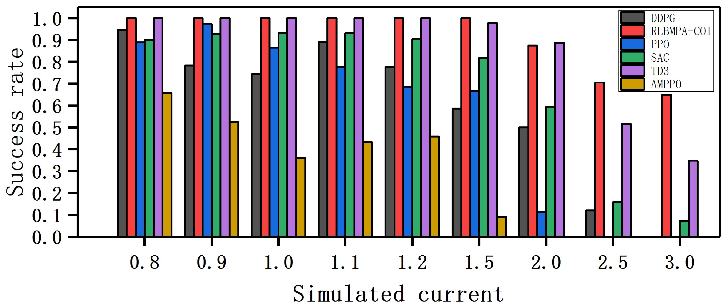
Ocean current intensities are affected by various factors. This study performs a comparative experiment concerning ocean current intensity to evaluate the impacts of different ocean current intensities on path planning algorithms. Specifically, based on multi-objective path planning tasks, all algorithms are trained in actual ocean current environments and tested for robustness under different ocean current intensities by scaling the overall ocean current intensity. Each algorithm is tested for 5000 steps under different current intensities and the average number of steps, average reward and success rate are recorded. The experimental results are shown in Figure 11 and Figure 12.
As the ocean current intensity increases, the average reward and success rate of each algorithm decreased to varying degrees. Among them, only the RLBMPA-COI and TD3 algorithms are able to maintain relative stability under the influence of strong ocean currents. The RLBMPA-COI algorithm had stronger adaptability to ocean current components and can take precise actions with high robustness.

4.2.4. Ocean Current Adaptation Experiment

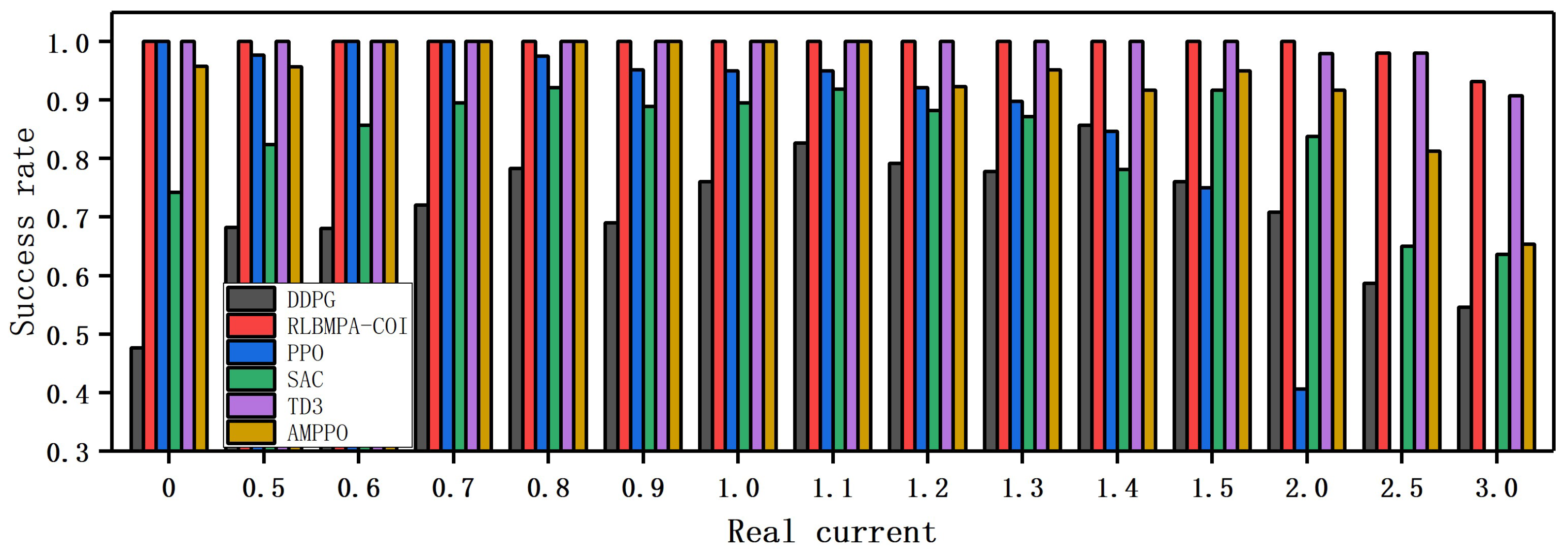
Extreme weather conditions can change the movement patterns of ocean currents, affecting the updating of state transition functions and yielding new data outside the sample distribution range of the training environment. This poses a great challenge to AUV motion planning algorithms based on reinforcement learning. To address this issue, we designed an ocean current adaptability experiment. Specifically, all algorithms are trained in a real ocean current environment and tested in an environment simulated by an ocean current function [36] to test the robustness and adaptability of the algorithm in an out-of-distribution environment. Firstly, we calculated the extreme and average values of real ocean current data. Furthermore, after adjusting the parameters in Equation (4), we fit the simulation to the real ocean current data in extreme and average values. As shown in Table 2:
The experimental results, as illustrated in Figure 13 and Figure 14, reveal that in an out-of-distribution ocean current environment, the DDPG, PPO, and AMPPO algorithms were unable to complete the path planning task. In contrast, the RLBMPA-COI algorithm maintained a high success rate, demonstrating its exceptional adaptability to its environment.

4.3. Trajectory-Tracking Task

In a trajectory-tracking task, an AUV must move along a predetermined path, aligning its motion trajectory with the predetermined path as closely as possible to minimize dynamic tracking errors. Since AUV trajectory-tracking tasks implemented in still water do not take environmental factors into account and the experimental backgrounds are overly idealized, this study focuses on trajectory-tracking tasks under the influence of time-varying ocean currents.

Curve Trajectory-Tracking Task

This task uses a cosine curve as the target trajectory and sets obstacles in the target trajectory path. As shown in Figure 15, the AUV needs to align its own motion trajectory with the target trajectory as well as possibly reduce the induced dynamic tracking error.
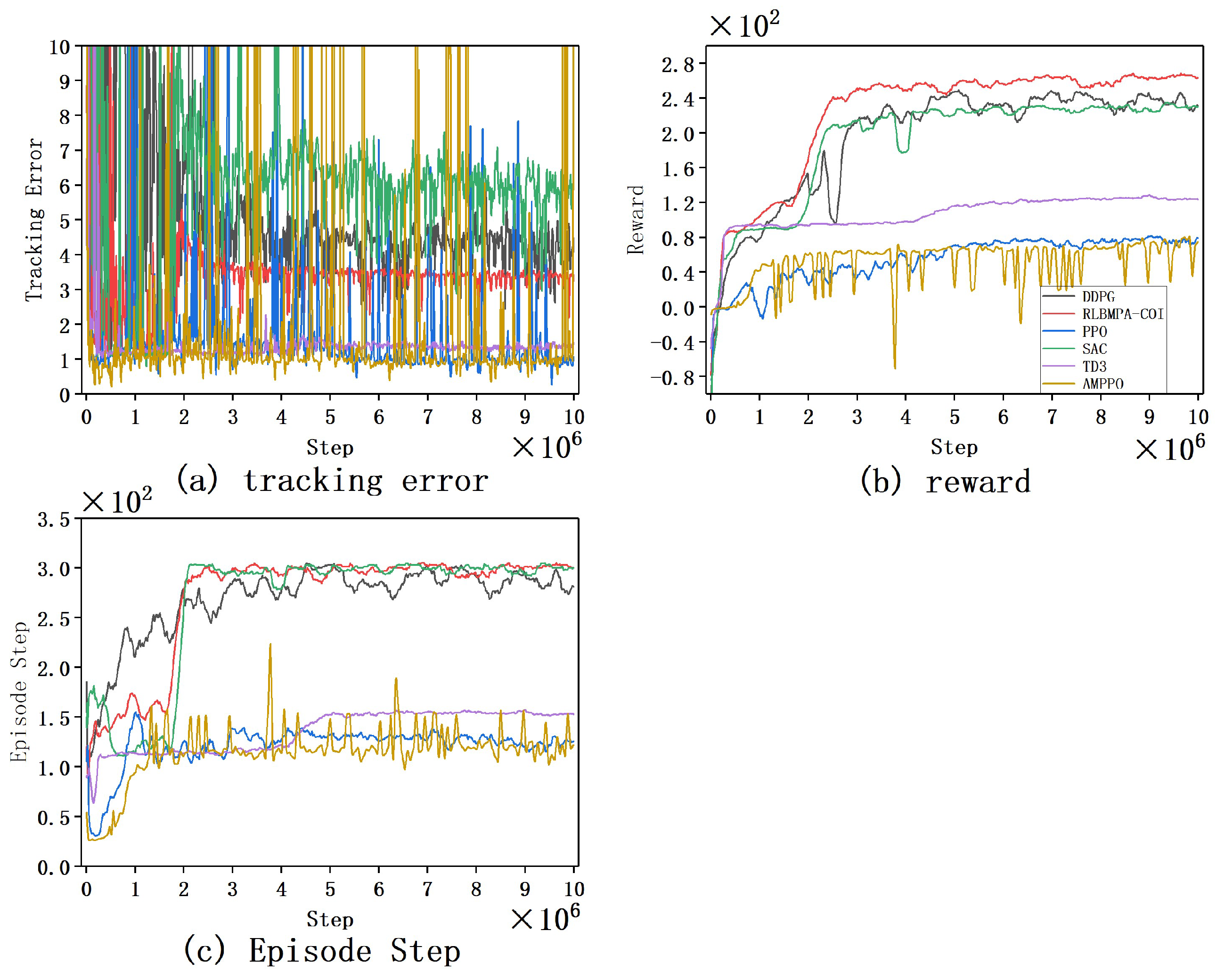
During the training process of the algorithm, obstacles may be present in the target path, preventing the AUV from moving in the direction of the optimal reward. This requires the algorithm to be capable of sacrificing short-term gains for long-term returns. A changing ocean current can interfere with the recording of the AUV’s motion state, causing errors in the algorithm’s estimation of the AUV’s action value. This can result in an overestimation of the state-action value and ultimately lead to a mismatch between the estimated and actual situations, causing the algorithm to become shortsighted or even incorrect. The training process is illustrated in Figure 16.
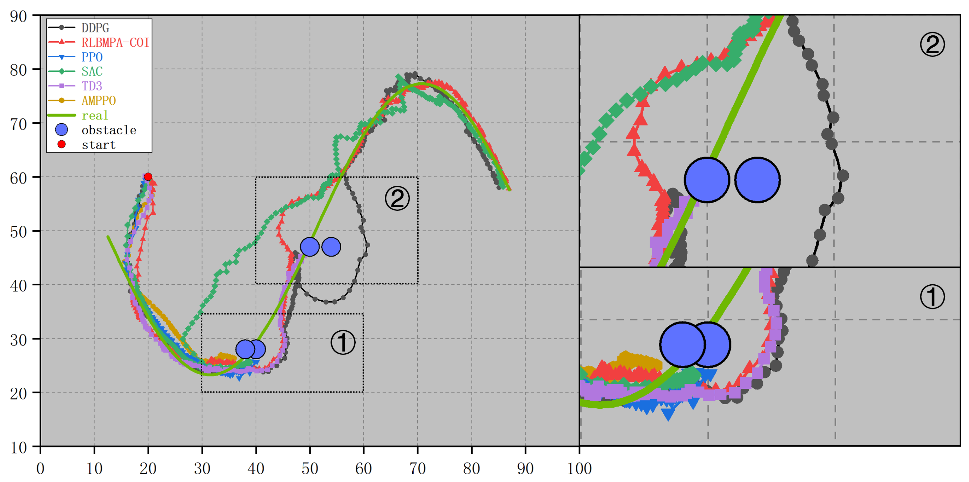
As illustrated in Figure 17, due to the interference of obstacles and ocean currents, the PPO, TD3, and AMPPO algorithms obtain the incorrect estimation of the motion value during training and become trapped in local optima. This is reflected in AUV’s inability to navigate around obstacles during the trajectory-tracking process. In contrast, the RLBMPA-COI, DDPG, and SAC algorithms were able to complete the AUV trajectory-tracking task. Compared to the other algorithms, the RLBMPA-COI algorithm is better able to adjust the AUV’s motion state to bring its trajectory closer to the target trajectory, resulting in smaller tracking errors. Additionally, when the tracking errors and ocean currents are accounted for in the reward function, the average return value yielding the AUV trajectory-tracking algorithm based on the RLBMPA-COI algorithm is the highest.

5. Conclusions

In this work, we introduce the RLBMPA-COI algorithm, a multitask motion planning approach for an AUV operating in ocean environments. The algorithm incorporates realtime ocean current data into an environmental model to balance realism and complexity, providing robust support for multitask environments and addressing the limitations exhibited by existing methods. We combine an AUV motion model with environmental data to accurately represent the environmental features and design a reinforcement learning environment for multiple AUV motion planning tasks. The RLBMPA-COI algorithm builds on the SAC algorithm to capture and integrate variations in ocean currents, reducing the overestimation caused by current motion and significantly enhancing the stability and practicality of the algorithm. We evaluate the performance of our algorithm across multiple task environments and demonstrate that the RLBMPA-COI algorithm outperforms other methods in target exploration tasks conducted in scenarios with dense obstacles and multipoint targets. The RLBMPA-COI algorithm also exhibits excellent stability in scenarios with the changing ocean current strength and simulated ocean currents. Furthermore, the RLBMPA-COI algorithm maintains its effective trajectory-tracking effect in complex environments.

Author Contributions

Conceptualization, Y.L.; methodology, Y.L. and X.H.; software, X.H.; validation, Y.L., X.H. and P.J.; formal analysis, Y.L.; investigation, Y.L.; resources, Y.L.; data curation, X.H.; writing—original draft preparation, X.H.; writing—review and editing, Y.L. and X.H.; visualization, Y.L. and X.H.; supervision, Y.L., Z.L. and Y.S.; project administration, Y.L.; funding acquisition, Y.L. All authors have read and agreed to the published version of the manuscript.

Funding

This work was funded by the National Natural Science Foundation of China (grant number 61861014); the Doctor Start-Up Fund (grant number BS2021025).

Data Availability Statement

The data that support the findings of this study are available from the corresponding author upon reasonable request.

Conflicts of Interest

The authors declare no conflict of interest.

Appendix A

Table A1. Notations.
NameDescription
η AUV state vector
x , y , z Surge, sway and heave in the global coordinate system
σ , β , χ Roll, pitch and yaw in the global coordinate system
v Velocity vector of the AUV
u , v , w Velocity components in the body coordinate system
g , h , j Angular velocity components in the body coordinate system
tMoment of AUV motion
C u r max Maximum change in ocean current
C u r x , C u r y The strength of the ocean current components in the global coordinate system
C u r ( x t , y t ) The vector of the ocean current at time t
k 1 , k 2 , k 3 , λ Environmental influence parameters
k 4 , k 5 Stochastic influence parameters
D i s o Distance between the AUV and the obstacle
D i s t Distance between the AUV and the target
D i s l Relative distance between the obstacle and the nearest target
S w Obstacle warning range
S c Obstacle collision range
S t a r Target perceived distance
δ a u v The range of angles output by the movement of the AUV
PThe position of the AUV
P i g o a l The position of the i-th target point
k i g o a l The completion status of the i-th target point
θ 1 , θ 2 State value network parameters
θ 1 , θ 2 Target state value network parameters
ϕ Policy network parameters
α t Action entropy value weight
ε σ , ε β Systematic error caused by ocean currents in the longitudinal and transverse directions
B σ , b , Δ σ The amplitude, frequency and phase of the longitudinal ocean current
C β , c , Δ β The amplitude, frequency and phase of the transverse ocean current
γ x , γ y The weights of ocean currents for algorithm updates
Table A2. Algorithm training parameters.
ParameterValue
Ocean current weight coefficient γ c u r 0.4
Step weight coefficient λ s t e p 10 e 4
The completion status of the i-th target point k i g o a l 1 or 10 e 4
Obstacle warning range S w 0.2
Obstacle collision range S c 0.05
Target perceived distance S t a r 0.05
AUV turning angle range δ a u v [ 0.25 π , 0.25 π ]
Learning rate 3 e 4
Replay buffer D capacity B r 10 e 6
Current weight queue u e c u r capacity B q u e 10 e 4
Total training steps T 10 e 6
Maximum training steps per episode T e 300
Gradient update frequency f g 1
Update weight of the policy network λ ϕ 0.005
Discount factor γ 0.99
Table A3. Algorithm hyperparameter statistics.
Algorithm NameDDPGRLBMPA-COIPPOSACTD3AMPPO
Total training steps T 10 e 6 10 e 6 10 e 6 10 e 6 10 e 6 10 e 6
Learning rate 10 e 3 3 e 4 3 e 4 3 e 4 10 e 3 3 e 4
Replay buffer D capacity B r 10 e 6 10 e 6 None 10 e 6 10 e 6 None
Discount factor γ 0.990.990.990.990.990.99
Update weight of the policy network λ ϕ 0.0050.005None0.0050.005None
Current weight queue u e c u r capacity B q u e None 10 e 4 NoneNoneNoneNone
Target policy noiseNoneNoneNoneNone0.2None
Number of processes111112
Generalized advantage estimation (GAE)NoneNone0.95NoneNone0.95

References

  1. Zhao, W.; Zhao, H.; Liu, G.; Zhang, G. ANFIS-EKF-Based Single-Beacon Localization Algorithm for AUV. Remote Sens. 2022, 14, 5281. [Google Scholar] [CrossRef]
  2. Cai, C.; Chen, J.; Yan, Q.; Liu, F. A Multi-Robot Coverage Path Planning Method for Maritime Search and Rescue Using Multiple AUVs. Remote Sens. 2022, 15, 93. [Google Scholar] [CrossRef]
  3. Sun, Y.; Song, H.; Jara, A.J.; Bie, R. Internet of things and big data analytics for smart and connected communities. IEEE Access 2016, 4, 766–773. [Google Scholar] [CrossRef]
  4. Yu, H.; Meier, K.; Argyle, M.; Beard, R.W. Cooperative path planning for target tracking in urban environments using unmanned air and ground vehicles. IEEE/ASME Trans. Mechatronics 2014, 20, 541–552. [Google Scholar] [CrossRef]
  5. Takahashi, O.; Schilling, R.J. Motion planning in a plane using generalized Voronoi diagrams. IEEE Trans. Robot. Autom. 1989, 5, 143–150. [Google Scholar] [CrossRef]
  6. Mueller, T.G.; Pusuluri, N.B.; Mathias, K.K.; Cornelius, P.L.; Barnhisel, R.I.; Shearer, S.A. Map quality for ordinary kriging and inverse distance weighted interpolation. Soil Sci. Soc. Am. J. 2004, 68, 2042–2047. [Google Scholar] [CrossRef]
  7. Wang, G.; Wei, F.; Jiang, Y.; Zhao, M.; Wang, K.; Qi, H. A Multi-AUV Maritime Target Search Method for Moving and Invisible Objects Based on Multi-Agent Deep Reinforcement Learning. Sensors 2022, 22, 8562. [Google Scholar] [CrossRef]
  8. Yokota, Y.; Matsuda, T. Underwater Communication Using UAVs to Realize High-Speed AUV Deployment. Remote Sens. 2021, 13, 4173. [Google Scholar] [CrossRef]
  9. Sedighi, S.; Nguyen, D.V.; Kuhnert, K.D. Guided hybrid A-star path planning algorithm for valet parking applications. In Proceedings of the 2019 5th International Conference on Control, Automation and Robotics (ICCAR), Beijing, China, 19–22 April 2019; pp. 570–575. [Google Scholar]
  10. Zhu, J.; Zhao, S.; Zhao, R. Path planning for autonomous underwater vehicle based on artificial potential field and modified RRT. In Proceedings of the 2021 International Conference on Computer, Control and Robotics (ICCCR), Shanghai, China, 8–10 January 2021; pp. 21–25. [Google Scholar]
  11. Chen, L.; Shan, Y.; Tian, W.; Li, B.; Cao, D. A fast and efficient double-tree RRT*-like sampling-based planner applying on mobile robotic systems. IEEE/ASME Trans. Mechatron. 2018, 23, 2568–2578. [Google Scholar] [CrossRef]
  12. Nayeem, G.M.; Fan, M.; Akhter, Y. A time-varying adaptive inertia weight based modified PSO algorithm for UAV path planning. In Proceedings of the 2021 2nd International Conference on Robotics, Electrical and Signal Processing Techniques (ICREST), Dhaka, Bangladesh, 5–7 January 2021; pp. 573–576. [Google Scholar]
  13. Yang, H.; Qi, J.; Miao, Y.; Sun, H.; Li, J. A new robot navigation algorithm based on a double-layer ant algorithm and trajectory optimization. IEEE Trans. Ind. Electron. 2018, 66, 8557–8566. [Google Scholar] [CrossRef] [Green Version]
  14. Roberge, V.; Tarbouchi, M.; Labonté, G. Comparison of parallel genetic algorithm and particle swarm optimization for real-time UAV path planning. IEEE Trans. Ind. Inform. 2012, 9, 132–141. [Google Scholar] [CrossRef]
  15. Shen, C.; Buckham, B.; Shi, Y. Modified C/GMRES algorithm for fast nonlinear model predictive tracking control of AUVs. IEEE Trans. Control. Syst. Technol. 2016, 25, 1896–1904. [Google Scholar] [CrossRef]
  16. Li, Z.; Deng, J.; Lu, R.; Xu, Y.; Bai, J.; Su, C.Y. Trajectory-tracking control of mobile robot systems incorporating neural-dynamic optimized model predictive approach. IEEE Trans. Syst. Man Cybern. Syst. 2015, 46, 740–749. [Google Scholar] [CrossRef]
  17. Ang, K.H.; Chong, G.; Li, Y. PID control system analysis, design, and technology. IEEE Trans. Control. Syst. Technol. 2005, 13, 559–576. [Google Scholar]
  18. Joseph, S.B.; Dada, E.G.; Abidemi, A.; Oyewola, D.O.; Khammas, B.M. Metaheuristic algorithms for PID controller parameters tuning: Review, approaches and open problems. Heliyon 2022, 8, e09399. [Google Scholar] [CrossRef]
  19. Konar, A.; Chakraborty, I.G.; Singh, S.J.; Jain, L.C.; Nagar, A.K. A deterministic improved Q-learning for path planning of a mobile robot. IEEE Trans. Syst. Man Cybern. Syst. 2013, 43, 1141–1153. [Google Scholar] [CrossRef] [Green Version]
  20. Du, J.; Jiang, C.; Wang, J.; Ren, Y.; Debbah, M. Machine learning for 6G wireless networks: Carrying forward enhanced bandwidth, massive access, and ultrareliable/low-latency service. IEEE Veh. Technol. Mag. 2020, 15, 122–134. [Google Scholar] [CrossRef]
  21. Wang, J.; Wu, Z.; Yan, S.; Tan, M.; Yu, J. Real-time path planning and following of a gliding robotic dolphin within a hierarchical framework. IEEE Trans. Veh. Technol. 2021, 70, 3243–3255. [Google Scholar] [CrossRef]
  22. Han, G.; Zhou, Z.; Zhang, T.; Wang, H.; Liu, L.; Peng, Y.; Guizani, M. Ant-colony-based complete-coverage path-planning algorithm for underwater gliders in ocean areas with thermoclines. IEEE Trans. Veh. Technol. 2020, 69, 8959–8971. [Google Scholar] [CrossRef]
  23. Huang, B.Q.; Cao, G.Y.; Guo, M. Reinforcement learning neural network to the problem of autonomous mobile robot obstacle avoidance. In Proceedings of the 2005 International Conference on Machine Learning and Cybernetics, Guangzhou, China, 18–21 August 2005; Volume 1, pp. 85–89. [Google Scholar]
  24. Mnih, V.; Kavukcuoglu, K.; Silver, D.; Rusu, A.A.; Veness, J.; Bellemare, M.G.; Hassabis, D. Human-level control through deep reinforcement learning. Nature 2015, 518, 529–533. [Google Scholar] [CrossRef]
  25. Chu, Z.; Wang, F.; Lei, T.; Luo, C. Path planning based on deep reinforcement learning for autonomous underwater vehicles under ocean current disturbance. IEEE Trans. Intell. Veh. 2022, 8, 108–120. [Google Scholar] [CrossRef]
  26. Zhang, C.; Cheng, P.; Du, B.; Dong, B.; Zhang, W. AUV path tracking with real-time obstacle avoidance via reinforcement learning under adaptive constraints. Ocean Eng. 2022, 256, 111453. [Google Scholar]
  27. Hou, Y.; Liu, L.; Wei, Q.; Xu, X.; Chen, C. A novel DDPG method with prioritized experience replay. In Proceedings of the 2017 IEEE International Conference on Systems, Man, and Cybernetics (SMC), Banff, AB, Canada, 5–8 October 2017; pp. 316–321. [Google Scholar]
  28. Du, J.; Zhou, D.; Wang, W.; Arai, S. Reference Model-Based Deterministic Policy for Pitch and Depth Control of Autonomous Underwater Vehicle. J. Mar. Sci. Eng. 2023, 11, 588. [Google Scholar]
  29. Hadi, B.; Khosravi, A.; Sarhadi, P. Deep reinforcement learning for adaptive path planning and control of an autonomous underwater vehicle. Appl. Ocean Res. 2023, 129, 103326. [Google Scholar]
  30. Fujimoto, S.; Hoof, H.; Meger, D. Addressing function approximation error in actor-critic methods. In Proceedings of the 35th International Conference on Machine Learning, Stockholm, Sweden, 10–15 July 2018; pp. 1587–1596. [Google Scholar]
  31. Xu, J.; Huang, F.; Wu, D.; Cui, Y.; Yan, Z.; Du, X. A learning method for AUV collision avoidance through deep reinforcement learning. Ocean Eng. 2022, 260, 112038. [Google Scholar]
  32. Huang, F.; Xu, J.; Yin, L.; Wu, D.; Cui, Y.; Yan, Z.; Chen, T. A general motion control architecture for an autonomous underwater vehicle with actuator faults and unknown disturbances through deep reinforcement learning. Ocean Eng. 2022, 263, 112424. [Google Scholar]
  33. Haarnoja, T.; Zhou, A.; Abbeel, P.; Levine, S. Soft actor-critic: Off-policy maximum entropy deep reinforcement learning with a stochastic actor. In Proceedings of the 35th International Conference on Machine Learning, Stockholm, Sweden, 10–15 July 2018; pp. 1861–1870. [Google Scholar]
  34. He, Z.; Dong, L.; Sun, C.; Wang, J. Asynchronous multithreading reinforcement-learning-based path planning and tracking for unmanned underwater vehicle. IEEE Trans. Syst. Man Cybern. Syst. 2021, 52, 2757–2769. [Google Scholar]
  35. Wang, Y.; He, H.; Tan, X. Truly proximal policy optimization. In Proceedings of the Uncertainty in Artificial Intelligence, Tel Aviv, Israel, 22–25 July 2019; pp. 113–122. [Google Scholar]
  36. Jaffe, J.; Schurgers, C. Sensor networks of freely drifting autonomous underwater explorers. In Proceedings of the 1st International Workshop on Underwater Networks, Los Angeles, CA, USA, 25 September 2006; pp. 93–96. [Google Scholar]
  37. Xi, M.; Yang, J.; Wen, J.; Liu, H.; Li, Y.; Song, H.H. Comprehensive ocean information-enabled AUV path planning via reinforcement learning. IEEE Internet Things J. 2022, 9, 17440–17451. [Google Scholar]
  38. National Marine Science and Technology Center. Available online: http://mds.nmdis.org.cn/ (accessed on 1 May 2022).
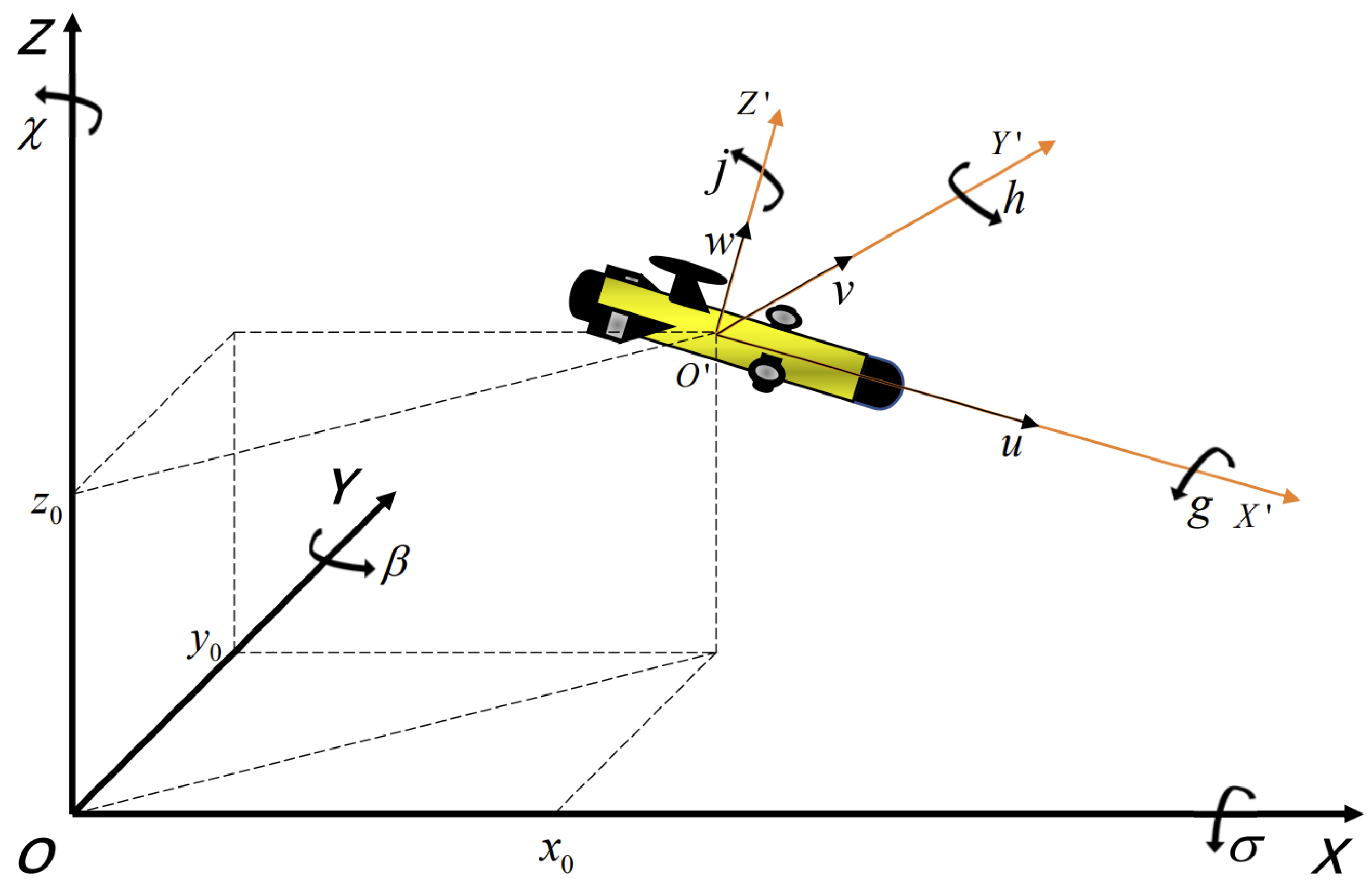
Figure 1. AUV motion model.
Remotesensing 15 03077 g001
Figure 2. Changes in the ocean current model at each time step in reinforcement learning.
Remotesensing 15 03077 g002
Figure 3. Ocean current changes.
Remotesensing 15 03077 g003
Figure 4. Algorithmic structure diagram.
Remotesensing 15 03077 g004
Figure 5. Path planning tasks with complex obstacles.
Remotesensing 15 03077 g005
Figure 6. Training process in a complex obstacle environment.
Remotesensing 15 03077 g006
Figure 7. Path planning results for a complex obstacle environment.
Remotesensing 15 03077 g007
Figure 8. Multi-objective path planning effect.
Remotesensing 15 03077 g008
Figure 9. Multi-objective path planning training process.
Remotesensing 15 03077 g009
Figure 10. Multi-objective path planning training process.
Remotesensing 15 03077 g010
Figure 11. Changes in the number of steps and the reward values with current intensity changes.
Remotesensing 15 03077 g011
Figure 12. Changes in the success rate when the current intensity changes.
Remotesensing 15 03077 g012
Figure 13. Changes in the next steps and reward value with the functional current model.
Remotesensing 15 03077 g013
Figure 14. Changes in the success rate with the functional current model.
Remotesensing 15 03077 g014
Figure 15. Trajectory-tracking task.
Remotesensing 15 03077 g015
Figure 16. Training process in a complex obstacles environment.
Remotesensing 15 03077 g016
Figure 17. Trajectory-tracking results.
Remotesensing 15 03077 g017
Table 1. Path planning location change table.
PathStart PointTerminal PointAMPPOSACRLBMPA-COI
StepRewardStepRewardStepReward
1(55,20)(25,35), (60,80), (80,25)107.25535.4122.75548.4584.4567.26
2(65,10)(25,35), (60,80), (80,25)118.7527.76106553.2585561.58
3(55,20)(25,35), (60,65), (80,35)116.35533.79107.32563.3482.25573.46
4(65,10)(25,35), (60,65), (80,35)118.5529.83109.25556.5987.65563.05
Table 2. Ocean current model parameters.
ParameterValue
Maximum speed of ocean currents C u r max 1.892
Environmental influence parameters of ocean currents λ 3.018
Environmental influence parameters of ocean currents k 1 , k 2 , k 3 3.122, 3.023, 3.034
Stochastic influence parameters of ocean currents k 4 , k 5 1.015, 0.987
Disclaimer/Publisher’s Note: The statements, opinions and data contained in all publications are solely those of the individual author(s) and contributor(s) and not of MDPI and/or the editor(s). MDPI and/or the editor(s) disclaim responsibility for any injury to people or property resulting from any ideas, methods, instructions or products referred to in the content.