Improve the Accuracy in Numerical Modeling of Suspended Sediment Concentrations in the Hangzhou Bay by Assimilating Remote Sensing Data Utilizing Combined Techniques of Adjoint Data Assimilation and the Penalty Function Method

Abstract

Suspended sediment dynamics play an important role in controlling nearshore and estuarine geomorphology and the associated ecological environments. Modeling the transport of suspended sediment is a complicated and challenging research topic. The goal of this study is to improve the accuracy of modeling the suspended sediment concentrations (SSCs) with newly developed techniques. Based on a three-dimensional suspended cohesive sediment transport model, the transport of suspended sediment and SSCs are simulated by assimilating SSCs retrieved from the Geostationary Ocean Color Imager (GOCI) with the adjoint data assimilation in the Hangzhou Bay, a typical strong tidal estuary along the coast of the East China Sea. To improve the effect of the data assimilation, the penalty function method, in which the reasonable constraints of the estimated model parameters are added to the cost function as penalty terms, will be introduced for the first time into the adjoint data assimilation in the SSCs modeling. In twin experiments, the prescribed spatially varying settling velocity is estimated by assimilating the synthetic SSC observations, and the results show that the penalty function method can further improve the effect of data assimilation and parameter estimation, regardless of synthetic SSC observations being contaminated by random artificial errors. In practical experiments, the spatially varying settling velocity is firstly estimated by assimilating the actual GOCI-retrieved SSCs. The results demonstrate that the simulated results can be improved by the adjoint data assimilation, and the penalty function method can additionally reduce the mean absolute error (MAE) between the independent check observations and the corresponding simulated SSCs from 1.44 × 10⁻¹ kg/m³ to 1.30 × 10⁻¹ kg/m³. To pursue greater simulation accuracy, the spatially varying settling velocity, resuspension rate, critical shear stress and initial conditions are simultaneously estimated by assimilating the actual GOCI-retrieved SSCs to simulate the SSCs in the Hangzhou Bay. When the adjoint data assimilation and the penalty function method are simultaneously used, the MAE between the independent check observations and the corresponding simulated SSCs is just 9.90 × 10⁻² kg/m³, which is substantially less than that when only the settling velocity is estimated. The MAE is also considerably less than that when the four model parameters are estimated to be without using the penalty function method. This study indicates that the adjoint data assimilation can effectively improve the SSC simulation accuracy, and the penalty function method can limit the variation range of the estimated model parameters to further improve the effect of data assimilation and parameter estimation.

1. Introduction

The spatial and temporal distribution of suspended sediment concentrations (SSCs) in nearshore and estuarine waters are usually complex due to river input, tidal effects and local sediment resuspension [1]. Suspended sediment is the main carrier of pollutants and can also affect the ecological environment by reducing the transparency of the sea water [2,3]. In addition, the transport of suspended sediment affects the geomorphological features and riverbed evolution of the nearshore and estuarine area [4]. The Hangzhou Bay is a typical strong tidal estuary in China, with significant characteristics such as large tidal range, rapid tidal currents, high sediment content in the water column and complex suspended sediment transport processes [5,6]. It is of great scientific significance and practical value to improve accuracy of modeling the temporal and spatial distribution and transport of suspended sediment in the Hangzhou Bay.

For the study of spatial and temporal distribution and transport of suspended sediment, field observations with various techniques, including optical, acoustic and traditional water collector sampling methods, are commonly used. The SSCs measured by the traditional water collector sampling method have high accuracy, but the spatial and temporal resolutions are low due to its time-consuming and labor-intensive features [7]. Hamilton et al. [8] summarized and compared the acoustic and optical observation methods, and they pointed out that the spatial and temporal resolution of SSCs obtained by the acoustic and optical observation methods are higher than that of the water collector sampling method. When the SSCs are extraordinarily high, however, the signal will be attenuated, leading to large errors in the observations. In addition, studies on the distribution and transport of surface-suspended sediment in estuaries, nearshore and other shallow sea areas using satellite remote sensing data have gradually increased in recent years [9,10,11,12,13]. It is worth noting that the remote sensing methods can usually only obtain the distribution of suspended sediment at the sea surface, and the retrieved SSCs will be missing, to a certain extent, when cloud cover exists [14,15]. Mathematical modeling of suspended sediment transport has gradually become an important technique in nearshore science [16,17,18,19,20]. The mathematical model of suspended sediment transport has evolved from the original one-dimensional to multi-dimensional, and has been associated with considerable improvement in SSC simulation [21]. Therefore, numerical simulation is an effective method to quantify the dynamics of suspended sediment transport [22,23], with the characteristics of low cost, strong portability and predictability. The numerical models can effectively obtain the temporal and spatial (horizontal and vertical) distribution of SSCs, which provide compensation for the low spatial resolution of in situ observations, and also offer alternative data for the no vertical structure of SSC derived from remote sensing methods [24].

However, an important feature of suspended sediment transport models is that they are highly empirical, and the model parameters need to be fully calibrated in different application cases [20]. How to effectively estimate the model parameters from the results of laboratory experiments or field observations has become an important scientific question directly related to the predictability of suspended sediment transport models [25]. In traditional numerical simulation studies of suspended sediment transport, the model parameters are artificially adjusted to reduce the errors between the simulated and the observed results. Apparently, this approach cannot achieve the simultaneous optimal estimation of multiple model parameters and fails to provide a reasonable estimation of the spatially or temporally varying model parameters. Fringer et al. [26] pointed out that the data assimilation methods could quantitatively estimate unknown or difficult-to-measure model parameters by assimilating observed data. At the same time, data assimilation can combine the advantages of observational data and mathematical models to minimize the difference between the simulation results and their true values [27,28]. Many studies have simulated SSCs using the data assimilation [25,29,30,31,32,33]. Adjoint data assimilation is an effective method to improve accuracy in the simulation of near-shore SSCs by optimizing model parameters [33]. Wang et al. [21,33] has developed a three-dimensional suspended cohesive sediment transport model to simulate the SSCs in the Hangzhou Bay using adjoint data assimilation. The independent point scheme and Tikhonov regularization method were combined and used into the adjoint data assimilation to further improve the simulation accuracy [34].

In fact, it should be noted that the model parameters have a certain variation range, which needs to be considered when estimating model parameters using the adjoint data assimilation [33]. The penalty function method is an effective method to solve such constrained optimization problems [35,36] and has been applied in the fields of atmosphere and mechanical engineering [37,38], but the penalty function method has not been systematically investigated in the field of SSC modeling. In this paper, based on the existing model by Wang et al. [33], the penalty function method will be utilized for the first time in the three-dimensional suspended cohesive sediment transport model to ensure that the model parameters are always kept within a reasonable range during the processes of parameter estimation. In addition, the transport of suspended sediment and SSCs in the Hangzhou Bay are simulated by assimilating the SSCs retrieved from the Geostationary Ocean Color Imager (GOCI) with the adjoint data assimilation and the penalty function method. The structure of the paper is as follows: Section 2 presents the three-dimensional suspended cohesive sediment transport model with adjoint data assimilation, the penalty function method and the GOCI-retrieved SSCs. The twin and practical experiments are designed and performed in Section 3 and Section 4, respectively. The conclusion and discussion are shown in Section 5.

2. Models and Data

2.1. Models

2.1.1. The Suspended Cohesive Sediment Transport Model

The governing equation of the three-dimensional suspended cohesive sediment transport model is as follows [33]:

$$\frac{\partial C}{\partial t}+u\frac{\partial C}{\partial x}+v\frac{\partial C}{\partial y}+w\frac{\partial C}{H\partial \sigma }=\frac{\partial }{\partial x}\left(K_H\frac{\partial C}{\partial x}\right)+\frac{\partial }{\partial y}\left(K_H\frac{\partial C}{\partial y}\right)+\frac{\partial }{H\partial \sigma }\left(K_V\frac{\partial C}{H\partial \sigma }\right){+w}_s\frac{\partial C}{H\partial \sigma })$$

(1)

where C is SSCs; t is the time; x and y are horizontal coordinates; $\sigma$ is the vertical coordinate (in the range 0 to 1, 0 is the bottom, 1 is the sea surface); H is the total water depth including the static water depth and the sea surface elevation; u, v and w are the flow velocities in the x, y and $\sigma$ directions, respectively; $K_H$ and $K_V$ are the horizontal and vertical diffusion coefficients, respectively; $w_s$ is the settling velocity of the suspended sediment.

The inflow open boundary condition is:

$${C=C}_{\mathit{obc}}$$

(2)

where $C_{\mathit{obc}}$ is the SSCs at the inflow opening boundary (river boundary).

The ocean boundary condition is:

$$\frac{\partial C}{\partial \overrightarrow{n}}=0$$

(3)

where $\overrightarrow{n}$ is the outer normal vector of the boundary.

The land boundary condition is:

$$K_H\frac{\partial C}{\partial \overrightarrow{n}}=0$$

(4)

The sea surface boundary condition is:

$$-w_s·C-\frac{K_V}{H}\frac{\partial C}{\partial \sigma }=0,\sigma =1$$

(5)

The bottom boundary condition is:

$$-w_s·C-\frac{K_V}{H}\frac{\partial C}{\partial \sigma }=E-D,\sigma =0$$

(6)

where E and D represent the erosion rate and the deposition rate, respectively, and the calculation formulas are [39]:

$$E=\left\{\begin{array}{cc}{M}_0·\frac{{\tau }_b-{\tau }_{\mathit{ce}}}{{\tau }_{\mathit{ce}}},& {\tau }_b{>\tau }_{\mathit{ce}}\\ 0,& {\tau }_b⩽{\tau }_{\mathit{ce}}\end{array}\right.$$

(7)

$$D=\left\{\begin{array}{cc}{w}_s·C_1·\frac{{\tau }_{\mathit{cd}}-{\tau }_b}{{\tau }_{\mathit{cd}}},& {\tau }_b{<\tau }_{\mathit{cd}}\\ 0,& {\tau }_b⩾{\tau }_{\mathit{cd}}\end{array}\right.$$

(8)

where $M_0$ is the resuspension rate; ${\tau }_{\mathit{ce}}$ is the critical shear stress for erosion; ${\tau }_{\mathit{cd}}$ is the critical shear stress for deposition; $C_1$ is the SSCs near the seafloor; and ${\tau }_b$ is the bottom shear stress. The critical shear stresses for erosion and deposition are assumed to be equal in this study and uniformly noted as critical shear stress $\tau$.

In addition, the initial condition is:

$${\left.C\right|}_{t=0}{=C}_0$$

(9)

where $C_0$ is the initial distribution of SSCs.

Detailed information regarding difference scheme and specific solution process of the suspended cohesive sediment transport model can refer to Wang et al. [33].

2.1.2. The Adjoint Model

To construct the discrete adjoint model, the augmented cost function J is defined according to the penalty function method, as follows:

$$J=\frac{1}{2}{\displaystyle \sum }_{i,j,k,n}\left[W_{i,j,k}^n{\left(C_{i,j,k}^n-{\overline{C}}_{i,j,k}^n\right)}^2{+\delta \mu }_{i,j,k}^{n}g\left(p_{i,j,k}^n\right)\right]$$

(10)

where $C_{i,j,k}^n$ and ${\overline{C}}_{i,j,k}^n$ are the simulated and observed SSCs at the nth time step at grid point $(i,j,k)$, respectively; $W_{i,j,k}^n$ is the corresponding element in the weight matrix W. In this paper, it is assumed that the errors between the observed data are uncorrelated and equally weighted, and the weight matrix W satisfies the condition, as follows:

$$\left\{\begin{array}{l}{W}_{i,j,k}^n=1,\mathrm{Observations}\mathrm{are}\mathrm{available}\mathrm{at}(i,j,k,n)\hfill \\ W_{i,j,k}^n=0,\mathrm{No}\mathrm{observation}\mathrm{at}(i,j,k,n)\hfill \end{array}\right.$$

(11)

In addition, the second term in the square brackets of Equation (10) is the penalty term, and the value of $\mathsf{\delta }$ is 1 or 0. When $\mathsf{\delta }$ is equal to 1, it means that the penalty function method is used, and when $\delta$ is equal to 0, the penalty function method is not used. $p_{i,j,k}^n$ is the value of the model parameters at the nth time step at grid point $(i,j,k)$; ${\mu }_{i,j,k}^n$ is the penalty coefficient corresponding to the model parameters; ${g(p}_{i,j,k}^n)$ is the penalty function, and the specific calculation formula is as follows:

$${g(p}_{i,j,k}^n)=\left\{\begin{array}{cc}\frac{1}{2}{\left(p_{i,j,k}^n-p^{\mathit{max}}\right)}^2\hfill & {\mathrm{if}p}_{i,j,k}^n{>p}^{\mathit{max}}\hfill \\ 0& {\mathrm{if}p}^{\mathit{min}}\le p_{i,j,k}^n\le p^{\mathit{max}}\hfill \\ \frac{1}{2}{\left(p_{i,j,k}^n-p^{\mathit{min}}\right)}^2\hfill & {\mathrm{if}p}_{i,j,k}^n{<p}^{\mathit{min}}\hfill \end{array}\right.$$

(12)

where $p^{\mathit{max}}{,p}^{\mathit{min}}$ are the maximum and minimum values within a reasonable variation range of the parameter p, respectively. $p^{\mathit{max}}$ and $p^{\mathit{min}}$ can be determined according to the maximum and minimum values used in previous studies and through a trial-and-error procedure.

The first derivative of the penalty function with respect to the model parameter is as follows:

$$\frac{\partial {g(p}_{i,j,k}^n)}{\partial p_{i,j,k}^n}=\left\{\begin{array}{cc}{p}_{i,j,k}^n-p^{\mathit{max}}\hfill & {\mathrm{if}p}_{i,j,k}^n{>p}^{\mathit{max}}\hfill \\ 0& {\mathrm{if}p}^{\mathit{min}}\le p_{i,j,k}^n\le p^{\mathit{max}}\hfill \\ p_{i,j,k}^n-p^{\mathit{min}}\hfill & {\mathrm{if}p}_{i,j,k}^n{<p}^{\mathit{min}}\hfill \end{array}\right.$$

(13)

According to the Lagrange multiplier method, the adjoint variable $\lambda$ is introduced, and the Lagrangian function is defined as follows:

$$L=J+{\displaystyle \sum }_{i,j,n}\left\{\begin{array}{c}{\displaystyle \sum _{k=1}^K}\left[\begin{array}{c}{\lambda }_{i,j,k}^n\times \mathrm{discretization}\mathrm{of}(\frac{\partial C}{\partial t}+u\frac{\partial C}{\partial x}+v\frac{\partial C}{\partial y}+w\frac{\partial C}{H\partial \sigma }-\frac{\partial }{\partial x}\left(K_H\frac{\partial C}{\partial x}\right)\\ -\frac{\partial }{\partial y}\left(K_H\frac{\partial C}{\partial y}\right)-\frac{\partial }{H\partial \sigma }\left(K_V\frac{\partial C}{H\partial \sigma }\right)-w_s\frac{\partial C}{H\partial \sigma })\end{array}\right]\\ +\frac{{\lambda }_{i,j,0}^n{+\lambda }_{i,j,1}^n}{2}\times \mathrm{discretization}\mathrm{of}(-w_s·C-\frac{K_V}{H}\frac{\partial C}{\partial \sigma }-E+D)\\ +\frac{{\lambda }_{i,j,K}^n+{\lambda }_{i,j,K+1}^n}{2}\times \mathrm{discretization}\mathrm{of}(-w_s·C-\frac{K_V}{H}\frac{\partial C}{\partial \sigma })\end{array}\right\}$$

(14)

where L is the Lagrangian function; J is the augmented cost function defined by Equation (10); $\lambda$ is the adjoint variable of C; K is the number of vertical layers, with an imaginary layer numbered 0 at the bottom and an imaginary layer numbered $K+1$ at the surface.

According to the Lagrange multiplier method, the cost function obtains a minimal value when the first derivative of Lagrangian function with respect to the variables and parameters is equal to 0, as follows:

$$\frac{\partial L}{\partial {\lambda }_{i,j,k}^n}=0$$

(15)

$$\frac{\partial L}{\partial C_{i,j,k}^n}=0$$

(16)

$$\frac{\partial L}{\partial p_{i,j,k}^n}=0$$

(17)

where p is the parameter in the model; Equation (15) is the same as the discrete form of Equation (1). The discrete form of the adjoint model can be derived from Equation (16), which is the same as that in Wang et al. [33]. The gradient of the cost function with respect to each parameter in the model can be obtained from Equation (17). It should be noted that compared with the cost function defined by Wang et al. [33], the augmented cost function defined in this study adds a penalty term, so the gradient expression of the cost function with respect to the model parameters should be the sum of the gradient expression derived by Wang et al. [33] and the first derivative of the penalty term with respect to the model parameters (Equation (13)).

In addition, it should be noted that the performance of the penalty function method strongly depends on the selection of the penalty term coefficient [40]. Coello [41] pointed out that when the penalty coefficient $\mu$ was too large, although the current solution entered the feasible domain faster, the exploration of the infeasible domain would reduce. Besides, the efficiency of the penalty function method became low when the penalty coefficient $\mu$ was too small. Thus, the correct selection of the penalty coefficient $\mu$ is important. In this study, the principle used to select the value of the penalty coefficient $\mu$ is that the first term of the augmented cost function J and the penalty term have the same order of magnitude at the first iteration step [37].

2.2. Remote Sensing Data

GOCI is the world’s first geostationary satellite ocean color sensor launched by Korea on 27 June 2010 [42]. GOCI has high accuracy, with a spatial resolution of 500 m and eight images everyday with temporal interval of 1 h. GOCI can be used to monitor the tidal movements, red tides, sediment transport and other regional ocean phenomena with high spatial and temporal resolution, providing great potential in detecting large-scale water color and shallow ocean dynamics [33,43]. He et al. [11] developed an atmospheric correction algorithm and an empirical relationship model for GOCI data to generate hourly spatial maps of surface SSCs in extremely turbid waters, which were validated by the buoy data.

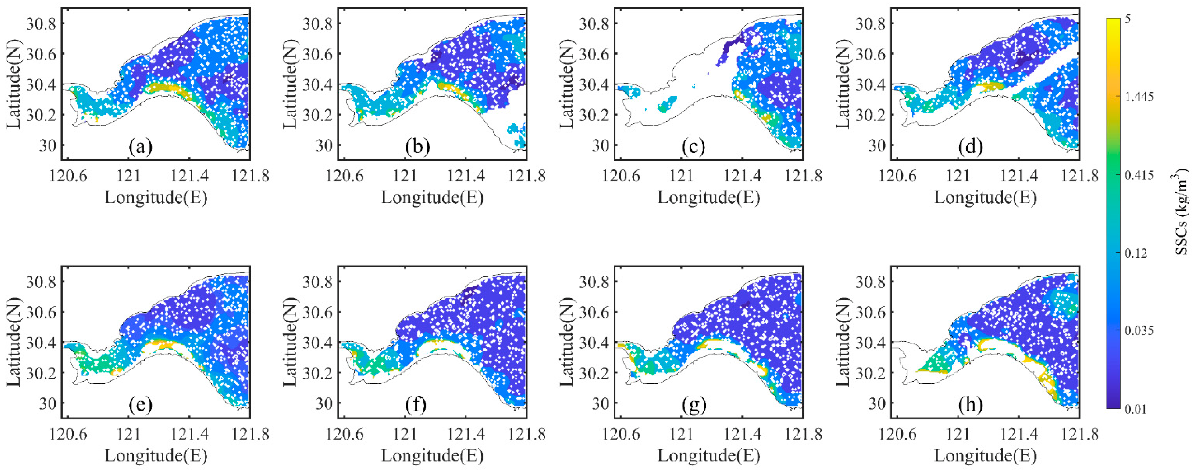
In this paper, the surface SSCs in the Hangzhou Bay retrieved from the GOCI satellite on 24 June 2011 from 0028UTC to 0728UTC with 1 h intervals are selected as the practical observations [11]. The spatial distributions of GOCI-retrieved SSC observations are shown in Figure 1.

Figure 1. Spatial distribution of GOCI-retrieved surface SSCs in the Hangzhou Bay on 24 June 2011, (a) 0028 UTC, (b) 0128 UTC, (c) 0228 UTC, (d) 0328 UTC, (e) 0428 UTC, (f) 0528 UTC, (g) 0628 UTC and (h) 0728 UTC.

2.3. Model Settings

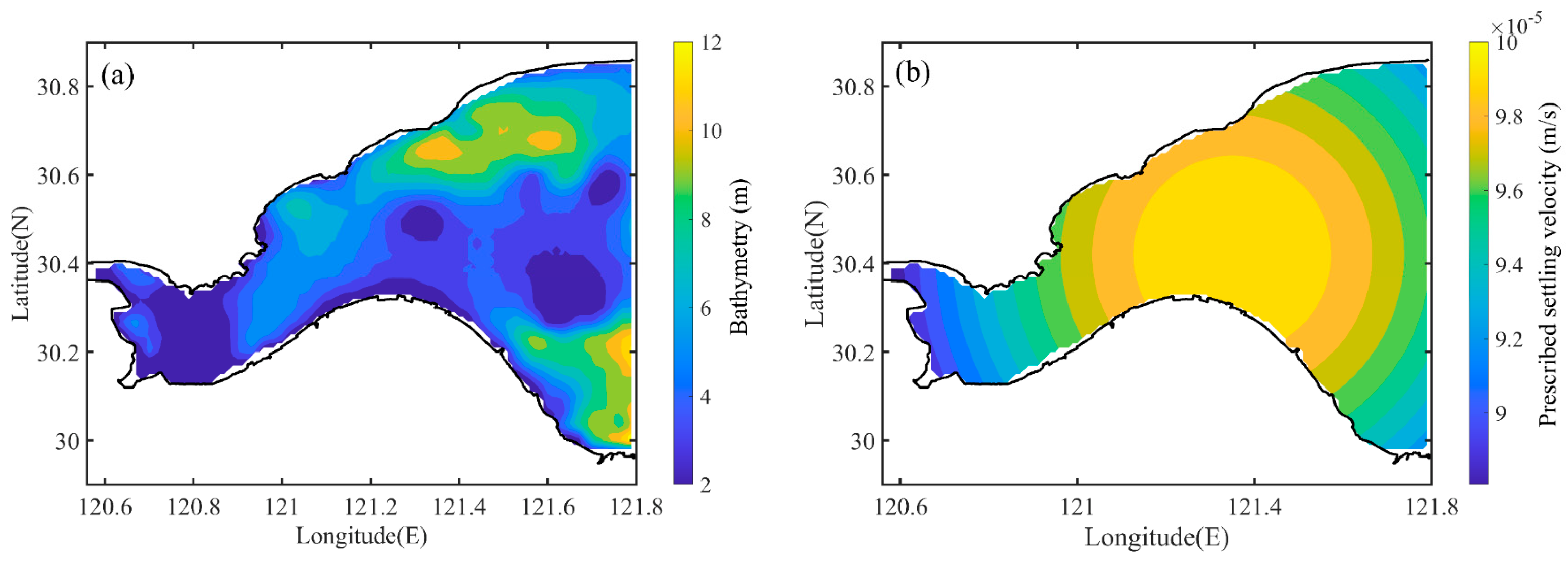
The Hangzhou Bay along the coast of East China Sea is selected as the study area (Figure 2a). The background hydrodynamic field data are interpolated from the FVCOM calculation results [44]. In the hydrodynamic model, four tidal constituents $M_2{,S}_2{,K}_1$ and $O_1$ are set as open boundary conditions in the eastern part of the study area and river boundary conditions are set in the western part of the study area using the multi-year monthly averaged river runoff [13]. As shown in Wang et al. [21], the FVCOM calculation results are in good agreement with the water level and flow velocity observations.

Figure 2. (a) Study area and bathymetry of the Hangzhou Bay, and (b) Spatial distribution of the prescribed settling velocity in twin experiments.

The horizontal resolution of both the three-dimensional suspended cohesive sediment transport model and the adjoint model is 0.01° × 0.01°. The vertical direction is divided into 5 layers. The time step is set to 600 s. The simulation time of twin experiments is 120 hours, and the simulation time of practical experiments is 7 h. The western inflow boundary condition is given by MWRPRC [45]. Referring to Tang [46], the initial value of settling velocity is set to ${1\times 10}^{-4}\mathrm{m/s}$. The initial condition at the surface layer is obtained by interpolating the surface SSCs retrieved from GOCI. According to Wang et al. [33], the initial conditions at other vertical layers are given by multiplying the initial conditions at the surface layer with coefficients (3.5–0.5 k), where k is the number of the layer and the values of k are equal to 1 and 5 for the bottom layer and surface layer, respectively. Referring to Hu et al. [47], the initial value of resuspension rate is set to ${3\times 10}^{–6}\mathrm{m/s}$; in addition, the critical shear stresses for erosion and deposition are equal, and the initial values are set to $0{.4\mathrm{N}/\mathrm{m}}^2$. According to the scale analysis of Wang et al. [33], the horizontal and vertical diffusion coefficients are set to ${80\mathrm{m}}^2/\mathrm{s}$ and ${1\times 10}^{–3}{\mathrm{m}}^2/\mathrm{s}$, respectively.

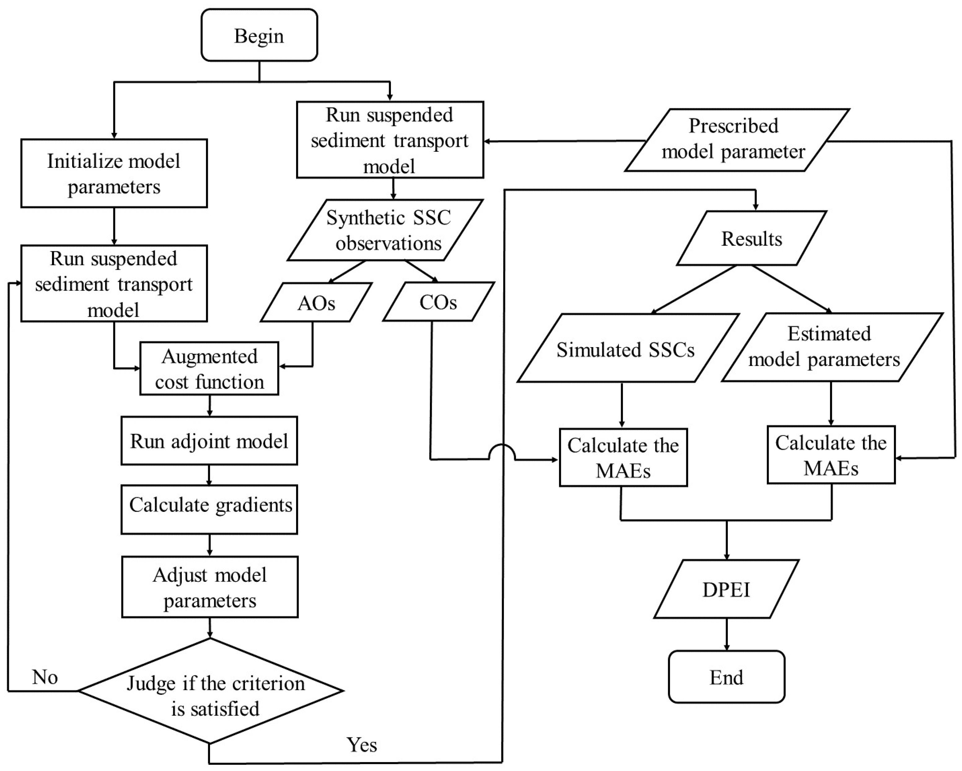
The procedure of conducting the adjoint data assimilation are as follows: the first step is to run the suspended cohesive sediment transport model based on the initial values of the model parameters; the second step is to calculate the corresponding augmented cost function based on the errors between the observations and simulated results, which drive the adjoint model to calculate the adjoint variables; the third step is to calculate the gradient of the augmented cost function with respect to each parameter and adjust the model parameters using the optimization algorithm; finally determine whether the stopping condition is satisfied. If the stopping condition is satisfied, the processes are stopped, while if not, the processes are returned to the first step with the adjusted model parameters. The stopping condition of the processes in this study is that the difference between the normalized augmented cost function in the last two iterations is less than $1{.0\times 10}^{–5}$ with the maximum steps of 50 (500) in the following twin (practical) experiments.

3. Twin Experiments

3.1. Design of Twin Experiments

The twin experiment is an effective method to investigate the effectiveness and accuracy of data assimilation and parameter estimation [33]. The general procedure of a twin experiment is similar to the procedure of the adjoint data assimilation described in Section 2.3, as shown in Figure 3. It is worth noting that the synthetic SSC observations in twin experiments are the simulated hourly surface SSCs obtained by running the suspended cohesive sediment transport model with the prescribed model parameters. Elbern et al. [48] pointed out that the effectiveness of the data assimilation needed to be tested by unassimilated independent observations. In this paper, the synthetic SSC observations are divided into two parts, 10% of the synthetic SSC observations are randomly selected as the check observations (COs) to test the effectiveness of the adjoint data assimilation, and the remaining 90% of the synthetic SSC observations are taken as assimilated observations (AOs), which are assimilated to improve the model simulation results and parameter estimation accuracy.

Figure 3. Flow chart of the twin experiments in this study.

In order to quantitatively analyze the influence of the penalty function method on the performance of the adjoint data assimilation and the accuracy of parameter estimation, the data assimilation and parameter estimation evaluation index (DPEI) in Zhang et al. [34] is introduced, which is calculated as follows:

$$\mathrm{DPEI}=\frac{1}{2}\times \left[\frac{D_{\mathit{COs}}}{{\min (D}_{\mathit{COs}})}+\frac{D_p}{{\min (D}_p)}\right]$$

(18)

where $D_{\mathit{COs}}$ represents the mean absolute errors (MAEs) between COs and the corresponding simulated SSCs; ${\min (D}_{\mathit{COs}})$ is the minimum value of $D_{\mathit{COs}}$ in all the twin experiments; $D_p$ represents the MAEs between the prescribed model parameter and the estimated result; and ${\min (D}_p)$ is the minimum value of $D_p$ in all the twin experiments.

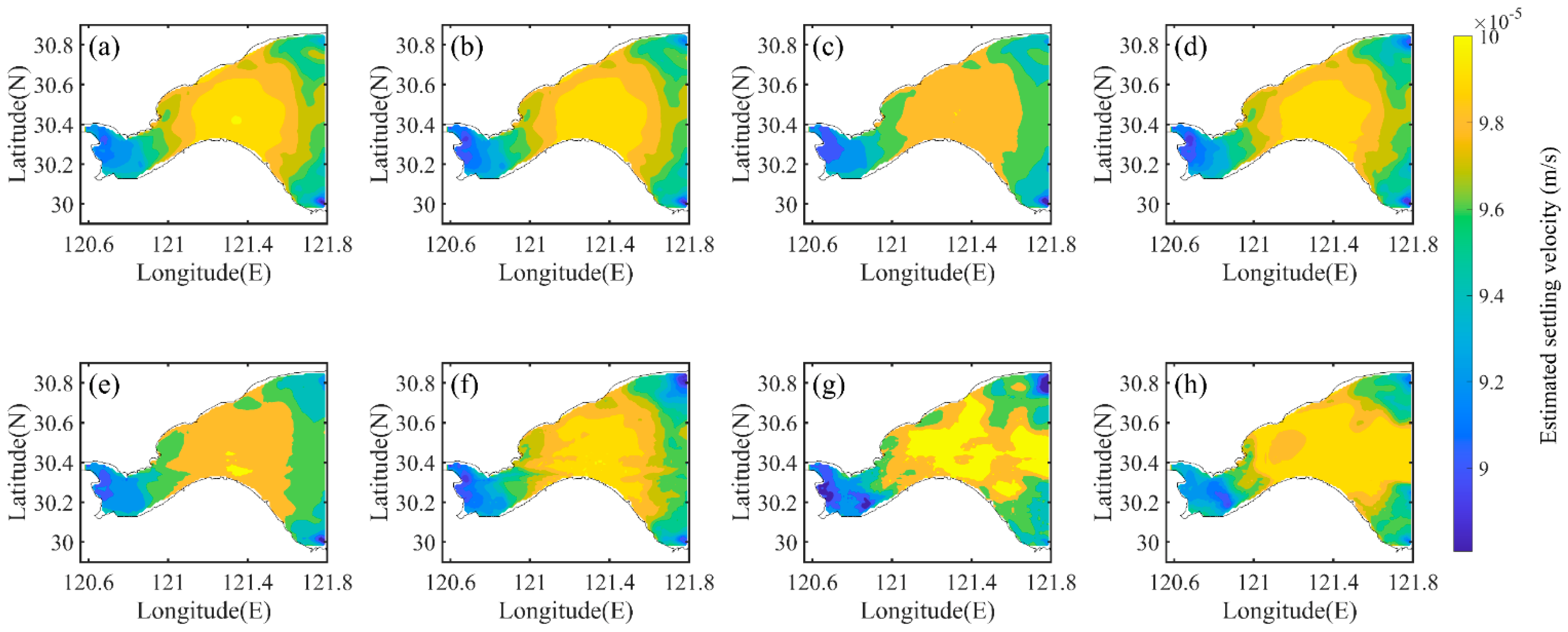
The settling velocity is an important model parameter during the numerical simulation of suspended sediment transport [1]. Therefore, in the twin experiments, only the settling velocity was estimated and the prescribed settling velocity was spatially distributed with the maximum and minimum values of ${1\times 10}^{–4}\mathrm{m/s}$ and $8{.8\times 10}^{–5}\mathrm{m/s}$, respectively, as shown in Figure 2b. The remaining model parameters were set as those described in Section 2.3, and the suspended cohesive sediment transport model was run to obtain the synthetic SSC observations.

In twin experiments TE01 and TE02, the initial guess value of settling velocity was set as ${1\times 10}^{–4}\mathrm{m/s}$. The penalty function method was not applied in TE01, but it was used in TE02 with the maximum and minimum values of ${1\times 10}^{–4}\mathrm{m/s}$ and $8{.8\times 10}^{–5}\mathrm{m/s}$, respectively. The penalty coefficient was set as a constant of ${5\times 10}^7$, according to the selection principle described in Section 2.1.2. In fact, the practical SSC observations are not ideal and have some unavoidable observational errors [25]. Therefore, in twin experiments TE11 and TE12, 0–10% random artificial errors were added into the synthetic SSC observations, and 10−20% (20−30%) random artificial errors were added into the synthetic SSC observations in TE21 and TE22 (TE31 and TE32). The penalty function method was not used in the twin experiments numbered with the suffix of ‘1′, but it was used for those with the suffix of ‘2′. As the augmented cost function may oscillate during the last few iteration steps in the twin experiments, the final result of twin experiments in this study was taken as the better result of the last two iteration steps. The specific designs of the twin experiments are shown in Table 1.

Table 1. Design of twin experiments.

Experiment Number	Random Observational Error	Penalty Function Method
TE01	0	No
TE02	0	Yes
TE11	0–10%	No
TE12	0–10%	Yes
TE21	10–20%	No
TE22	10–20%	Yes
TE31	20–30%	No
TE32	20–30%	Yes

3.2. Twin Experimental Results

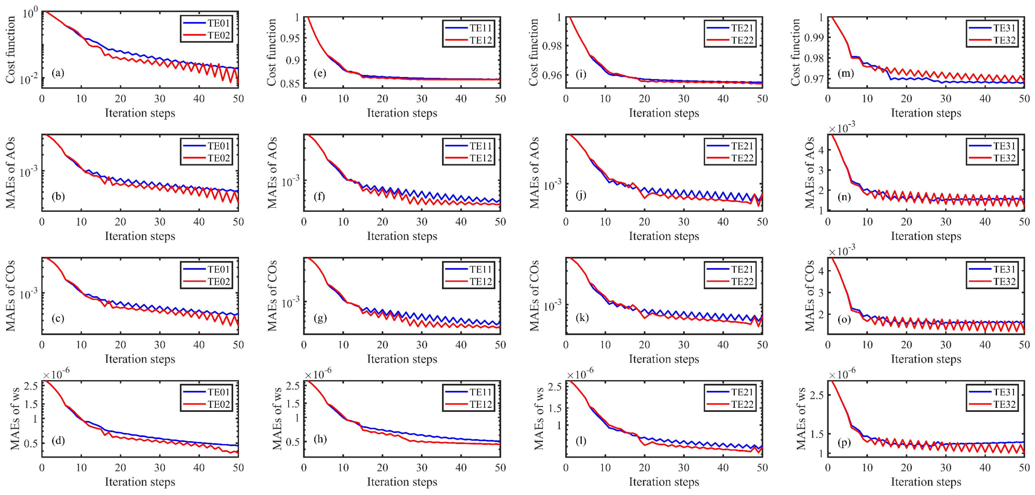
The results of the twin experiments are shown in Figure 4. The normalized cost functions in all the twin experiments gradually decrease with increased iteration steps, and they finally reach the minimum value. The MAEs between AOs and the simulated SSCs also decrease and reach the minimum value, showing the AOs are effectively assimilated. In the absence of observation error (Figure 4 and Table 2), the MAE between COs and the simulated SSCs in TE01 (TE02) decreases from the initial $4{.60\times 10}^{–3}{\mathrm{kg}/\mathrm{m}}^3$ to $4{.04\times 10}^{–4}{\mathrm{kg}/\mathrm{m}}^3$ ($2{.36\times 10}^{–4}{\mathrm{kg}/\mathrm{m}}^3$), with a decrease of 91.22% (94.87%), indicating independently that the assimilation of AOs can improve the model performance. When the artificial observational errors are added into the synthetic SSC observations, the MAEs between COs and the simulated SSCs decrease by 89.30% (90.93%) in TE11 (TE12), 85.02% (89.33%) in TE21 (TE22), and 65.43% (73.91%) in TE31 (TE32), as shown in Figure 4 and Table 2. With the increase of the artificial observational errors, the MAEs for COs are increased, but the MAEs in the experiments with suffix ‘2′ using the penalty function method are less than those in the corresponding experiments with suffix ‘1′. Regardless of the contamination of the synthetic SSC observations from the artificial observational errors, the adjoint data assimilation can always improve the SSC simulation accuracy and the penalty function method can still further improve the effect of the adjoint data assimilation.

Figure 4. In twin experiments, variations of results with iteration steps in TE01 (blue line) and TE02 (red line): (a) normalized cost function, (b) MAEs between AOs and the simulated SSCs, (c) MAEs between COs and the simulated SSCs, (d) MAEs between the prescribed and estimated settling velocity. (e–h) same as (a–d) but for TE11 (blue line) and TE12 (red line), (i–l) same as (a–d) but for TE21 (blue line) and TE22 (red line), (m–p) same as (a–d) but for TE31 (blue line) and TE32 (red line).

Table 2. Results of the normalized cost function, MAEs between AOs and the simulated SSCs, MAEs between COs and the simulated SSCs, MAEs between the prescribed and estimated settling velocity w_s, and DPEI in the twin experiments.

Experiment Number	$\mathbf{MAEs}\mathbf{of}\mathbf{AOs}\left({\mathbf{kg}/\mathbf{m}}^3\right)$		$\mathbf{MAEs}\mathbf{of}\mathbf{COs}\left({\mathbf{kg}/\mathbf{m}}^3\right)$		$\mathbf{MAEs}\mathbf{of}{\mathit{w}}_{\mathit{s}}(\mathbf{m}/\mathbf{s})$		DPEI
	Before	After	Before	After	Before	After
TE01	$4{.76\times 10}^{–3}$	$4{.25\times 10}^{–4}$	$4{.60\times 10}^{–3}$	$4{.04\times 10}^{–4}$	$2{.86\times 10}^{–6}$	$4{.64\times 10}^{–7}$	1.47
TE02	$4{.76\times 10}^{–3}$	$2{.49\times 10}^{–4}$	$4{.60\times 10}^{–3}$	$2{.36\times 10}^{–4}$	$2{.86\times 10}^{–6}$	$3{.77\times 10}^{–7}$	1.00
TE11	$4{.76\times 10}^{–3}$	$5{.17\times 10}^{–4}$	$4{.60\times 10}^{–3}$	$4{.92\times 10}^{–4}$	$2{.86\times 10}^{–6}$	$5{.05\times 10}^{–7}$	1.71
TE12	$4{.76\times 10}^{–3}$	$4{.42\times 10}^{–4}$	$4{.60\times 10}^{–3}$	$4{.17\times 10}^{–4}$	$2{.86\times 10}^{–6}$	$4{.59\times 10}^{–7}$	1.49
TE21	$4{.76\times 10}^{–3}$	$7{.11\times 10}^{–4}$	$4{.60\times 10}^{–3}$	$6{.89\times 10}^{–4}$	$2{.86\times 10}^{–6}$	$6{.15\times 10}^{–7}$	2.28
TE22	$4{.76\times 10}^{–3}$	$4{.93\times 10}^{–4}$	$4{.60\times 10}^{–3}$	$4{.91\times 10}^{–4}$	$2{.86\times 10}^{–6}$	$5{.20\times 10}^{–7}$	1.73
TE31	$4{.76\times 10}^{–3}$	$1{.52\times 10}^{–3}$	$4{.60\times 10}^{–3}$	$1{.59\times 10}^{–3}$	$2{.86\times 10}^{–6}$	$1{.28\times 10}^{–6}$	5.07
TE32	$4{.76\times 10}^{–3}$	$1{.19\times 10}^{–3}$	$4{.60\times 10}^{–3}$	$1{.20\times 10}^{–3}$	$2{.86\times 10}^{–6}$	$1{.00\times 10}^{–6}$	3.87

The MAEs between the prescribed settling velocity and the estimated results of all the twin experiments also gradually decrease and eventually reach the minimum value with increasing iteration steps (Figure 4). Figure 5a,b show the spatial distribution of the estimated settling velocity in TE01 and TE02. The spatial distribution of the estimated settling velocity in TE02 is much closer to the prescribed spatial distribution as shown in Figure 2b than the estimated distribution in TE01. As listed in Table 2, the MAE between the prescribed and estimated settling velocity decreases from the initial $2{.86\times 10}^{–6}\mathrm{m/s}$ ($2{.86\times 10}^{–6}\mathrm{m/s}$) to $4{.64\times 10}^{–7}\mathrm{m/s}$ ($3{.77\times 10}^{–7}\mathrm{m/s}$) in TE01 (TE02), with a decrease of 83.78% (86.82%). When the artificial observational errors are added into the synthetic SSC observations, the spatial distributions of the estimated settling velocity differ significantly from the prescribed distribution (Figure 2b). The results in the experiments using the penalty function method (Figure 5d,f,h), however, are much closer to the spatial distribution of the prescribed settling velocities than those in the experiments without using the penalty function method (Figure 5c,e,g). As listed in Table 2, the MAEs between the prescribed and estimated settling velocity decrease by 82.34% (83.95%) in TE11 (TE12), 78.50% (81.82%) in TE21 (TE22) and 55.24% (65.03%) in TE31 (TE32), showing that the MAEs of settling velocity decrease more in the twin experiments where the penalty function method is used. The above results show that the adjoint data assimilation can estimate the prescribed settling velocity well, and the penalty function method can further improve the accuracy of the parameter estimation.

Figure 5. Spatial distribution of the estimated settling velocity in (a) TE01, (b) TE02, (c) TE11, (d) TE12, (e) TE21, (f) TE22, (g) TE31 and (h) TE32.

To quantitatively evaluate the results of data assimilation and parameter estimation, the DPEI was calculated and is listed in Table 2. When 20%–30% random observational errors are added, the DPEI is 5.07 in TE31, which is much larger than that in TE02. On the other hand, the DPEI is only 3.87 in TE32, showing the effectiveness of the penalty function method. Overall, the penalty function method can improve the comprehensive results of data assimilation and parameter estimation by 31.97% in the absence of observational error. The improvement is 12.87%, 24.12% and 23.67% for adding random observational error into the synthetic SSC observations with percentage range of 0–10, 10–20 and 20–30, respectively.

Overall, no matter whether the synthetic SSC observations are contaminated by the random artificial observational error or not, the prescribed settling velocity can be estimated by assimilating AOs using the adjoint data assimilation. Moreover, both the MAEs for COs and settling velocity and the DPEI in the experiments using the penalty function method are much less than those in the corresponding experiments without using the penalty function method. Thus, the penalty function method can further improve the performance of the adjoint data assimilation.

4. Practical Experiments

4.1. Practical Experiment Design

The effect of the adjoint data assimilation and the penalty function method for improving accuracy of the SSC simulation and the parameter estimation has been demonstrated in twin experiments in Section 3. This section will apply the adjoint data assimilation and the penalty function method in practice. It should be noted that the observations used in the following practical experiments are the GOCI-retrieved SSCs at sea surface (Figure 1), and the rest experimental procedures are the same as the procedures of the adjoint data assimilation described in Section 2.3.

In practical experiments PE11 and PE12, only the settling velocity w_s was estimated by assimilating the GOCI-retrieved SSCs, and the initial guess value of settling velocity was set as ${1\times 10}^{–4}\mathrm{m/s}$. The remaining model parameters were set as described in Section 2.3. The penalty function method was not applied in PE11, but it was used in PE12. According to the variation range of the settling velocity in Wang et al. [21], the maximum and minimum values ($p^{\mathit{max}}$ and $p^{\mathit{min}}$) of settling velocity in the penalty function in PE12 were set as ${3\times 10}^{–4}\mathrm{m/s}$ and $4{.3\times 10}^{–5}\mathrm{m/s}$ through a trial-and-error procedure. The penalty function coefficient was set as a constant of ${9\times 10}^7$ according to the selection principle described in Section 2.1.2.

To further improve the simulation accuracy in practical experiments and explore the general applicability of the penalty function method to other model parameters, two practical experiments PE21 and PE22 were also designed, in which, the spatially varying settling velocity w_s, resuspension rate $M_0$, critical shear stress $\tau$ and initial conditions $C_0$ are simultaneously estimated by assimilating the GOCI-retrieved SSCs. The penalty function method was not used in PE21 and used in PE22. The initial guess values of initial conditions were obtained by interpolating the GOCI-retrieved SSCs, and the initial guess value of resuspension rate (critical shear stress) was set to $3{.0\times 10}^{–6}{\mathrm{kg}/\mathrm{m}}^2/\mathrm{s}$ ($0{.4\mathrm{N}/\mathrm{m}}^2$). The maximum and minimum values of initial conditions in the penalty function method were set as $3{.1\mathrm{kg}/\mathrm{m}}^3$ and $0{.03\mathrm{kg}/\mathrm{m}}^3$, correspondingly. The maximum and minimum values of the resuspension rate (critical shear stress) in the penalty function method were set as ${4\times 10}^{–6}{\mathrm{kg}/\mathrm{m}}^2/\mathrm{s}$ ($0{.2\mathrm{N}/\mathrm{m}}^2$) and ${1\times 10}^{–6}{\mathrm{kg}/\mathrm{m}}^2/\mathrm{s}$ ($1{.2\mathrm{N}/\mathrm{m}}^2$), respectively. According to the principle of selecting penalty function coefficient described in Section 2.1.2, the penalty coefficient for initial conditions, resuspension rate and critical shear stress were set as ${1\times 10}^4$, ${7\times 10}^8$ and ${2\times 10}^4$, respectively. The detailed designs of the practical experiments are shown in Table 3.

Table 3. Design and statistics of practical experiments.

Experiment Number	Penalty Function Method	Estimated Parameters	$\mathbf{MAEs}\mathbf{of}\mathbf{AOs}\left({\mathbf{kg}/\mathbf{m}}^3\right)$		$\mathbf{MAEs}\mathbf{of}\mathbf{COs}\left({\mathbf{kg}/\mathbf{m}}^3\right)$
			Before	After	Before	After
PE11	No	$w_s$	$1{.52\times 10}^{–1}$	$1{.45\times 10}^{–1}$	$1{.53\times 10}^{–1}$	$1{.44\times 10}^{–1}$
PE12	Yes	$w_s$	$1{.52\times 10}^{–1}$	$1{.31\times 10}^{–1}$	$1{.53\times 10}^{–1}$	$1{.30\times 10}^{–1}$
PE21	No	$w_s{,M}_0{,C}_0,\tau$	$1{.52\times 10}^{–1}$	$1{.12\times 10}^{–1}$	$1{.53\times 10}^{–1}$	$1{.17\times 10}^{–1}$
PE22	Yes	$w_s{,M}_0{,C}_0,\tau$	$1{.52\times 10}^{–1}$	$8{.9\times 10}^{–2}$	$1{.53\times 10}^{–1}$	$9{.9\times 10}^{–2}$

4.2. Practical Experiment Results

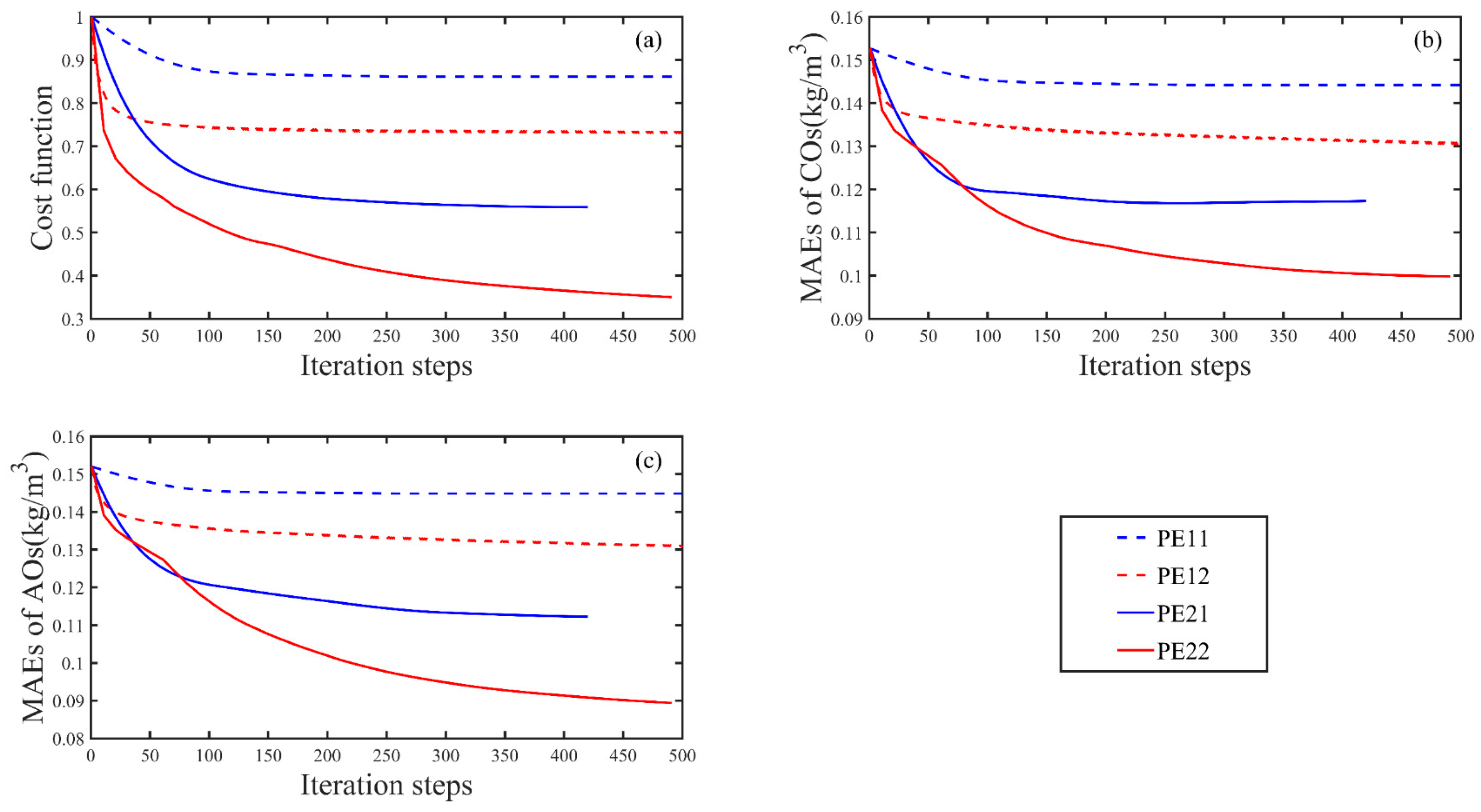
The results of the practical experiments are shown in Figure 6, which show that the normalized cost function and the MAEs for AOs and COs decrease to different degrees, as the number of iteration steps increase. The simulation accuracies of the practical experiments using the penalty function method (PE12 and PE22) are considerably higher than those of the corresponding experiments without using the penalty function method (PE11 and PE21). In detail, as listed in Table 3, the MAE between COs and the simulated SSCs without using the adjoint data assimilation is $1{.53\times 10}^{–1}{\mathrm{kg}/\mathrm{m}}^3$ before data assimilation. The MAE between COs and the simulated SSCs in PE11 (PE12) decreases to $1{.44\times 10}^{–1}{\mathrm{kg}/\mathrm{m}}^3$ ($1{.30\times 10}^{–1}{\mathrm{kg}/\mathrm{m}}^3$), with a decrease of 5.88% (15.03%), showing that the adjoint data assimilation can improve the simulation accuracy evaluated by the independent SSC observations. The MAE between COs and the simulated SSCs in PE21 (PE22) decreases to $1{.17\times 10}^{–1}{\mathrm{kg}/\mathrm{m}}^3$ ($9{.9\times 10}^{–2}{\mathrm{kg}/\mathrm{m}}^3$). This 23.53% (35.29%) decrease indicates that the simultaneous estimation of several model parameters can considerably improve the effect of data assimilation. The penalty function method can further improve the performance of the adjoint data assimilation under both of these scenarios when only the settling velocity is estimated, as well as when the four model parameters are estimated simultaneously.

Figure 6. In practical experiments, variation of results with iteration steps in PE11 (blue dashed line), PE12 (red dashed line), PE21 (blue solid line) and PE22 (red solid line): (a) normalized cost function, (b) MAEs between COs and the simulated SSCs, and (c) MAEs between AOs and the simulated SSCs.

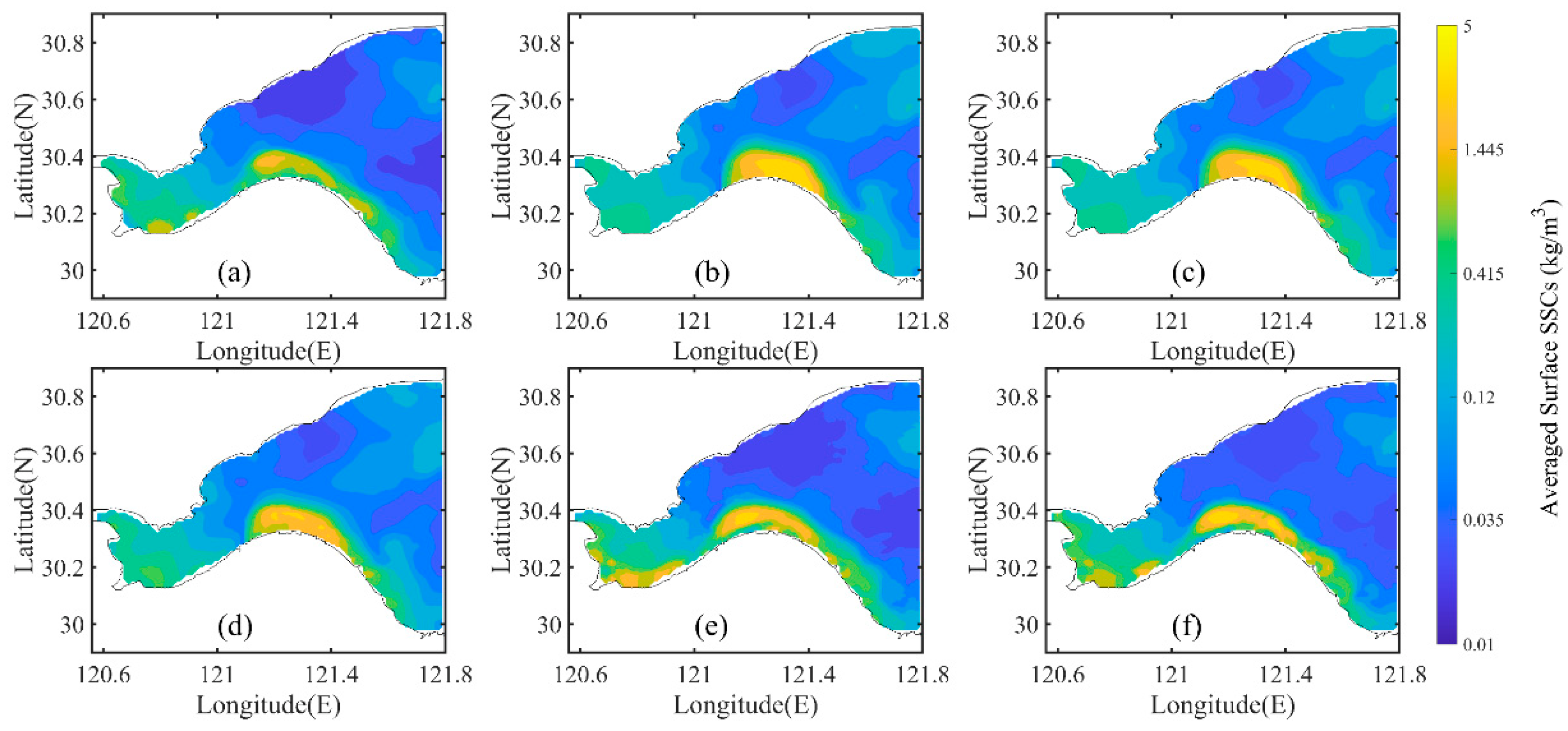
Mostly due to cloud covers, the SSC observations retrieved from GOCI are discontinuous [11], as shown in Figure 1. The hourly GOCI-retrieved SSCs were interpolated and then averaged over the simulation period to obtain spatially continuous SSC observations, as shown in Figure 7a. Figure 7b shows the spatial distribution of the simulated surface SSCs averaged over the simulation period without using the adjoint data assimilation. Figure 7c–f represent the spatial distribution of the simulated surface SSCs in every practical experiment after averaging over the simulation period. It is obvious that the distribution of simulated surface SSCs in PE22 (Figure 7f) is the closest to the actual SSCs observations (Figure 7a). The correlation coefficient between the SSC observations (Figure 7a) and the simulated SSCs without using adjoint data assimilation (Figure 7b) is 0.77, and the correlation coefficient is 0.80 for PE11 (Figure 7c), 0.87 for PE12 (Figure 7d) and 0.91 for both PE21 and PE22 (Figure 7e,f). Moreover, the MAE between the SSC observations (Figure 7a) and the simulated SSCs without using adjoint data assimilation (Figure 7b) is 0.156 kg/m³, and the MAE is 0.141 kg/m³ for PE11 (Figure 7c), 0.110 kg/m³ for PE12 (Figure 7d), 0.096 kg/m³ for PE21 (Figure 7e) and 0.091 kg/m³ for PE22 (Figure 7f). The above results indicate that the adjoint data assimilation with simultaneous estimation of several model parameters can contribute to more accurate modeling of the spatial distribution of surface SSCs. In addition, the penalty function method can further improve the effect of the adjoint data assimilation.

Figure 7. Spatial distribution of temporally averaged SSCs at sea surface: (a) the interpolation results of GOCI-retrieved SSCs, (b) the simulated results without adjoint data assimilation, and the simulated results in (c) PE11, (d) PE12, (e) PE21 and (f) PE22.

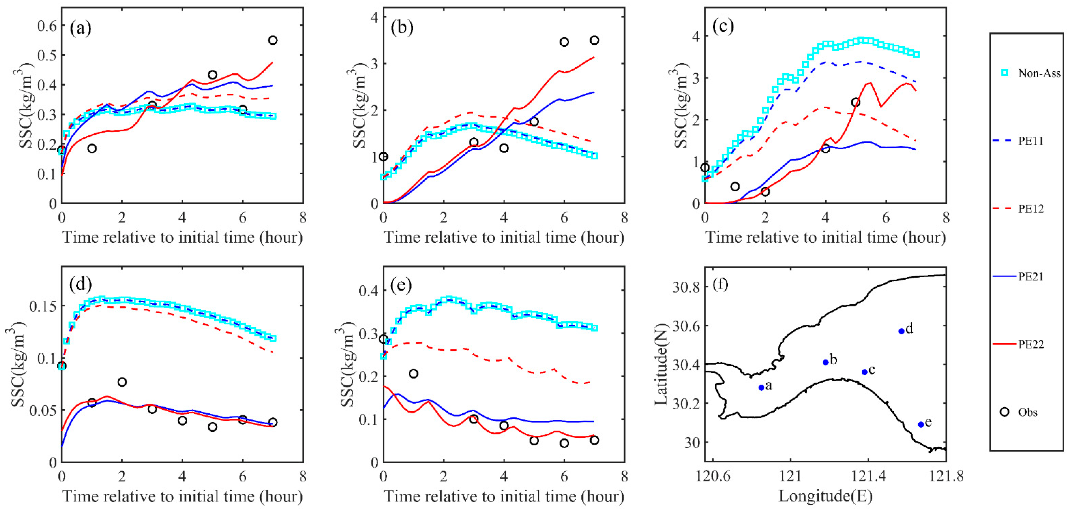
The temporal variations of the simulated and observed SSCs at five unbiased selected points in the Hangzhou Bay are shown in Figure 8. It is apparent that the surface SSCs simulated without using the adjoint data assimilation are far from the observed SSCs at all the five points. While only at point c, the accuracy of the simulated SSCs in PE11 is higher than that without using the adjoint data assimilation (Figure 8c), and the simulated SSCs in PE11 are nearly the same as those simulated without using data assimilation at the other points. At the five randomly selected points, the simulated SSCs in PE12 are closer to the observed SSCs than those in PE11, showing the penalty function method can improve the performance of adjoint data assimilation. However, the differences between the simulated SSCs in PE12 and the observed SSCs at the five points are still large, especially for point b, where the variation trend of the simulated SSCs in PE12 is contrary to the variation trend of SSC observations (Figure 8b). The variation trend and magnitude of the simulated SSCs in PE21 and PE22 are generally consistent with the SSC observations, and the simulation accuracies are significantly higher than those in PE11 and PE12, implying that the simultaneous estimation of multiple model parameters can effectively improve the simulation accuracy of this suspended cohesive sediment transport model. More specifically, during the simulation period, the MAE between the GOCI-retrieved SSCs and the simulated SSCs in PE21 (PE22) is 0.081 kg/m³ (0.056 ${\mathrm{kg}/\mathrm{m}}^3$) at point a, 0.664 ${\mathrm{kg}/\mathrm{m}}^3$(0.528 ${\mathrm{kg}/\mathrm{m}}^3$) at point b, 0.493 ${\mathrm{kg}/\mathrm{m}}^3$ (0.305 ${\mathrm{kg}/\mathrm{m}}^3$) at point c, 0.016 ${\mathrm{kg}/\mathrm{m}}^3$(0.013 ${\mathrm{kg}/\mathrm{m}}^3$) at point d and 0.057 ${\mathrm{kg}/\mathrm{m}}^3$(0.037 ${\mathrm{kg}/\mathrm{m}}^3$) at point e. These values indicate that the penalty function method can improve the effect of the data assimilation to obtain the best simulation results of the temporal variation of the SSCs in the Hangzhou Bay when several model parameters are simultaneously estimated.

Figure 8. Variation of surface SSCs over time at (a) point a, (b) point b, (c) point c, (d) point d and (e) point e: observations (black circles), unassimilated results (cyan squares), PE11 (blue dashed line), PE12 (red dashed line), PE21 (blue solid line) and PE22 (red solid line); (f) Locations of the five randomly selected points.

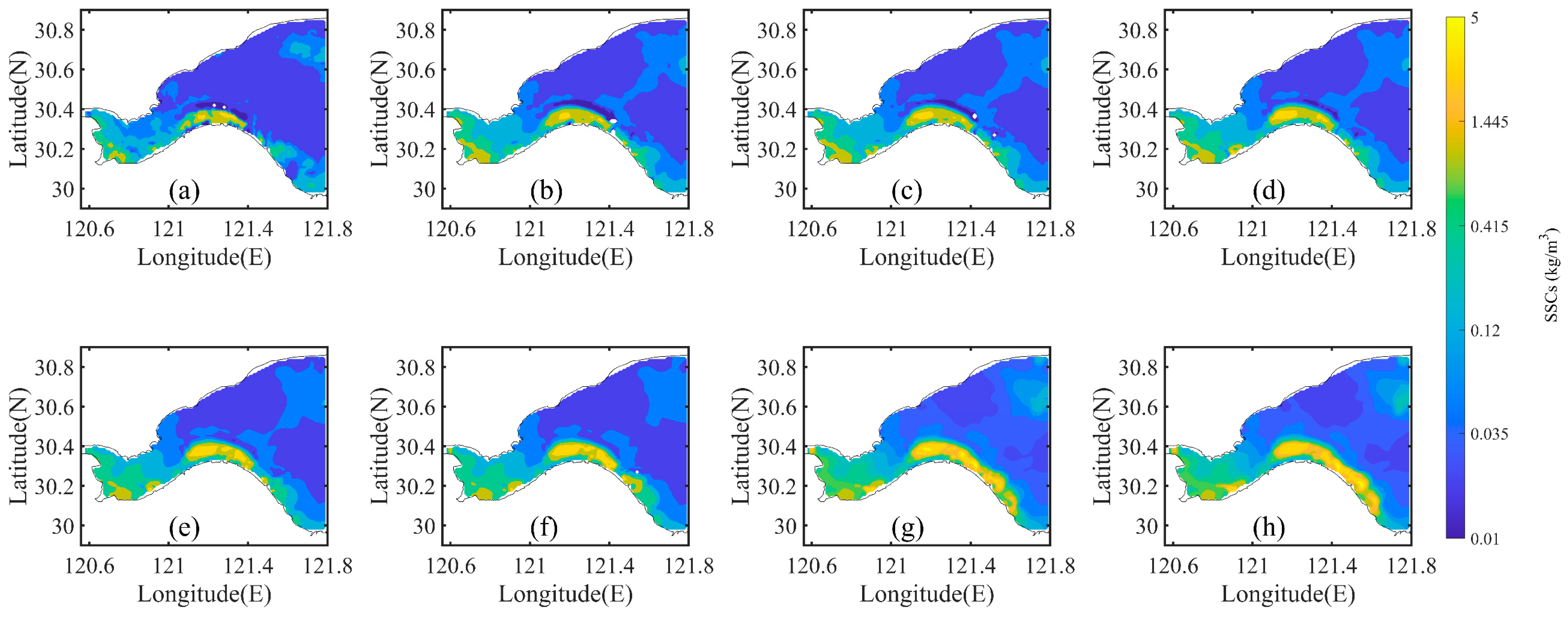
Figure 9 shows the simulated surface SSCs during the period in PE22. It is apparent that the spatial distributions of simulated surface SSCs in PE22 in eight moments during the simulation period (Figure 9a–h) are mostly consistent with GOCI-retrieved SSCs (Figure 1). The correlation coefficients between the spatial distributions of GOCI-retrieved SSCs (Figure 1) and the simulated surface SSCs (Figure 9) in PE22 in the region where the satellite observation data are not missing are 0.76, 0.82, 0.83, 0.92, 0.91, 0.83, 0.81, and 0.91 at 0028UTC−0728UTC, respectively, indicating that the simultaneous estimation of several model parameters with the penalty function method in PE22 can well reproduce the spatial and temporal variations of the GOCI-retrieved SSCs. During the simulation period, the simulated surface SSCs generally high in the west and low in the east in the Hangzhou Bay. The area of high SSCs in the south side of the Hangzhou Bay expands and gradually moves towards the open sea, and the surface SSCs near the river inlet also gradually increase. This SSC distribution indicates that the suspended sediment imported from the river is transported to the open sea with the current. The simulated transport of suspended sediment at the sea surface is basically consistent with that observed by the GOCI data (Figure 1).

Figure 9. Spatial distribution of surface SSCs in PE22 during the simulation period: (a) Simulated result at the initial time, (b–h) Simulated results at each hour interval of the simulation period, respectively.

Overall, in practical experiments, the assimilation of GOCI-retrieved SSCs can improve the model performance of the suspended cohesive sediment transport model. In addition, the penalty function method can further improve the effect of the data assimilation and the simulation accuracy, regardless of the number of model parameters that were estimated. The best simulated results of the SSCs in the Hangzhou Bay are obtained when the key model parameters, including settling velocity, resuspension rate, critical shear stress and initial condition, are simultaneously estimated by assimilating the GOCI-retrieved SSCs with the adjoint data assimilation and the penalty function method.

5. Conclusions

In this paper, based on a three-dimensional suspended cohesive sediment transport model, the transport of the suspended sediment and SSCs in the Hangzhou Bay are simulated by assimilating the GOCI-retrieved SSCs with the adjoint data assimilation. To further improve the effect of data assimilation, the penalty function method, in which the reasonable constraints of the model parameters are added into the adjoint data assimilation, was used. The effectiveness of the combination of the adjoint data assimilation and the penalty function method is evaluated based on the results of the twin experiments and practical experiments.

In the twin experiments, the spatially varying settling velocity is prescribed, then the suspended cohesive sediment transport model is run to obtain the synthetic SSC observations. The spatially varying settling velocity is estimated by assimilating the synthetic SSC observations with different ranges of random artificial errors to investigate the effectiveness of the adjoint data assimilation and the penalty function method. In all the twin experiments, the MAEs between the COs and the corresponding simulated SSCs and the MAEs between the prescribed and estimated settling velocity are greatly reduced (Figure 4). The spatial distributions of the estimated settling velocity using the penalty function method are much closer to the prescribed settling velocity (Figure 5). The calculated DPEI show that the penalty function method can improve the performance of adjoint data assimilation by 31.97% in the absence of observational error, and can also improve the performance of adjoint data assimilation when the synthetic SSC observations are contaminated by the random artificial errors (Table 2). Overall, regardless of the contamination of the synthetic SSC observations by the random artificial errors, the adjoint data assimilation can improve the simulation accuracy of the suspended sediment transport model. The penalty function method can further improve the performance of the adjoint data assimilation and parameter estimation.

In the practical experiments, the spatially varying settling velocity is estimated by assimilating the GOCI-retrieved SSCs. The results show that the simulation accuracy of the SSCs in the Hangzhou Bay can be improved by the adjoint data assimilation. The penalty function method can further reduce the MAE between the COs and the corresponding simulated SSCs from 1.44 × 10^–1 kg/m³ to 1.30 × 10^–1 kg/m³, but the differences between the COs and the corresponding simulated SSCs are still large. In order to further improve the simulation accuracy, the model parameters, including the spatially varying settling velocity, resuspension rate, initial conditions and critical shear stress, are simultaneously estimated in the practical experiments. Compared with the practical experiments only estimating settling velocity in PE11 and PE12, the MAEs between the COs and the simulated SSCs decrease more in practical experiments PE21 and PE22 with simultaneously estimating multiple model parameters (Figure 6). Moreover, the best model performance is obtained in practical experiment PE22, where the penalty function method is introduced into the adjoint data assimilation. The simulated results in PE22 well reproduce the spatial and temporal variation of suspended sediment in the Hangzhou Bay (Figure 7 and Figure 8), and the variations of the simulated SSCs in the Hangzhou Bay caused by suspended sediment transport are also basically consistent with the GOCI-retrieved SSCs (Figure 1).

In summary, this study demonstrates that adjoint data assimilation can improve the simulation accuracy of the suspended sediment transport model and the precision of parameter estimation; moreover, the penalty function method can further improve the effect of the adjoint data assimilation. Although the exact parameter values may vary at different locations, the procedures proposed in this study to improve the accuracy of modeling SSC can be applied at many other estuaries around the world.

References

- Yang, X.; Mao, Z.; Huang, H.; Zhu, Q. Using GOCI retrieval data to initialize and validate a sediment transport model for monitoring diurnal variation of SSC in Hangzhou Bay, China. Water 2016, 8, 108. [Google Scholar] [CrossRef]
- Martin, J.-M.; Windom, H.L. Present and future roles of ocean margins in regulating marine biogeochemical cycles of trace elements. In Proceedings of the Dahlem Workshop on Ocean Margin Processes in Global Change, Chichester, UK, 18 March 1990; pp. 45–67. [Google Scholar]
- Ilyina, T.; Pohlmann, T.; Lammel, G.; Sündermann, J. A fate and transport ocean model for persistent organic pollutants and its application to the North Sea. J. Mar. Syst. 2006, 63, 1–19. [Google Scholar] [CrossRef]
- Fan, D.; Tu, J.; Shang, S.; Cai, G. Characteristics of tidal-bore deposits and facies associations in the Qiantang Estuary, China. Mar. Geol. 2014, 348, 1–14. [Google Scholar] [CrossRef]
- Hu, Y.; Yu, Z.; Zhou, B.; Li, Y.; Yin, S.; He, X.; Peng, X.; Shum, C.K. Tidal-driven variation of suspended sediment in Hangzhou Bay based on GOCI data. Int. J. Appl. Earth Obs. Geoinf. 2019, 82, 101920. [Google Scholar] [CrossRef]
- Cai, L.; Zhou, M.; Liu, J.; Tang, D.; Zuo, J. HY-1C observations of the impacts of islands on suspended sediment distribution in Zhoushan coastal waters, China. Remote Sens. 2020, 12, 1766. [Google Scholar] [CrossRef]
- Wren, D.; Barkdoll, B.D.; Kuhnle, R.A.; Derrow, R.W. Field techniques for suspended-sediment measurement. J. Hydraul. Eng. 2000, 126, 97–104. [Google Scholar] [CrossRef]
- Hamilton, L.J.; Shi, Z.; Zhang, S.Y. Acoustic backscatter measurements of estuarine suspended cohesive sediment concentration profiles. J. Coast. Res. 1998, 14, 1213–1224. [Google Scholar]
- Eleveld, M.A.; Pasterkamp, R.; van der Woerd, H.J.; Pietrzak, J.D. Remotely sensed seasonality in the spatial distribution of sea-surface suspended particulate matter in the southern North Sea. Estuar. Coast. Shelf Sci. 2008, 80, 103–113. [Google Scholar] [CrossRef]
- Li, J.; Gao, S.; Wang, Y. Delineating suspended sediment concentration patterns in surface waters of the Changjiang Estuary by remote sensing analysis. Acta Oceanol. Sin. 2010, 29, 38–47. [Google Scholar] [CrossRef]
- He, X.; Bai, Y.; Pan, D.; Huang, N.; Dong, X.; Chen, J.; Chen, C.-T.A.; Cui, Q. Using geostationary satellite ocean color data to map the diurnal dynamics of suspended particulate matter in coastal waters. Remote Sens. Environ. 2013, 133, 225–239. [Google Scholar] [CrossRef]
- Choi, J.-K.; Park, Y.J.; Lee, B.R.; Eom, J.; Moon, J.-E.; Ryu, J.-H. Application of the Geostationary Ocean Color Imager (GOCI) to mapping the temporal dynamics of coastal water turbidity. Remote Sens. Environ. 2014, 146, 24–35. [Google Scholar] [CrossRef]
- Du, Y.; Lin, H.; He, S.; Wang, D.; Wang, Y.P.; Zhang, J. Tide-Induced Variability and Mechanisms of Surface Suspended Sediment in the Zhoushan Archipelago along the Southeastern Coast of China Based on GOCI Data. Remote Sens. 2021, 13, 929. [Google Scholar] [CrossRef]
- Gerber, F.; de Jong, R.; Schaepman, M.E.; Schaepman-Strub, G.; Furrer, R. Predicting missing values in spatio-temporal remote sensing data. IEEE Trans. Geosci. Remote Sens. 2018, 56, 2841–2853. [Google Scholar] [CrossRef]
- Tian, L.; Sun, X.; Li, J.; Xing, Q.; Song, Q.; Tong, R. Sampling Uncertainties of Long-Term Remote-Sensing Suspended Sediments Monitoring over China’s Seas: Impacts of Cloud Coverage and Sediment Variations. Remote Sens. 2020, 12, 1945. [Google Scholar] [CrossRef]
- Lin, B.; Falconer, R.A. Numerical modelling of three-dimensional suspended sediment for estuarine and coastal waters. J. Hydraul. Res. 1996, 34, 435–456. [Google Scholar] [CrossRef]
- Cancino, L.; Neves, R. Hydrodynamic and sediment suspension modelling in estuarine systems: Part I: Description of the numerical models. J. Mar. Syst. 1999, 22, 105–116. [Google Scholar] [CrossRef]
- Wang, X.H. Tide-induced sediment resuspension and the bottom boundary layer in an idealized estuary with a muddy bed. J. Phys. Oceanogr. 2002, 32, 3113–3131. [Google Scholar] [CrossRef]
- Nguyen, K.D.; Guillou, S.; Chauchat, J.; Barbry, N. A two-phase numerical model for suspended-sediment transport in estuaries. Adv. Water Resour. 2009, 32, 1187–1196. [Google Scholar] [CrossRef]
- Amoudry, L.O.; Souza, A.J. Deterministic coastal morphological and sediment transport modeling: A review and discussion. Rev. Geophys. 2011, 49, RG2002. [Google Scholar] [CrossRef]
- Wang, D.; Zhang, J.; He, X.; Chu, D.; Lv, X.; Wang, Y.P.; Yang, Y.; Fan, D.; Gao, S. Parameter estimation for a cohesive sediment transport model by assimilating satellite observations in the Hangzhou Bay: Temporal variations and spatial distributions. Ocean Model. 2018, 121, 34–48. [Google Scholar] [CrossRef]
- Wang, X.; Pinardi, N. Modeling the dynamics of sediment transport and resuspension in the northern Adriatic Sea. J. Geophys. Res. Ocean. 2002, 107, 18-1–18-23. [Google Scholar] [CrossRef]
- Guan, W.B.; Kot, S.C.; Wolanski, E. 3-D fluid-mud dynamics in the Jiaojiang Estuary, China. Estuar. Coast. Shelf Sci. 2005, 65, 747–762. [Google Scholar] [CrossRef]
- Teisson, C. Cohesive suspended sediment transport: Feasibility and limitations of numerical modeling. J. Hydraul. Res. 1991, 29, 755–769. [Google Scholar] [CrossRef]
- Yang, Z.; Hamrick, J.M. Variational inverse parameter estimation in a cohesive sediment transport model: An adjoint approach. J. Geophys. Res. Ocean. 2003, 108, 3055. [Google Scholar] [CrossRef]
- Fringer, O.B.; Dawson, C.N.; He, R.; Ralston, D.K.; Zhang, Y.J. The future of coastal and estuarine modeling: Findings from a workshop. Ocean Model. 2019, 143, 101458. [Google Scholar] [CrossRef]
- Navon, I.M. Practical and theoretical aspects of adjoint parameter estimation and identifiability in meteorology and oceanography. Dyn. Atmos. Ocean. 1998, 27, 55–79. [Google Scholar] [CrossRef]
- Carton, J.A.; Chepurin, G.; Cao, X.; Giese, B. A simple ocean data assimilation analysis of the global upper ocean 1950–95. Part I: Methodology. J. Phys. Oceanogr. 2000, 30, 294–309. [Google Scholar] [CrossRef]
- Pleskachevsky, A.; Gayer, G.; Horstmann, J.; Rosenthal, W. Synergy of satellite remote sensing and numerical modeling for monitoring of suspended particulate matter. Ocean Dyn. 2005, 55, 2–9. [Google Scholar] [CrossRef]
- Stroud, J.R.; Lesht, B.M.; Schwab, D.J.; Beletsky, D.; Stein, M.L. Assimilation of satellite images into a sediment transport model of Lake Michigan. Water Resour. Res. 2009, 45. [Google Scholar] [CrossRef]
- El Serafy, G.Y.; Eleveld, M.A.; Blaas, M.; van Kessel, T.; Aguilar, S.G.; Van der Woerd, H.J. Improving the description of the suspended particulate matter concentrations in the southern North Sea through assimilating remotely sensed data. Ocean Sci. J. 2011, 46, 179–204. [Google Scholar] [CrossRef]
- Margvelashvili, N.; Andrewartha, J.; Herzfeld, M.; Robson, B.J.; Brando, V.E. Satellite data assimilation and estimation of a 3D coastal sediment transport model using error-subspace emulators. Environ. Model. Softw. 2013, 40, 191–201. [Google Scholar] [CrossRef]
- Wang, D.; Cao, A.; Zhang, J.; Fan, D.; Liu, Y.; Zhang, Y. A three-dimensional cohesive sediment transport model with data assimilation: Model development, sensitivity analysis and parameter estimation. Estuar. Coast. Shelf Sci. 2018, 206, 87–100. [Google Scholar] [CrossRef]
- Zhang, J.; Chu, D.; Wang, D.; Cao, A.; Lv, X.; Fan, D. Estimation of spatially varying parameters in three-dimensional cohesive sediment transport models by assimilating remote sensing data. J. Mar. Sci. Technol. 2018, 23, 319–332. [Google Scholar] [CrossRef]
- Polyak, V.T.; Tret’yakov, N.V. The method of penalty estimates for conditional extremum problems. USSR Comput. Math. Math. Phys. 1973, 13, 42–58. [Google Scholar] [CrossRef]
- Smith, A.E.; Coit, D.W.; Baeck, T.; Fogel, D.; Michalewicz, Z. Penalty functions. Handb. Evol. Comput. 1997, 97, C5. [Google Scholar]
- Zhu, Y.; Navon, I.M. Impact of parameter estimation on the performance of the FSU global spectral model using its full-physics adjoint. Mon. Weather Rev. 1999, 127, 1497–1517. [Google Scholar] [CrossRef]
- Cai, G.; Selesnick, I.W.; Wang, S.; Dai, W.; Zhu, Z. Sparsity-enhanced signal decomposition via generalized minimax-concave penalty for gearbox fault diagnosis. J. Sound Vib. 2018, 432, 213–234. [Google Scholar] [CrossRef]
- Partheniades, E. Erosion and deposition of cohesive soils. J. Hydraul. Div. 1965, 91, 105–139. [Google Scholar] [CrossRef]
- Nour-Omid, B.; Wriggers, P. A note on the optimum choice for penalty parameters. Commun. Appl. Numer. Methods 1987, 3, 581–585. [Google Scholar] [CrossRef]
- Coello, C.A.C. Theoretical and numerical constraint-handling techniques used with evolutionary algorithms: A survey of the state of the art. Comput. Methods Appl. Mech. Eng. 2002, 191, 1245–1287. [Google Scholar] [CrossRef]
- Ryu, J.H.; Choi, J.K.; Eom, J.; Ahn, J.H. Temporal variation in Korean coastal waters using geostationary ocean color imager. J. Coast. Res. 2011, 64, 1731–1735. [Google Scholar]
- Ryu, J.H.; Han, H.J.; Cho, S.; Park, Y.J.; Ahn, Y.H. Overview of geostationary ocean color imager (GOCI) and GOCI data processing system (GDPS). Ocean Sci. J. 2012, 47, 223–233. [Google Scholar] [CrossRef]
- Chen, C.; Liu, H.; Beardsley, R.C. An unstructured grid, finite-volume, three-dimensional, primitive equations ocean model: Application to coastal ocean and estuaries. J. Atmos. Ocean. Technol. 2003, 20, 159–186. [Google Scholar] [CrossRef]
- MWRPRC (the Ministry of Water Resource of the People’s Republic of China). Bulletin of Chinese Rivers and Sediments 2011; China Water Power Press: Beijing, China, 2011. [Google Scholar]
- Tang, J.H. Characteristics of Fine Cohesive Sediment’s Flocculation in the Changjiang Estuary and Its Adjacent Sea Area. Master’s Thesis, East China Normal University, Shanghai, China, 2007. [Google Scholar]
- Hu, K.; Ding, P.; Wang, Z.; Yang, S. A 2D/3D hydrodynamic and sediment transport model for the Yangtze Estuary, China. J. Mar. Syst. 2009, 77, 114–136. [Google Scholar] [CrossRef]
- Elbern, H.; Strunk, A.; Schmidt, H.; Talagrand, O. Emission rate and chemical state estimation by 4-dimensional variational inversion. Atmos. Chem. Phys. 2007, 7, 3749–3769. [Google Scholar] [CrossRef]
Disclaimer/Publisher’s Note: The statements, opinions and data contained in all publications are solely those of the individual author(s) and contributor(s) and not of MDPI and/or the editor(s). MDPI and/or the editor(s) disclaim responsibility for any injury to people or property resulting from any ideas, methods, instructions or products referred to in the content. |
© 2022 by the authors. Licensee MDPI, Basel, Switzerland. This article is an open access article distributed under the terms and conditions of the Creative Commons Attribution (CC BY) license (https://creativecommons.org/licenses/by/4.0/).