Article

Siam-Sort: Multi-Target Tracking in Video SAR Based on Tracking by Detection and Siamese Network

National Laboratory of Radar Signal Processing, Xidian University, Xi’an 710071, China
*
Author to whom correspondence should be addressed.
Remote Sens. 2023, 15(1), 146; https://doi.org/10.3390/rs15010146
Submission received: 17 November 2022 / Revised: 20 December 2022 / Accepted: 22 December 2022 / Published: 27 December 2022
(This article belongs to the Section Remote Sensing Image Processing)

Abstract

:
Shadows are widely used in the tracking of moving targets by video synthetic aperture radar (video SAR). However, they always appear in groups in video SAR images. In such cases, track effects produced by existing single-target tracking methods are no longer satisfactory. To this end, an effective way to obtain the capability of multiple target tracking (MTT) is in urgent demand. Note that tracking by detection (TBD) for MTT in optical images has achieved great success. However, TBD cannot be utilized in video SAR MTT directly. The reasons for this is that shadows of moving target are quite different from in video SAR image than optical images as they are time-varying and their pixel sizes are small. The aforementioned characteristics make shadows in video SAR images hard to detect in the process of TBD and lead to numerous matching errors in the data association process, which greatly affects the final tracking performance. Aiming at the above two problems, in this paper, we propose a multiple target tracking method based on TBD and the Siamese network. Specifically, to improve the detection accuracy, the multi-scale Faster-RCNN is first proposed to detect the shadows of moving targets. Meanwhile, dimension clusters are used to accelerate the convergence speed of the model in the training process as well as to obtain better network weights. Then, SiamNet is proposed for data association to reduce matching errors. Finally, we apply a Kalman filter to update the tracking results. The experimental results on two real video SAR datasets demonstrate that the proposed method outperforms other state-of-art methods, and the ablation experiment verifies the effectiveness of multi-scale Faster-RCNN and SimaNet.

1. Introduction

Video synthetic aperture radar (video SAR) has been a research hotspot owing to its advantages of high resolution and high rate. It is not only able to work in all-weather and all-day conditions like conventional SAR can, but it also allows for monitoring an area of interest continuously. Therefore, video SAR can be used for moving target tracking.
However, moving targets are unfocused and shifted in video SAR images due to the Doppler translation caused by the relative motion between the radar and the moving targets [1]. Thus, it is impossible to track moving targets directly in video SAR images. Nevertheless, the imaging characteristics of the moving target lead to a low-energy area at its real imaging position, which is shown as a shadow in the video SAR image. Ynal et al. [2] detailed the generation mechanism of shadows of moving targets and analyzed their characteristics, finally giving a formula to calculate the shadow size. Miller et al. [3] discussed the impact of the video SAR system’s imaging parameters on shadows of moving targets. The above articles illustrate that the shadow of a moving target can reflect its position and size in the video SAR image. Hence, a feasible idea is that tracking the moving target can be achieved by tracking its shadow.
Some scholars have proposed tracking methods based on the shadows of moving targets in video SAR images. Xu et al. introduced a method that detects moving targets using piecewise convolutional neural networks (PCNN) and tracks targets based on KCF [4]. Yang et al. proposed a tracking and refocusing framework for ground moving targets in video SAR [5]. A method for target detection and tracking that uses a geographic information system (GIS) map and a convolutional neural network (CNN) is introduced in [6]. However, these single-target-tracking methods cannot be applied to real scenes with multiple moving targets of interest, as shown in Figure 1, due to their quite long runtime and horrible tracking performance in these cases.
Therefore, there is an urgent demand to achieve multi-target tracking (MTT) in video SAR images. However, few scholars have researched this technology. Note, however, that the related research has resulted in advancements in optical images. Tracking in optical imafes is greatly boosted by the application of tracking by detection (TBD) [7,8,9,10]. TBD involves three components, namely, target detection, data association, and target tracking. Among them, target detection is used to obtain target observations such as the locations and sizes in the current scene. Data association is a process that assigns the observations to multiple previously known or identified moving targets, and target tracking implements the tracking for each moving target based on the matched observations. Bewley et al. [7] proposed a simple online and real-time tracking method (SORT) based on TBD in 2016. It achieves good tracking performance by using the Hungarian algorithm [11] for data association and applying a Kalman filter [12] to obtain the tracking results of the targets. Nevertheless, its tracking performance will deteriorate when the uncertainty of the target’s state estimation is low. The reason for this is that SORT only uses the motion characteristics of targets for data association. In recent years, convolutional neural networks (CNN) have been widely used in computer vision [13,14,15,16] for their remarkable representation abilities. On this basis, Wojke et al. improved SORT and proposed a simple online and real-time tracking method with a deep association metric (Deep SORT) [8]. It adopted a CNN-based method to detect targets and used target features extracted by the re-identification network for data association, which improved the robustness of the method.
Inspired by the successful application of TBD in optical images, we introduce it for MTT in video SAR images. However, its direct application is problematic. Unlike optical images, the shadows of moving targets in video SAR images are time-varying, and their sizes are small. These characteristics cause the target shadows to be difficult to detect and lead to many matching errors in the data association process, which seriously deteriorates the final tracking performance. Therefore, to solve these problems, we propose a novel TBD-based method, Siam-Sort, for MTT in video SAR images. Specifically, we first propose multi-scale Faster-RCNN to improve the detection accuracy for moving target shadows. Then, to reduce matching errors, SiamNet, based on the Siamese network, is proposed, which uses the similarities between features of target shadows and features of observations to achieve data association. The major contributions of our method are indicated as follows:
  • Multi-scale Faster-RCNN is proposed to detect the shadows of moving targets. We modify the feature extractor of Faster-RCNN where the multi-layer features of the network are fused to enhance its feature representation capability. Moreover, we predict the target shadows on the feature maps of multiple scales to improve the detection accuracy.
  • We utilize dimension clusters to optimize the generation strategy of the anchors for multi-scale faster-RCNN and to speed up the convergence speed of the model in the training process, which further improves the detection performance of multi-scale faster-RCNN.
  • SiamNet is proposed for data association. We first extract the features of target shadows and observations. Then, we calculate the similarities between their features to build the similarity matrix. Finally, the matrix is used by the Hungarian algorithm to match the targets and observations. Compared with other methods, it significantly reduces the matching errors.
The rest of this article is organized as follows. Section 2 introduces the multi-scale faster-RCNN, SiamNet, and overall tracking process in detail. Section 3 shows the results of the proposed method on two real video SAR datasets. Section 4 discusses some particulars of the proposed method and provides the ablation experiments for multi-scale Faster-RCNN and SiamNet. Section 5 concludes the article.

2. Methodology

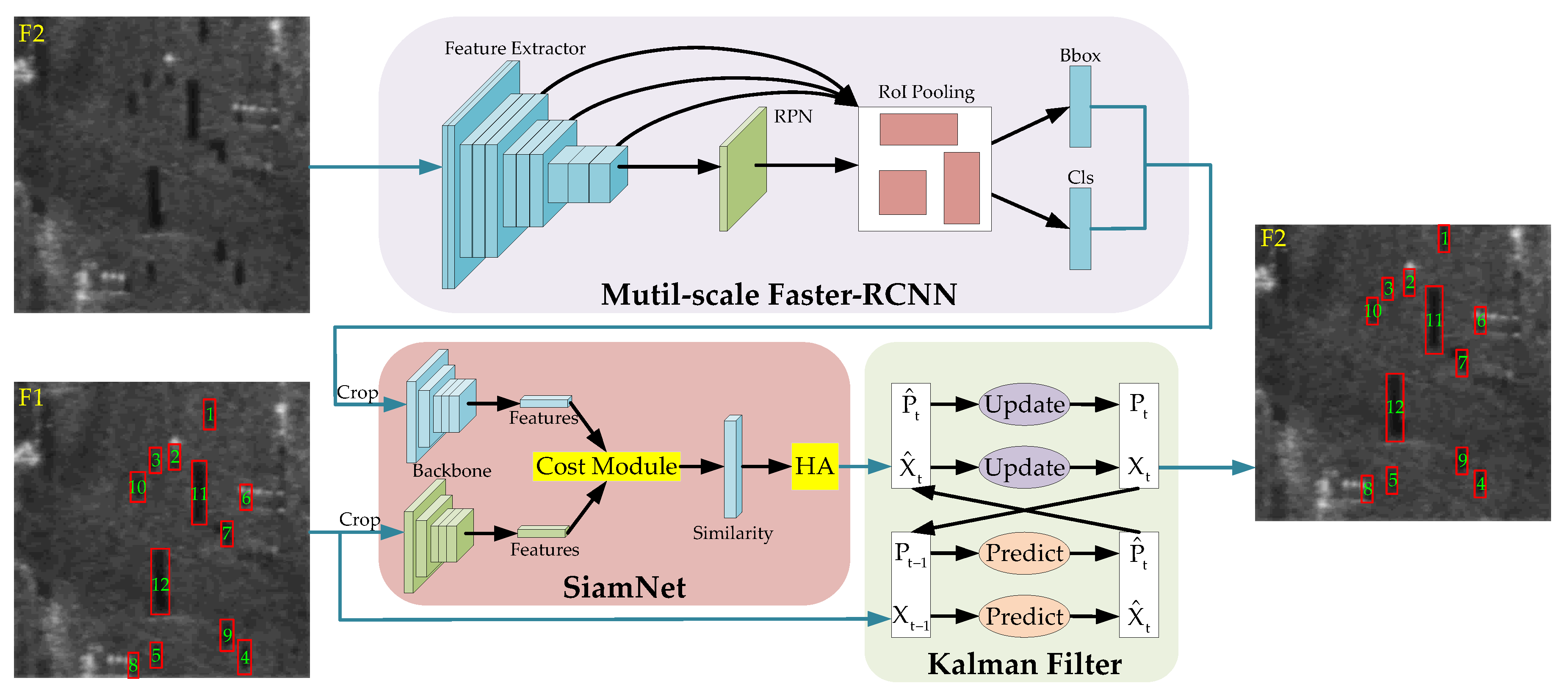
The framework of Siam-sort for MTT in video SAR is shown in Figure 2. It consists of multi-scale Faster-RCNN, SiamNet, and a Kalman filter, which correspond to target detection, data association, and target tracking of TBD, respectively.
When Siam-sort is used to track multiple targets in video-SAR, it receives two consecutive frames, F1 and F2, where F1 is the template frame and F2 is the search frame. Siam-sort first utilizes multi-scale Faster-RCNN to detect the moving target shadows in search frame F2, and the detection results are recorded as the observations of moving targets. Then, Siam-sort crops out patches of the observations in F2. In the same way, Siam-sort crops out patches of the moving targets in F1. Next, Siam-sort takes the patches of the observations and moving targets into the two input branches of SiamNet and calculates the similarities between them to assign the observations to the moving targets. Finally, Siam-sort uses the matched observations to predict and update the tracking results of each moving target via a Kalman filter.
To reduce the computing capacity and matching errors, all patches of observations are grouped according to their classes and then grouped again based on the Mahalanobis distance [17] between the target and the observation before SiamNet is used. Furthermore, Siam-sort saves patches of real moving targets in all frames and matches them with the patches of the observations in the search frame by using SiamNet to perform re-tracking in the case that observations are missing in several consecutive frames.
Siam-sort always uses the tracking result of the previous frame as one of the inputs for target tracking in the current frame. By applying the above operation to the whole video SAR image sequence, we achieve multiple target tracking in video SAR. In the following, we will introduce the implementation and tracking process of Siam-sort in detail.

2.1. Multi-Scale Faster-RCNN

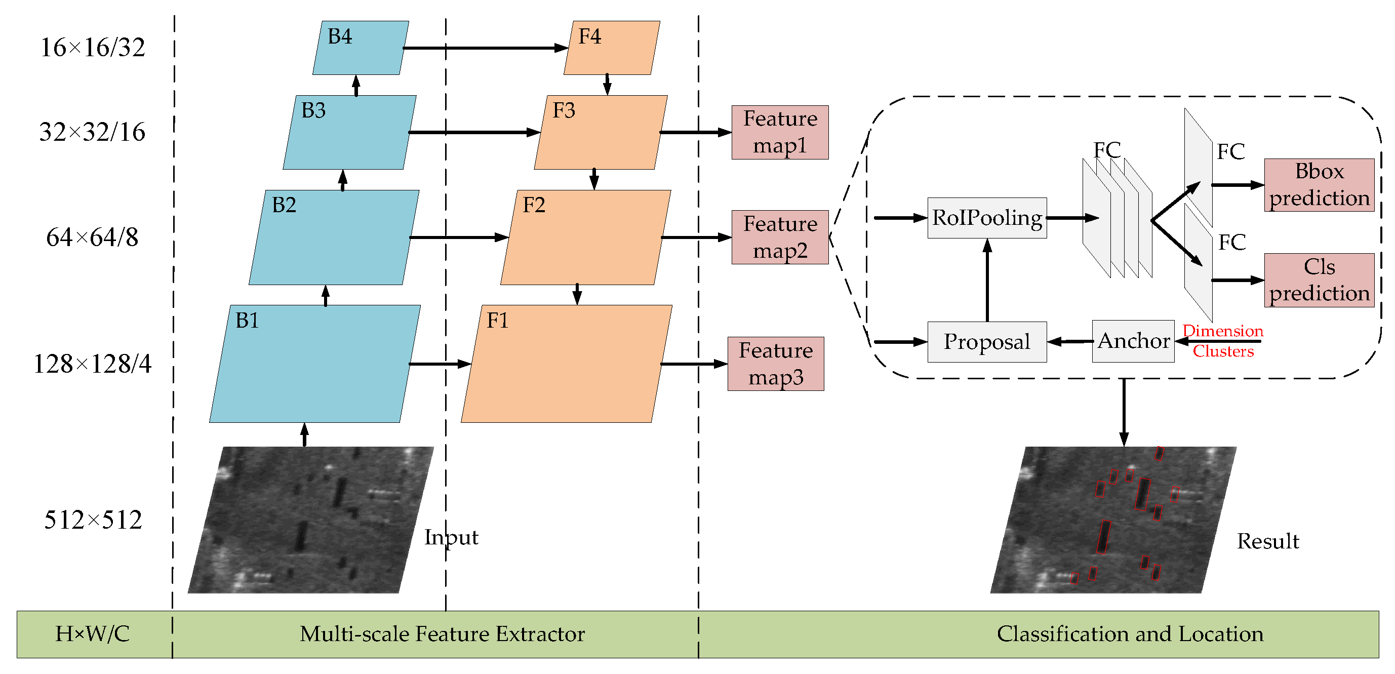
Target detection is the first and the most important step in all TBD-based MTT methods. It significantly determines the tracking performance for multiple targets. Currently, CNN has been widely used for target detection owing to its excellent performance. There are several prevalent CNN-based target detection methods such as Faster-RCNN [18], YOLO [19], and SSD [20]. Among these methods, Faster-RCNN has higher detection performance in optical images since it is a two-stage target detection method that first generates proposals and then uses them for fine target classification and location. Thus, we take it as the basic detection method. To further improve detection accuracy for shadows of moving targets, we modify its feature extractor while applying dimension clusters [21] to obtain anchors. The detailed architecture of multi-scale Faster-RCNN is shown in Figure 3.

2.1.1. Multi-Scale Feature Extractor

For a CNN-based detector, the feature extractor has a great influence on the final detection performance [22,23,24]. Moreover, the features of moving target shadows are not as rich as those of objects in an optical image. Hence, the extractor is required to have a strong feature representation capability. We know that large depth increases the representational ability of a network [25]. Nevertheless, the network instead suffers from model degradation, resulting in performance deterioration [26] when the network depth exceeds a threshold. Owing to the residual network, Resnet [26] solves the above problem and obtains a larger network depth by fusing the upper layer features with the results of the convolution operation to generate the next layer. As a result, it has better model performance. Hence, we choose Resnet50, a version of Resnet, as the basic extractor for extracting features. When the strides are 4, 8, 16, and 32, the corresponding feature maps are denoted by B1, B2, B3, and B4, respectively, as shown in Figure 3.
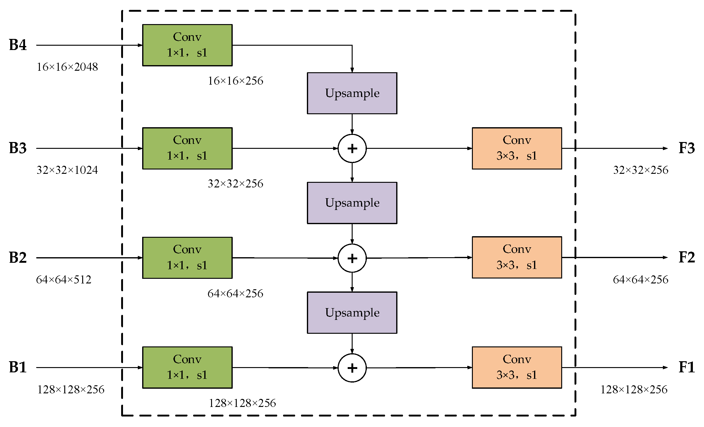
As discussed above, once Resnet50 is well-trained, it can extract higher-level features from the input image by the residual network. However, Resnet50 is a deep top-down structure, which is unfriendly to small objects because the features of small objects will probably be lost in its final output feature maps. Therefore, to eliminate the possibility of feature loss, the feature pyramid network (FPN) [27] is introduced to extract the features of moving target shadows (small objects). As shown in Figure 4, taking the generation of F3 as an example, the B4 feature maps are first convolved by 256 1 × 1 convolution kernels and upsampled by nearest-neighbor interpolation. Meanwhile, the B3 feature maps are convolved by 256 1 × 1 convolution kernels as well. Then, the upsampled feature maps are added with the convolved feature maps. Finally, the added feature maps are convolved by 256 3 × 3 convolution kernels to eliminate the aliasing effect [27] caused by the upsampling operation. As a result, F3 obtains 256 feature maps with a size of 32 × 32 pixels. The same strategy can also be applied to generate F2 and F1. One can see that F1, F2, and F3 all merge features of multiple depths and scales, which extracts more discriminative features while avoiding the above problem.
We constructed the multi-scale feature extractor for shadows of moving targets by the combination of Resnet50 and FPN. It receives an image and outputs feature maps of three different scales. Then we detect and classify targets on these feature maps.

2.1.2. Dimension Clusters

Fast R-CNN is an anchor-based target detection method, i.e., it first requires the generation of proposals for subsequent target classification and location. In Faster-RCNN, the proposals are acquired by regressing anchors designed by hand. However, the manual design approach cannot guarantee that the anchors are well-fitted to the dataset. If the designed anchors deviate excessively from the targets in the dataset, it will affect the regression speed for obtaining proposals. Worse still, Faster-RCNN cannot obtain better network weights because of the bad proposals in the training process, which will lead to reducing its detection performance. Hence, to acquire better anchors, we run the unsupervised learning method, K-means [28,29,30] clustering, on the bounding box of the targets to automatically generate a set of anchors that are better fitted to the dataset. This means that we provide a better prior to the network at the beginning of the training process. Thus, it is easier for the network to obtain better network weights.
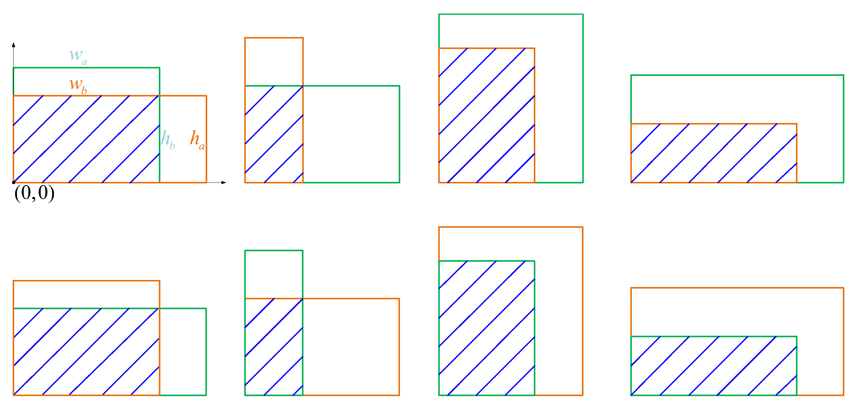
We run K-means generating the anchors. If we use the Euclidean distance for our distance metric directly, large boxes will generate greater errors than smaller boxes in the clustering results. Actually, finding the prior that can obtain good IOU scores is what we really desire. Thus, we use IOU as the distance metric. As shown in Figure 5, suppose that the size of the anchor is w a , h a and the size of the box is w b , h b ; the IOU would thus be defined as:
I O U b o x , a n c h o r = min w a , w b × min h a , h b w a h a + w b h b min w a , w b × min h a , h b
where min denotes an operator that takes the minimum value and max denotes an operator that takes the maximum value.
It is obvious that the IOU score is between 0 and 1. The more similar the anchor and the bounding box are, the higher the IOU score will be. We expect the opposite result. Thus, for our distance metric, we use:
d b o x , a n c h o r = 1 I O U b o x , a n c h o r
From the above equation, when the box and the anchor overlap completely, that is, I O U = 1 , the distance between them is 0.
Given a dataset, suppose that the number of target classes is M, and the number of bounding boxes for each target class is N m , where m 1 , 2 , , M . Let K denote the number of clusters in K-means. We first randomly select K bounding boxes as the initial anchors. Then, we allocate each bounding box to its closest anchor cluster based on the IOU metric. Finally, we calculate the mean of the width and height of all bounding boxes in each cluster to update the anchors. The last two steps of the above process are carried out until the anchors remain unchanged. To make the clustering process easier to read, it is shown in Algorithm 1 below.

2.2. SiamNet

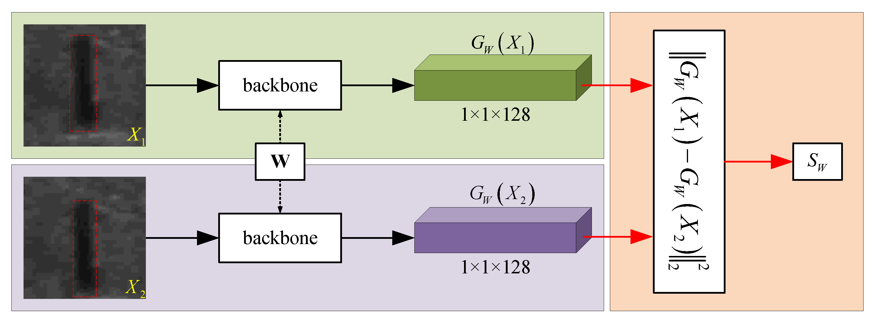
After finishing the detection of the moving target shadows in the search frame, data association, i.e., matching the observations with the moving targets in the template frame, is required for subsequent target tracking. To reduce the matching errors caused by the characteristics of the shadows of moving targets, SiamNet, based on the Siamese network [31], is designed, which compares the similarities between the features of the moving target and the features of the observations to achieve data association. The architecture of SiamNet is shown in Figure 6. It consists of the backbone with the shared parameter W and the cost module. In SiamNet, the backbone maps the inputs into new dimensional space to make similar input vectors to nearby points and dissimilar vectors to distant points. Then, the cost module evaluates the similarity of the outputs from the backbone.
Algorithm 1 Dimension Clusters in the dataset
Input:  The error threshold ε and the set P of bounding boxes of all targets in the dataset.
P = p ( m 1 ) M + n = w m , n , h m , n n = 1 , 2 , , N m , m = 1 , 2 , , M
Begin
1. Initialize: Let t = 0 and select randomly K boxes as the initial anchors Q t .
Q t = q k = p ( m k 1 ) M + n k n k = r a n d ( 1 , N m k ) , m k = r a n d ( 1 , M ) , k = 1 , 2 , , K
2. IOU calculation: Calculate the IOU between each box and each anchor to generate distance matrix D .
for  i = 1 to m M N m  do
    for  i = 1 to m M N m  do
       D p i , q j = 1 I O U p i , q j
    end for
end for
3. Boxes allocation: Allocate each bounding box to its closest anchor and generate the set C of K clusters.
C = c k = p i i f D p i , q k i s min D p i , Q t , i = 1 , 2 , , m M N m , k = 1 , 2 , , K
4. Anchors updating: Let t = t + 1 , and calculate the mean of the width and height of all boxes in each cluster and update the anchors Q t .
Q t = q k = m e a n ( c k ) , k = 1 , 2 , , K
 Determine whether Q t Q t 1 1 ε . If yes, the algorithm ends; otherwise, jump to Step 2.
End
Output:  anchors Q t

2.2.1. Backbone

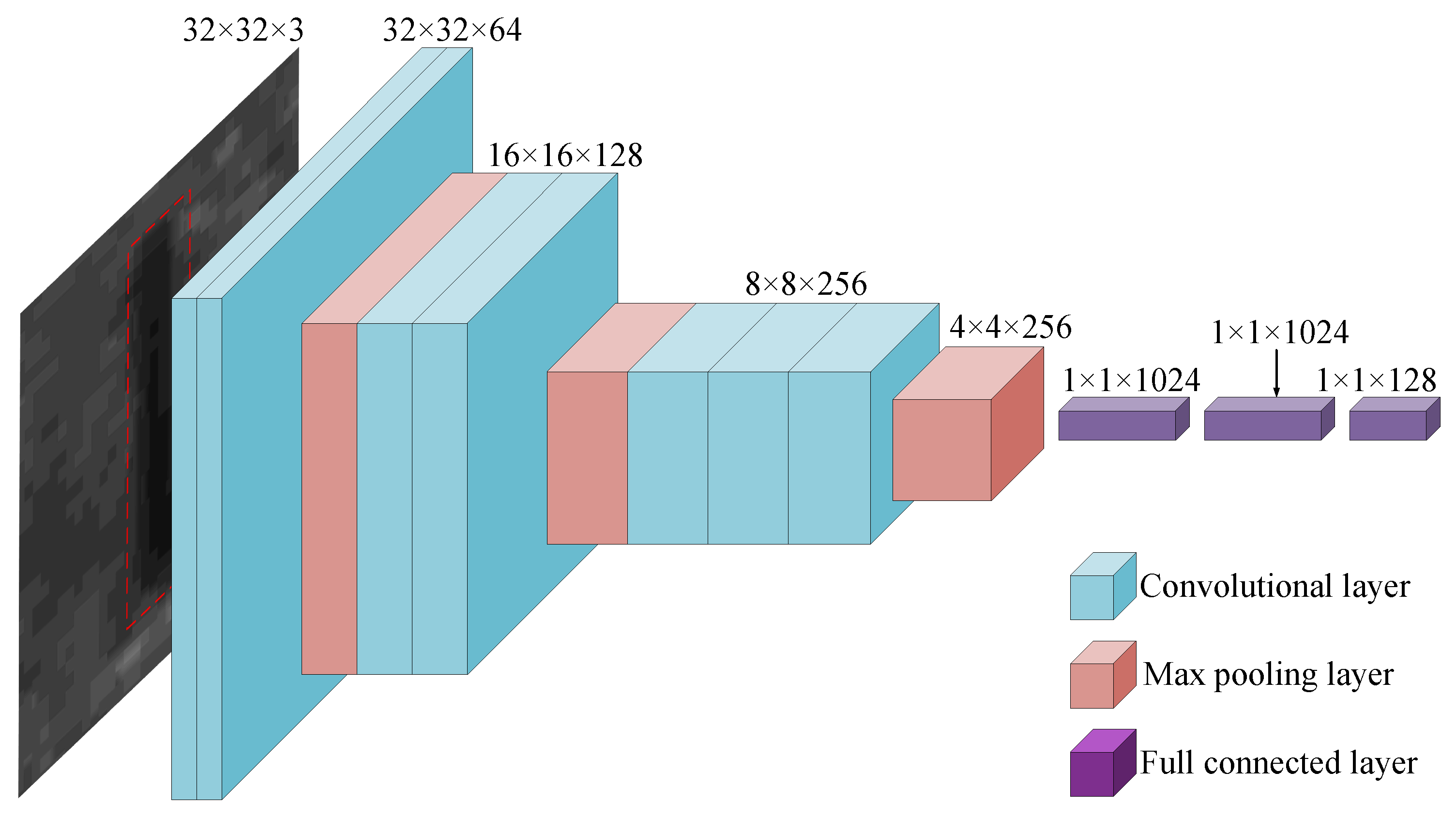
There are many excellent feature extraction networks for optical images, such as Alexnet [13], VGGnet [32], and Resnet [26]. Due to the small size of the moving target shadow, features of the shadow will be lost caused by the large depth of the network. Thus, VGG16 is chosen and modified as the backbone because of its small network depth but powerful performance.
The diagram of the structure of the backbone is shown in Figure 7. Compared to VGG16, our backbone only uses the former seven convolutional layers and the former pooling layers of VGG16. The stride of VGG16 is 32, but the size of the moving target shadow is smaller than 32 × 32 pixels. This means that the moving target shadow does not occupy even a pixel on the final feature maps of VGG16, which prevents VGG16 from extracting the features of the moving target shadows correctly. However, the total stride of our backbone is 8, which guarantees that the above situation will not happen and works for shadows of moving targets. Although the network structure of the backbone is simplified, it still satisfies the current task since the number of targets in our dataset is not as much as that of an optical dataset such as ImageNet.
The network parameters of the backbone are shown in Table 1. “Type” denotes types of different network layers including convolutional layer (“Conv”), max pooling layer (“Pool”), and fully connected layer (“FC”). The “size”, “number”, and “stride” are the kernel parameters in different layers. “Output” is the size of the output feature maps. Layer 0 to layer 10 of the backbone are identical to the structure of VGG16. When SiamNet is used, the backbone first receives an image with the size of 32 × 32 pixels and then outputs a vector with the size of 128 × 1 × 1 . The vector will be used by the cost module for similarity computation.

2.2.2. Contrastive Loss Function

As shown in Figure 7, let X 1 and X 2 denote a pair of patches from the moving target and the observation (a sample). Let Y be a binary label of the pair of images. Y = 0 if the patches X 1 and X 2 are similar, that is, if the observation belongs to the moving target, and Y = 1 if they are deemed dissimilar, that is, the observation does not belong to the moving target. Let G W X 1 and G W X 1 be the outputs of the backbone that are generated by mapping the pair of patches X 1 and X 2 where W is the shared parameter to be learned. Then, the similarity between X 1 and X 2 is transformed into the similarity between G W X 1 and G W X 1 , and we use a scalar “energy function” to measure the similarity between X 1 and X 2 [33]. It is defined as:
S W X 1 , X 2 = G W X 1 G W X 2 2 2
where 2 2 is the Euclidean distance. Then, the most general form of the loss function is
L W = i = 1 N L W , Y , X 1 , X 2 i
L W , Y , X 1 , X 2 i = 1 Y L T S W X 1 , X 2 i + Y L F S W X 1 , X 2 i
where Y , X 1 , X 2 i is the composition of the i-th pair of patches and the label Y, L T is the partial loss function for a similar sample, L F is the partial loss function for a dissimilar sample, and N is the number of training pairs.
Obviously, L T and L F must be designed such that the value of S W for similar samples should be decreased and the value of S W for dissimilar samples should be increased. Moreover, the parameter W is optimized by minimizing L [34].
Thus, the loss function is exactly designed as
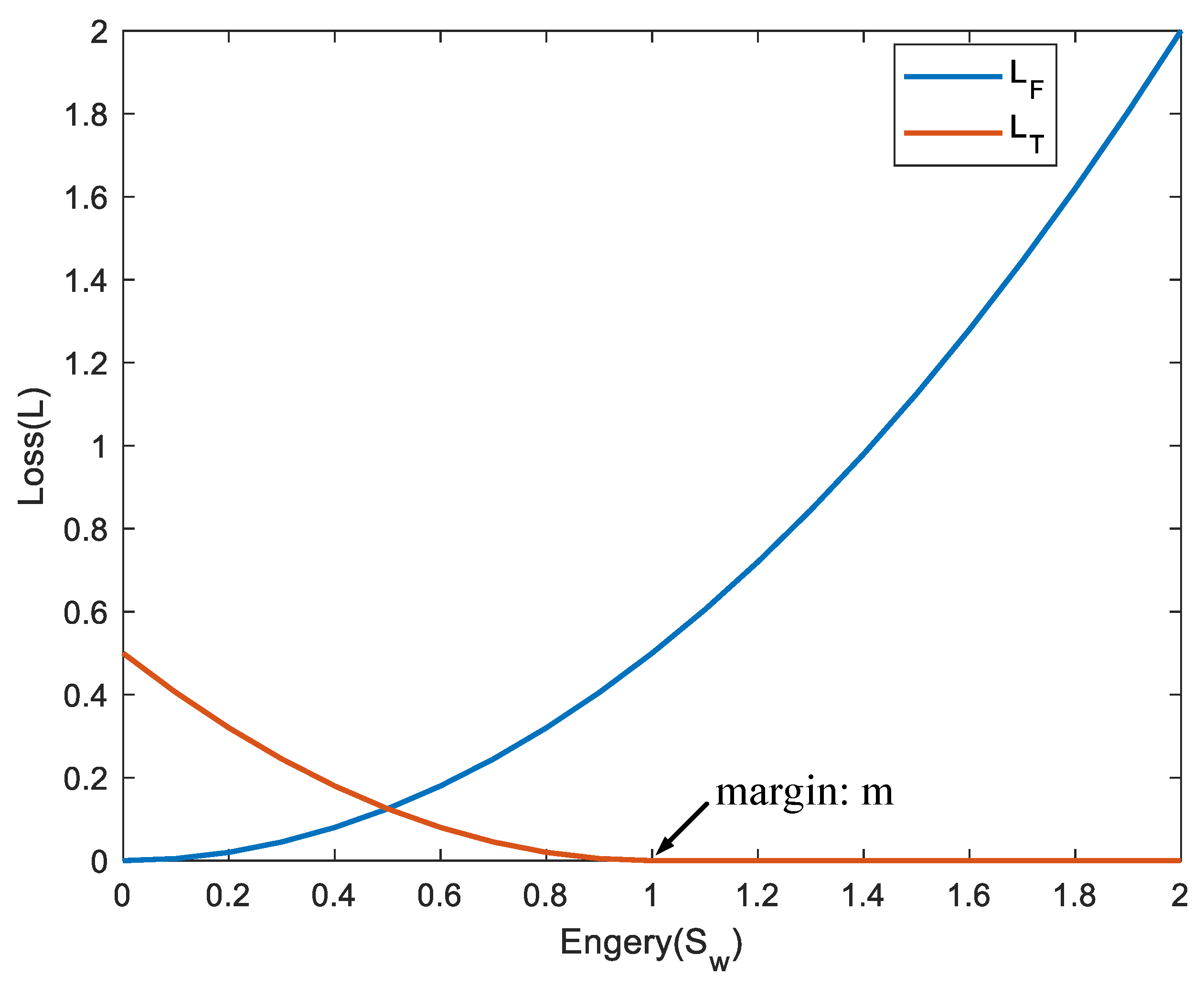
L W , Y , X 1 , X 2 i = 1 Y 1 2 S W X 1 , X 2 i 2 + Y 1 2 max 0 , m S W X 1 , X 2 i 2
where m > 0 is a margin that is defined as a radius around G W X . As shown in Figure 8, the dissimilar samples only work for the loss function if their distances are smaller than this radius. Moreover, the part loss function L F is extremely important for optimizing the parameter W. If the loss is only L T , it will yield a result that S W and the loss L could be made zero by setting G W X to a constant, which is not the expected result.
When SiamNet is trained, transfer learning [35,36] is used in our method. Specifically, we first initialize the backbone of our network by using the network weights trained on the ImageNet dataset then continue training the network with our dataset to optimize the network model. Once the similarity between each moving target and each observation is obtained, it can be used by the Hungarian algorithm to match the moving target with the observation, which realizes the data association.

2.3. Tracking Process

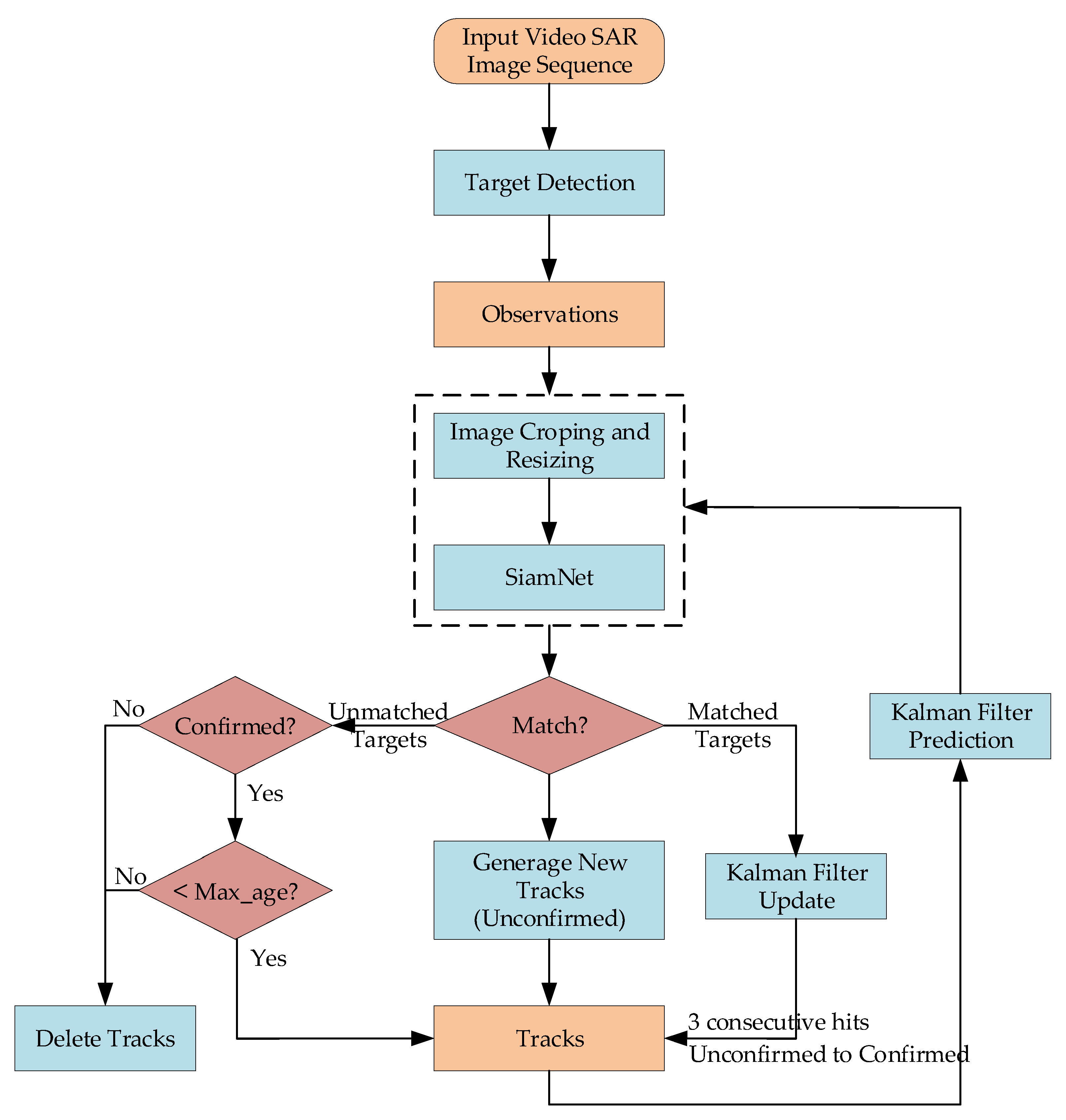
The whole process of Siam-sort for MTT in video SAR is shown in Figure 9. The details are as follows.
Step 1: Target detection using multi-scale Faster-RCNN.
Multi-scale Faster-RCNN is first utilized to detect the shadows of moving targets in the search frame F2. We achieve the detection of the targets, where each detection includes the target’s class, position, size, and confidence, as shown in Figure 10b. To reduce false positives, the confidence threshold is set to remove detections without high confidence, as shown in Figure 10c. Then, the non-maximum suppression (NMS) [37] is applied to eliminate the possibility that a target has more than one detection, as shown in Figure 10d. Finally, we convert the remaining detections into observations. If the search frame is the first frame, a track is generated for each observation, and the observation is recorded in the track. We set the status of each track to be unconfirmed and assign an ID to each track.
Step 2: Image cropping and resizing.
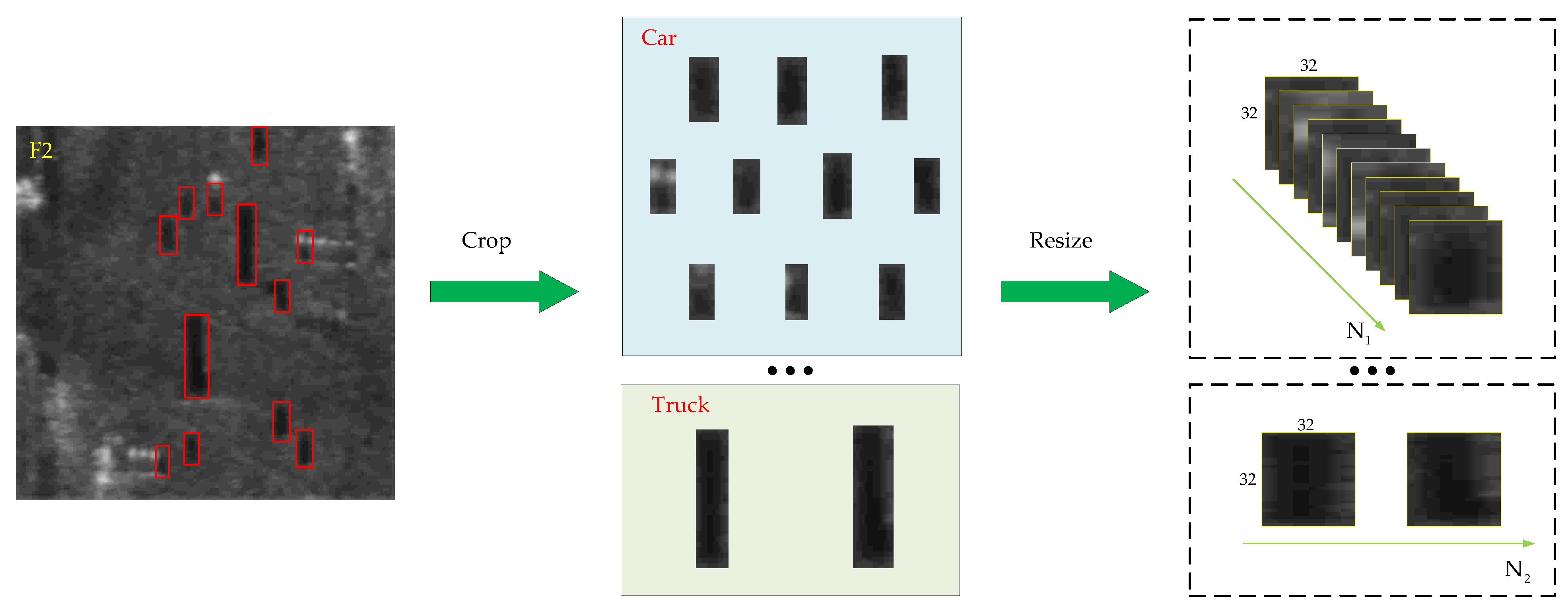
Before using SiamNet, some preprocessing operations are performed. As shown in Figure 11, the image patches of the observations are first cropped out in the search frame, and they are grouped according to the classes of the observations. Then, all the patches are uniformly resized to the size of 32 × 32 pixels to ensure the fully connected layers in SiamNet work properly. In the same way, the image patches of the moving targets in template frame F1 are cropped out and resized. As a result, the image patches of the observations and the image patches of the moving targets are obtained and resized to a uniform size.
Step 3: Data association based on SiamNet.
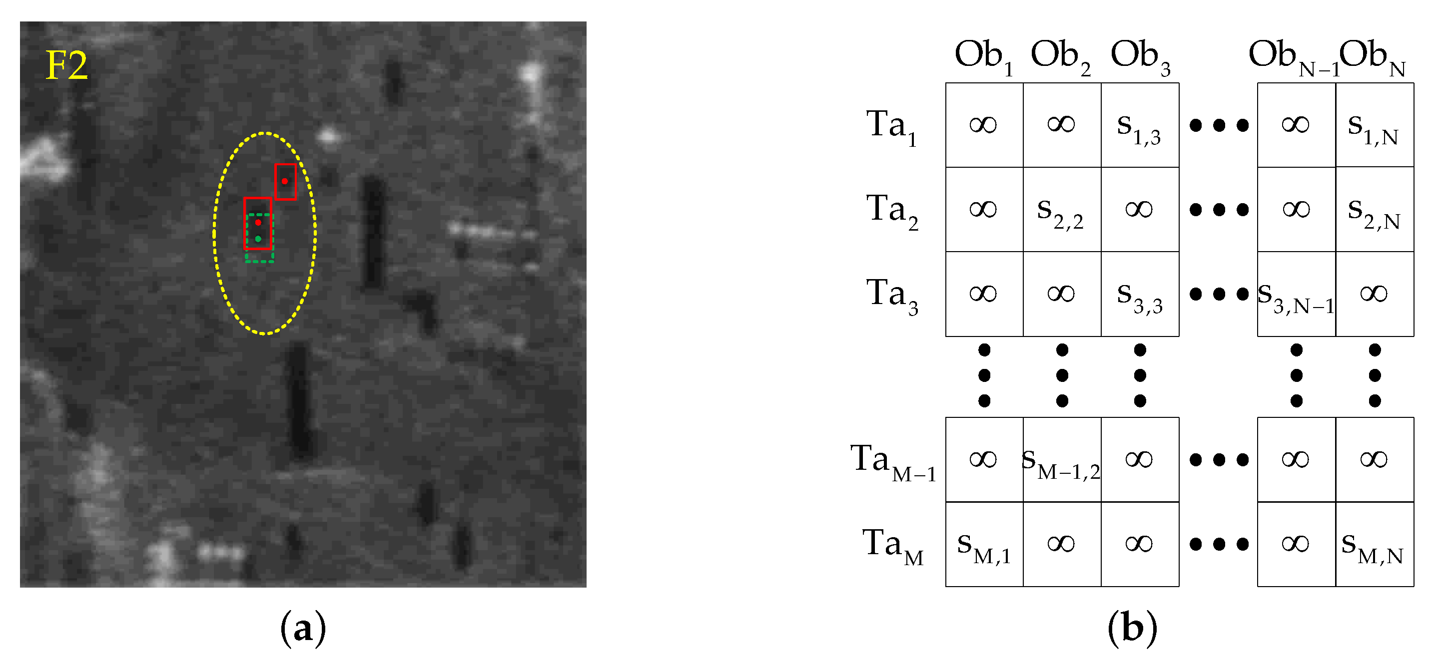
First, the position and the dimension of each target whose track’s status is confirmed are predicted in search frame F2 by using a Kalman filter. Then we calculate the Mahalanobis distance between each target’s predicted position and the position of the observations that have the same class as the target. We set a threshold that determines if the observation is regarded as a possible observation for this target if the Mahalanobis distance between an observation’s position and the predicted position of the target is within the set threshold, as shown in Figure 12a. It is equivalent to a secondary grouping for observations. Then, we calculate the similarities between the target and the possible observations of this target using SiamNet. The similarities of this target with other observations are set to infinity. In this way, we obtain the similarity matrix between all targets and all observations, as shown in Figure 12b. Finally, the Hungarian algorithm is used to match the observations with the targets based on the similarity matrix. For the unmatched observations, they are matched with the true targets that disappear in the template frame F1 but whose tracks’ status is confirmed.
As a result, there are three possible matched results, i.e., unmatched observations, unmatched targets, and matched targets. For unmatched observations, a new track with a new ID is generated for each unmatched observation, and the unmatched observation is recorded in the track. Meanwhile, the status of each new track is set to unconfirmed. For unmatched targets, their tracks are updated by using their predicted positions and dimensions only if their tracks’ status is confirmed and their missing time is shorter than the threshold Max_age. For matched targets, their tracks are updated with their corresponding observations while the patches of the observations are recorded in their tracks (see Step 4).
Step 4: Target tracking using a Kalman filter
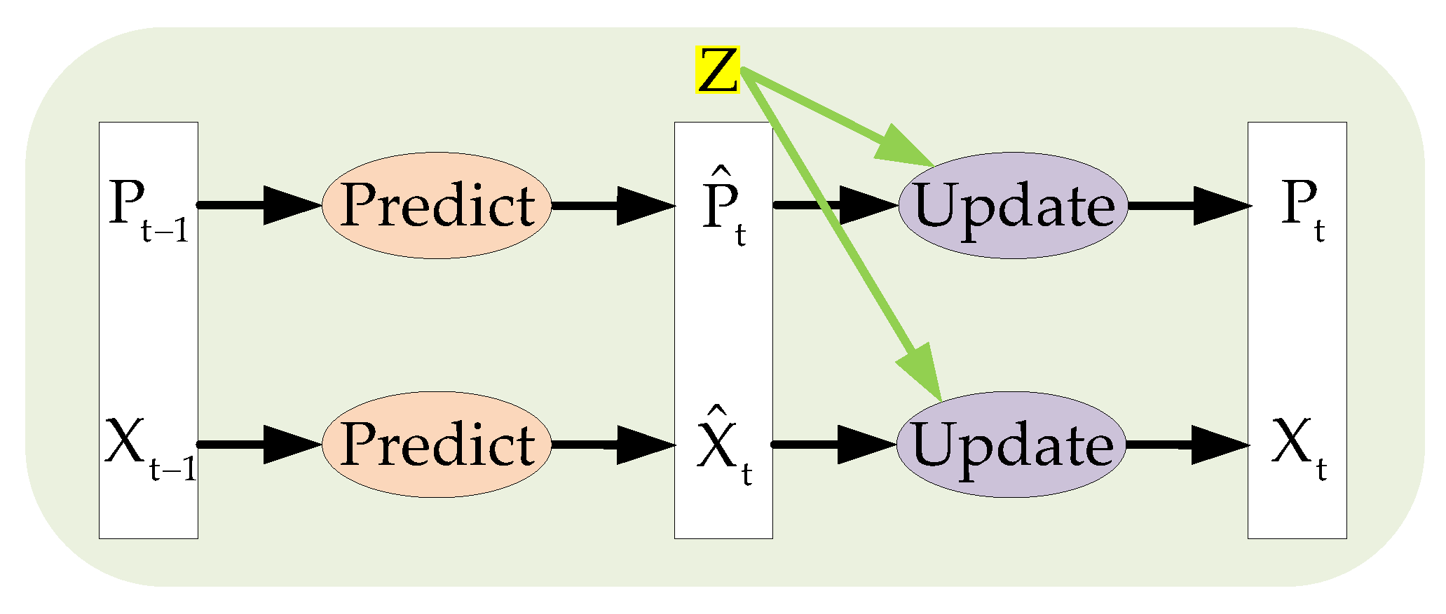
Take a target and its matched observation as an example. Let X t 1 and P t 1 denote the status of the target in the template frame and the covariance of the status, respectively, as shown in Figure 13. We obtain the predictions S ^ t and P ^ t in the prediction stage of the Kalman filter. Let Z denotes the observation. The final tracking result X t and its covariance P t are obtained in the update stage of Kalman filter, and the tracking result is recorded in the target’s track. It is noted that the target is regarded as the true target, and its track’s status is changed to confirmed only if it matches an observation in three consecutive frames.

3. Results

All of the experiments were implemented on a personal computer with an Intel Core i7-8700K CPU, 3.40 GHz, and an NVIDIA GTX1080TI graphics card with 12 GB of memory. The software experiment environment was Windows 10, python 3.7, and PyTorch 1.10.2.

3.1. Experimental Data

There are two real video SAR samples. The first dataset contains 1100 frames. The pixel size of each image is 512 × 512. We use the first 220 frames as the test set for detection and tracking. Then, we use the latter 880 frames as the training set for the detection network, and we crop out the targets in these frames to construct the training set for SiamNet. The second dataset contains 899 frames. The pixel size of each image is 657 × 720. We use the first 120 frames as a test set for detection and tracking. In the same way, the remaining frames are used to construct the training set for the detection networks and SiamNet. Furthermore, we apply data augmentation [38] to expand the dataset.

3.2. Evaluation Indicators

3.2.1. Detection Indicators

Siam-sort is a TBD-based method, and its detection performance has a significant impact on the final tracking performance of the MTT. Therefore, we use three evaluation indicators to verify the detection performance [18,19,20]:
  • Average precision @50 (AP@50): The average precision for a target category when the IOU is set to 0.5;
  • Average precision @75 (AP@75): The average precision for a target category when the IOU is set to 0.75;
  • Average precision @[50:95] (AP@[50:95]): The average precision for a target category when the IOU is set from 0.5 to 0.95.

3.2.2. Tracking Indicators

To verify the tracking performance of Siam-sort, seven general evaluation indicators are used in this article [39].
  • Multi-target tracking accuracy (MTTA): The total tracking accuracy for false negatives, false positives, and identity switches;
  • Multi-target tracking precision (MTTP): The total sum of overall tracking precision calculated from bounding box overlap between the label and the detected position;
  • Mostly tracked (MT): Number of ground-truth targets that have the same label for at least 80% of their lifetime;
  • Mostly lost (ML): Number of ground-truth targets that are tracked in a maximum of 20% of their lifetime;
  • Identity switches (IDS): Number of changes in the identity of a ground-truth target;
  • Fragmentation (FM): Number of interrupted tracks due to missing detection;
  • Frame per speed (FPS): The average running time of the tracking algorithm for one frame.

3.3. Results of the First Real Video SAR Dataset

3.3.1. Detection Results

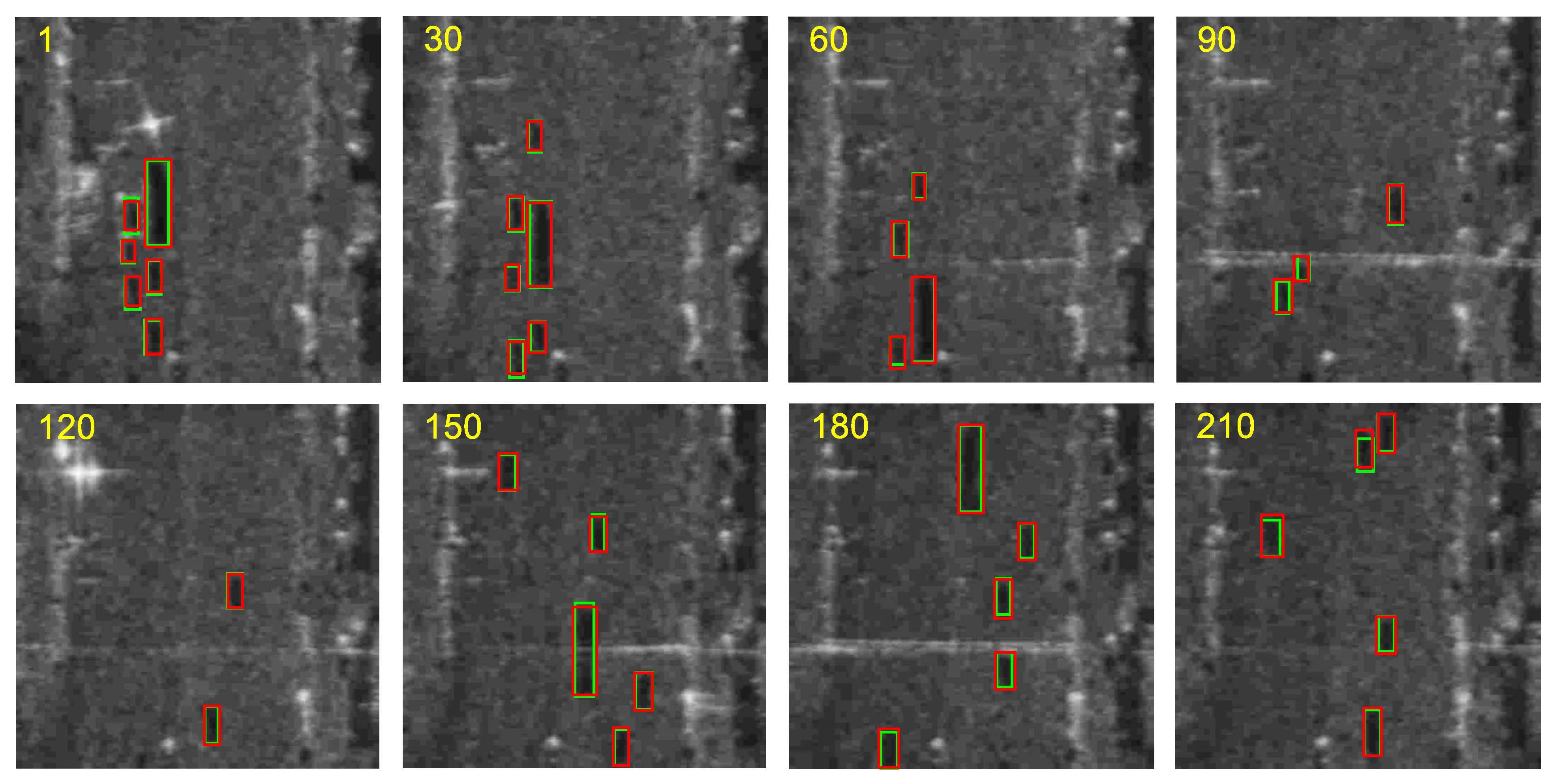
Figure 14 shows the detection results obtained by using multi-scale Faster-RCNN at frame 1, frame 30, frame 60, frame 90, frame 120, frame 150, frame 180, and frame 210. The green boxes denote the ground truths of the moving targets, and the red boxes show the detection results. It can be seen that all the moving targets are detected successfully and the bounding boxes of the detection results almost exactly overlap with those of ground truths. It illustrates the effectiveness of the proposed multi-scale Faster-RCNN for moving target detection in video SAR images.
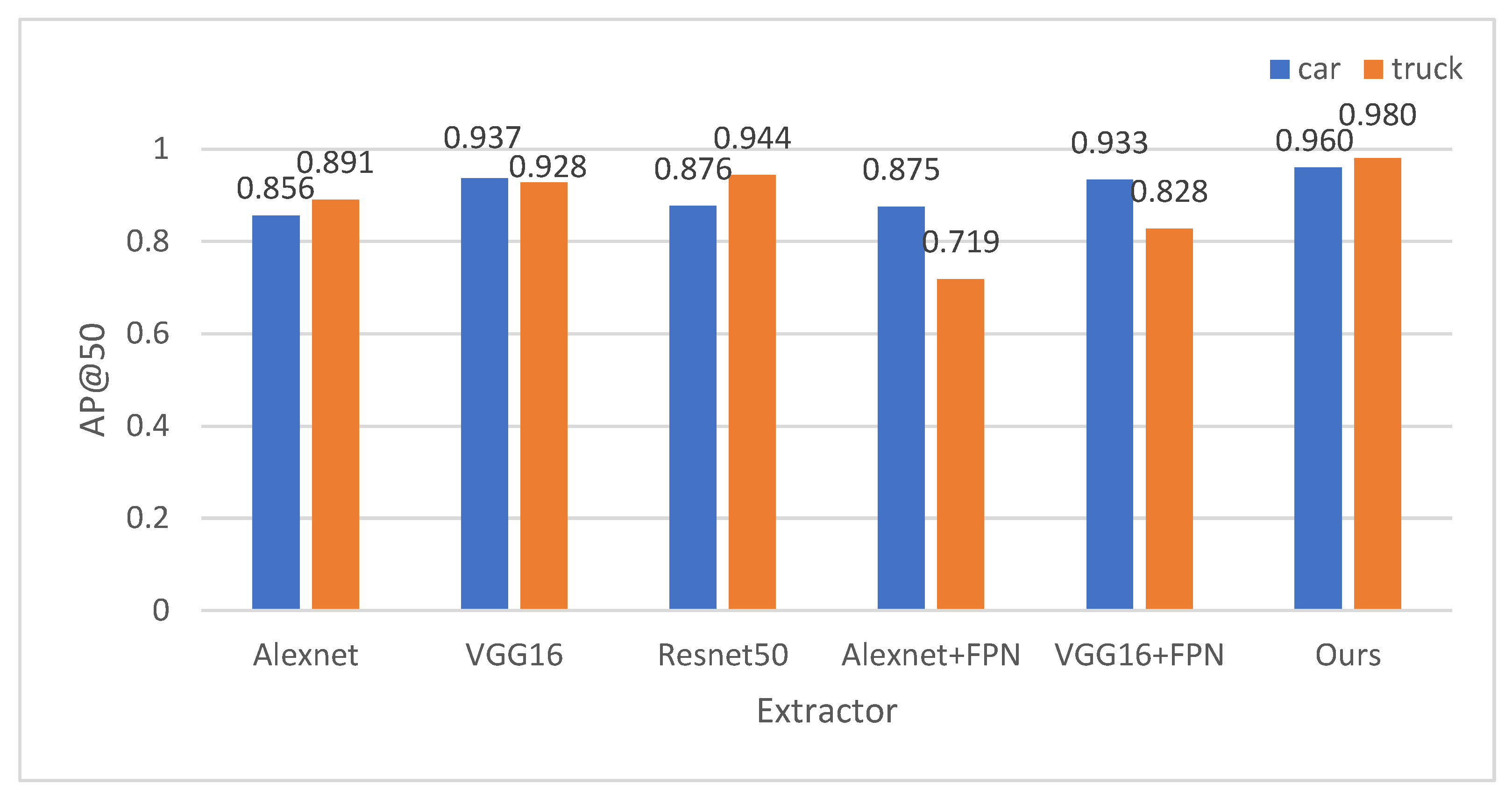
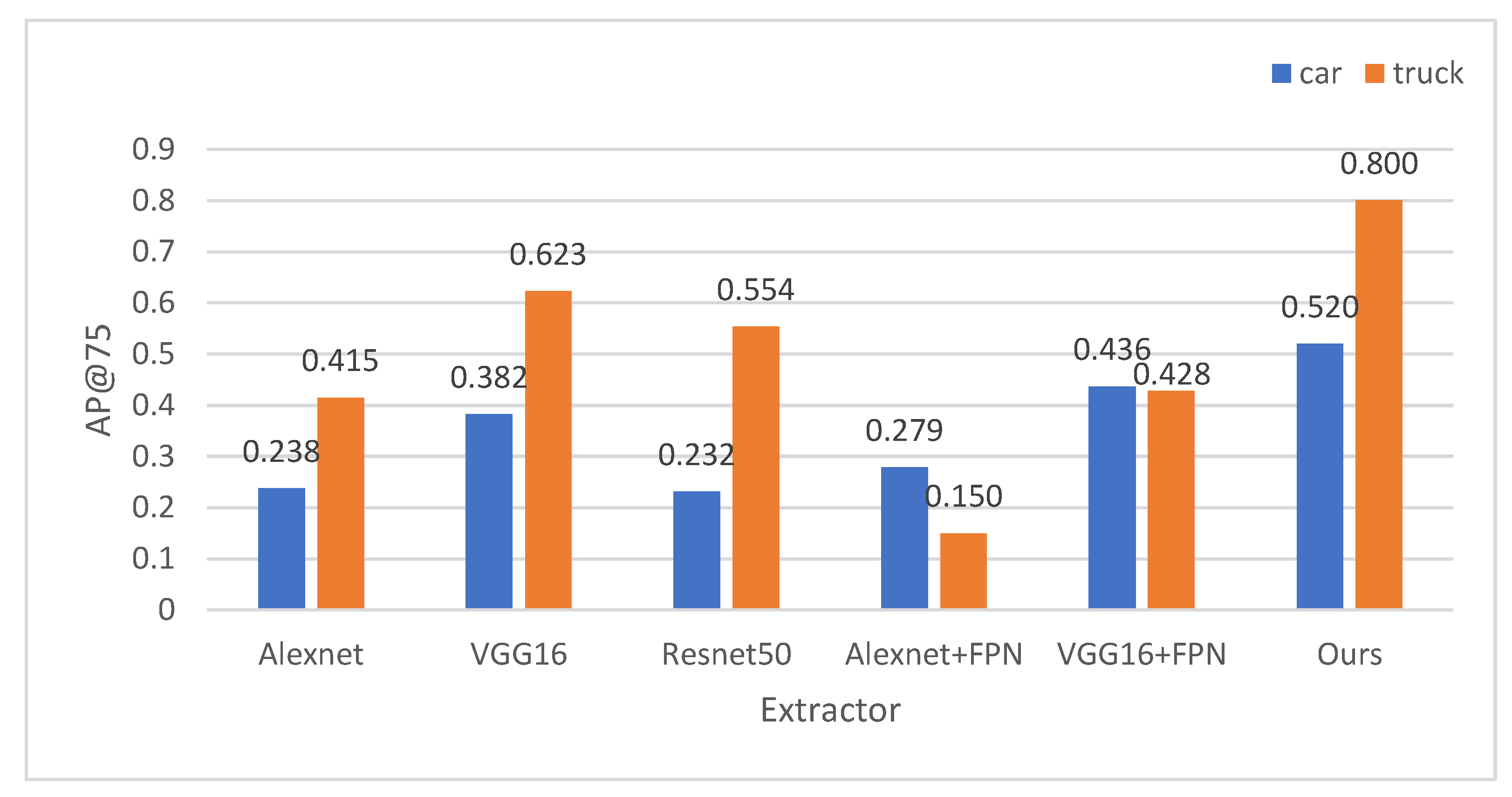
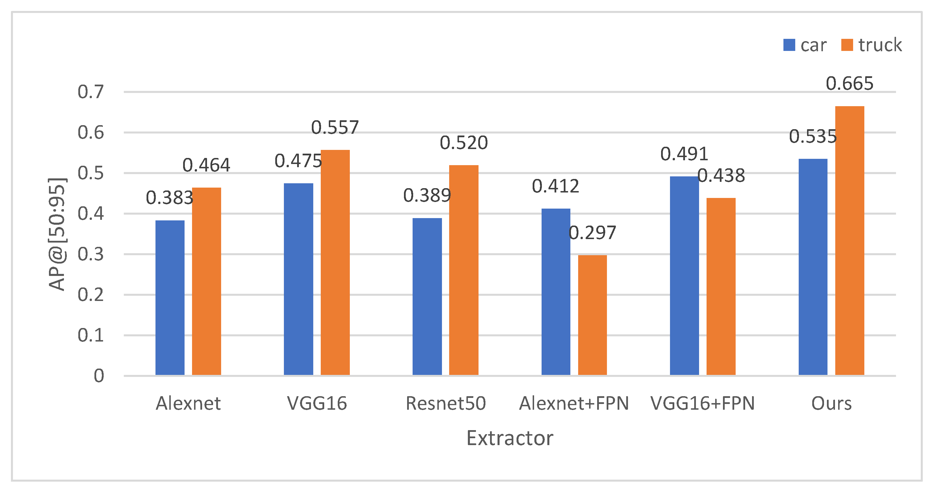
To further validate our method, we compare the proposed detection method with Faster-RCNN using five different extractors including Alexnet, VGG16, Resnet50, Alexnet with FPN, and Vgg16 with FPN. To keep the experiment reasonable, all methods were performed under the same experimental environment and settings. Meanwhile, dimension clusters were applied to all methods. Figure 15, Figure 16 and Figure 17 show the comparison results in different target classes of the proposed detection method with Faster-RCNN using other extractors.
One can see that the proposed detection method improves AP@50 by at least 2.3%, AP@75 by at least 9%, and AP@[50:95] by at least 4.4% in the car class. The improvements are 5.2%, 17.7%, and 10.8%, respectively, in the truck class. These results indicate that the proposed extractor is superior to other extractors so that the proposed detection method has a better detection performance. We find that the scores of Resnet50 are lower than those of Alexnet and VGG16 on the three indicators, which demonstrates the large depth of Resnet50 degrades the feature extraction ability for small targets, resulting in a deterioration in detection performance. Moreover, unlike Resnet50, the lower scores are obtained on the truck class when VGG16 and Alexnet use FPN. The reason for this is that FPN causes each feature map to only detect the targets in a specific size range [40], and the larger targets are only detected using the lower-layer feature maps. However, each feature map of Resnet50 is fused with multi-layer features so that each feature map can work for all targets.
Table 2 shows the mean results for all target classes in the test set. It can be seen that our method has still the highest scores on all indicators, which also verifies the effectiveness of the proposed feature extractor and the superiority of the proposed detection method.

3.3.2. Tracking Results

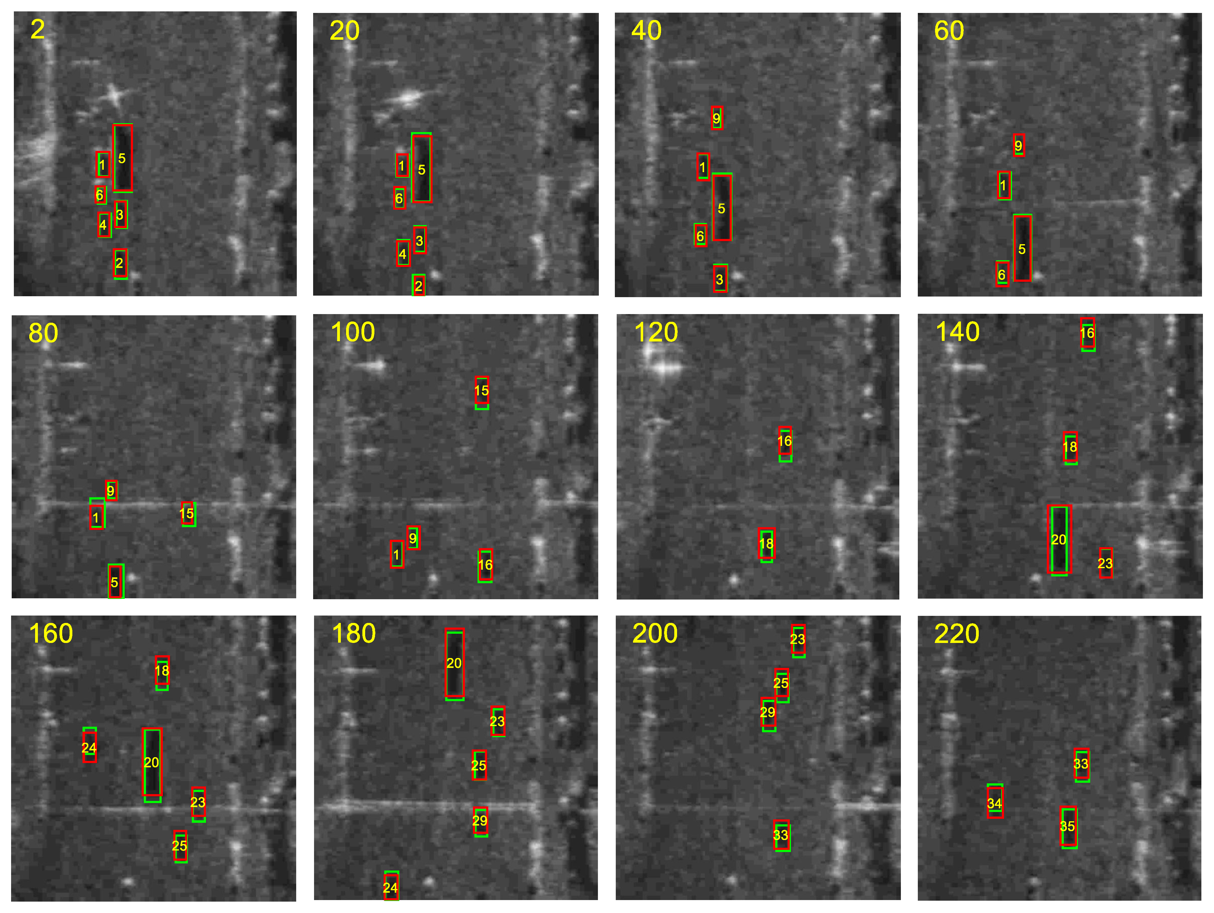
Figure 18 shows the tracking results at frame 1, frame 20, frame 40, frame 60, frame 80, frame 100, frame 120, frame 140, frame 160, frame 180, frame 200, and frame 220. The green boxes denote the ground truths of the moving targets, and the red boxes mean the tracking results. The ID of the target is marked in the center of the red box. It can be seen that all targets are tracked and their IDs remain unchanged at these frames. Meanwhile, the boxes of the tracking results almost exactly overlap with those of ground truths. The above results illustrate the proposed method has high tracking accuracy and tracking precision.
Table 3 shows the statistical tracking results for each target in the test set. ‘MT?’ indicates whether the tracking result of the target is counted in MT, and ‘ML?’ indicates whether the tracking result of the target is counted in ML. One can see that the tracking results for each target belong to MT rather than ML, which illustrates that each target is being tracked for at least 80% of its lifetime. Furthermore, the number of IDS for all targets is 0, even if some of them are tracked discontinuously (FM > 0). This indicates that the ID of each target remains unchanged during its lifetime. The statistical results demonstrate the effectiveness of SiamNet in data association and the robustness of Siam-sort for MTT.
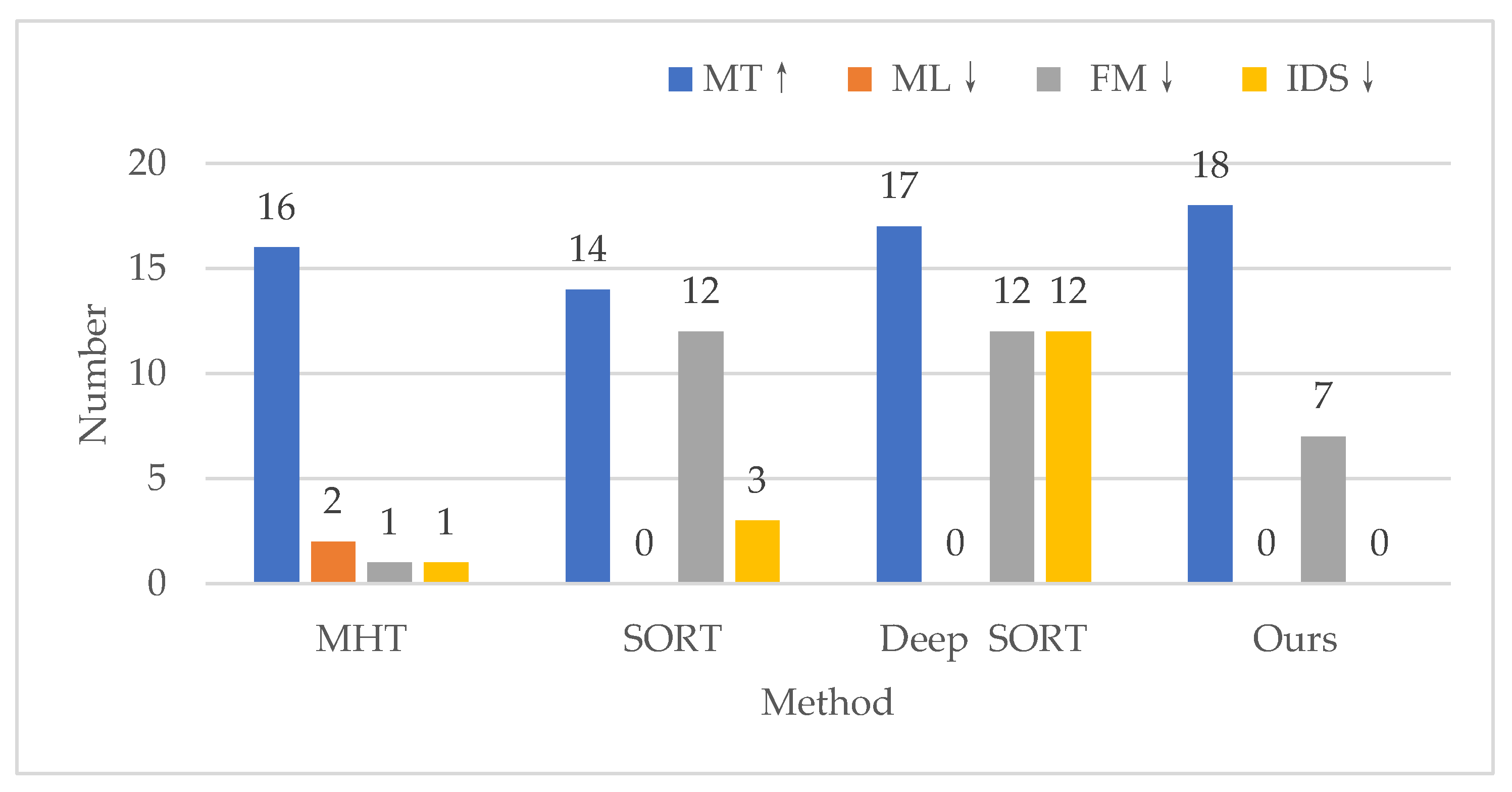
To verify the superiority of Siam-sort, we compare the proposed method with other state-of-art methods, including MHT [41], SORT, and Deep SORT. The comparison results are shown in Figure 19. It can be seen that our method has the highest number of MT targets and the least number of ML targets (18 MT, 0 ML), illustrating that our method achieves tracking for all the targets. Meanwhile, our method has the least number of IDS (0 IDS), which demonstrates that our method has the best performance for data association compared to other methods. We find that the number of FMs of our method is less than that of SORT. The reason for this is the number of FMs is incorrectly counted resulting from the failed tracking for the two targets in the test set by MHT. Without counting the number of FMs for these two targets (target 6 and target 7 in Table 3), the number of FMs of our method is equal to that of MHT. However, our method is ahead of MHT on all other indicators. The above analysis demonstrates that our method outperforms MHT, SORT, and Deep SORT for MTT.
Table 4 shows the comparative results of the four MTT methods on the three overall indicators. We can see that the tracking accuracy of our method is substantially higher than that of SORT and MHT (0.947 MTTA). In addition, the tracking precision of our method is also the highest (0.869 MTTP) compared to other methods. Although our detection method (12.505 FPS) is not the fastest in terms of tracking speed, it still satisfies the practical tracking requirements due to the lower imaging speed of the video SAR system [42]. The details are given in Appendix A.

3.4. Results of the Second Real Video SAR Dataset

To further validate the performance of Siam-sort, we test it on another real video SAR dataset.

3.4.1. Detection Results

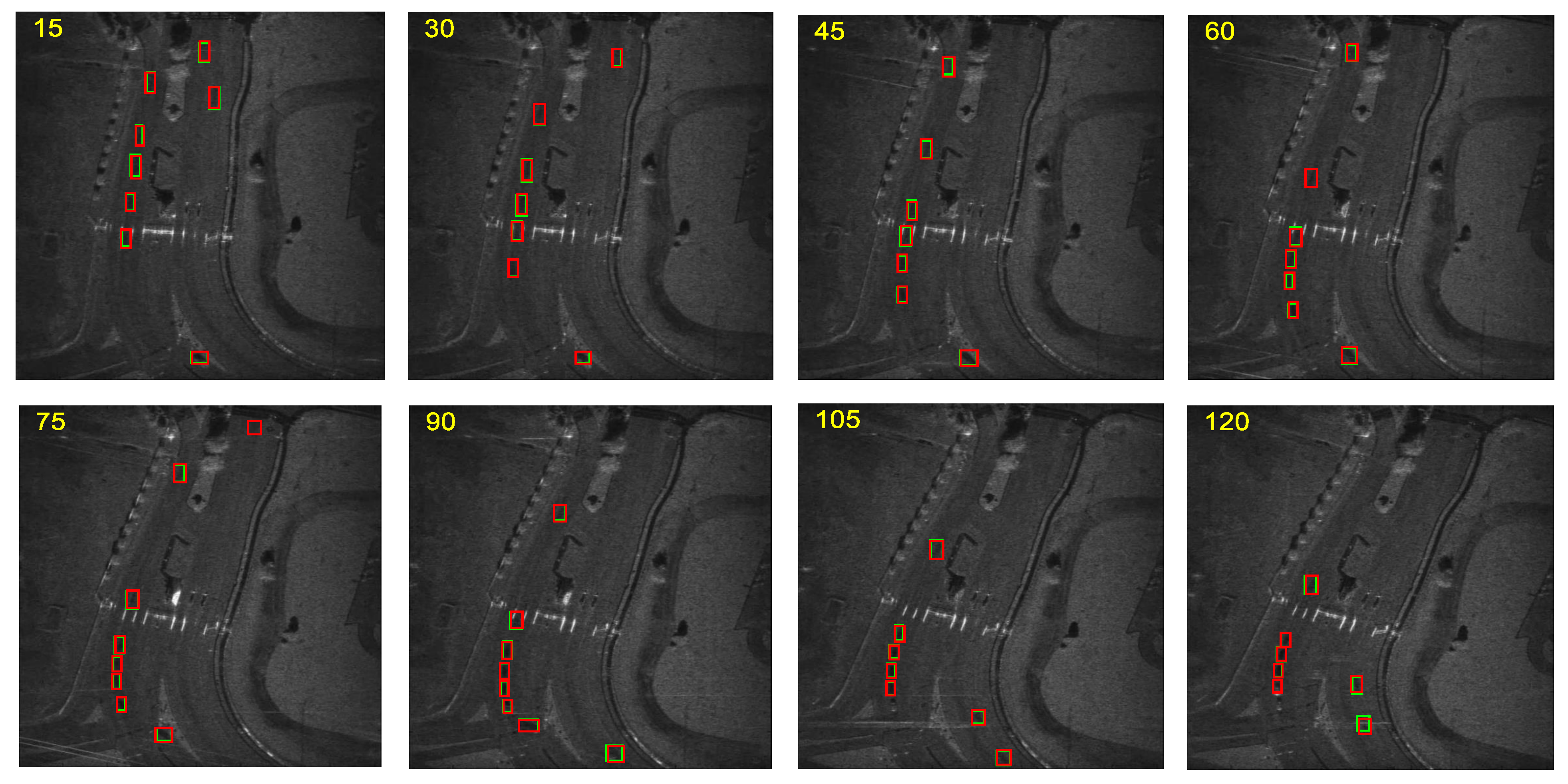
Figure 20 shows the detection results of eight frame images in the second test set. In these frame images, all targets are detected successfully, and their bounding boxes almost overlap with those of the ground truths, which illustrates that the proposed detection method has high detection accuracy and detection precision.
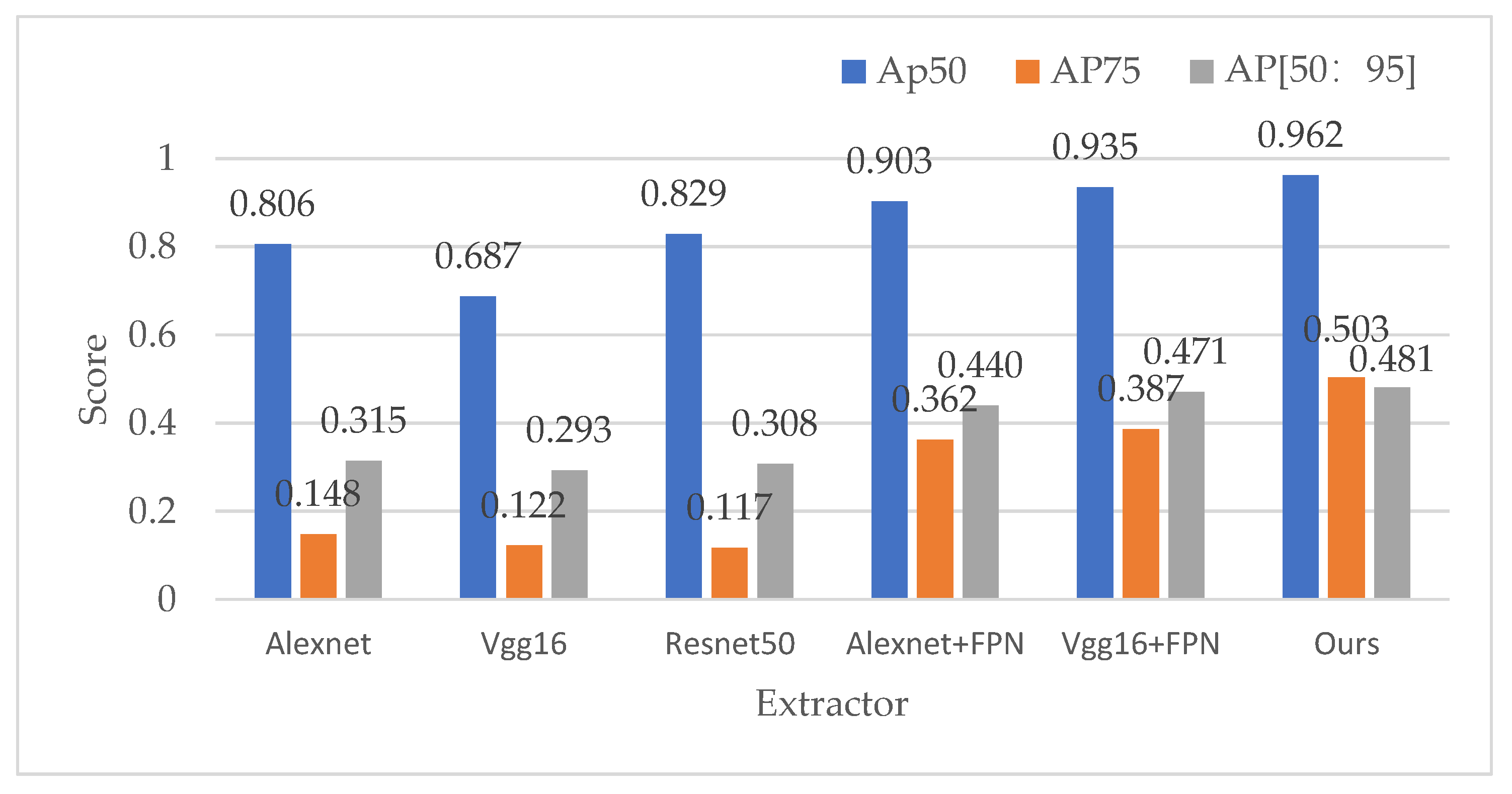
Likewise, we also compare the proposed detection method with Faster-RCNN based on other extractors in the second test set to validate the detection performance of the proposed detection method, as shown in Figure 21. It can be seen that the proposed detection method obtains the highest scores on three indicators compared to the other methods, which demonstrates that our method outperforms other methods. We do not show the mean results for all target classes because the second test set only possesses one target class.

3.4.2. Tracking Results

Figure 22 shows the tracking results of Siam-sort on twelve image frames from the second test set. The green boxes denote the ground truths of the moving targets and the red boxes mean the tracking results. It can be seen that our method still successfully tracks all targets in this test set.
Table 5 shows the statistical tracking results for each target in the second test set. In this table, the tracking results of each target are all counted in the MT category, which indicates that they are all tracked successfully. Moreover, the number of their IDS and FMs are both 0, meaning that they are tracked continuously. Therefore, the proposed method is still effective for MTT in this test set.
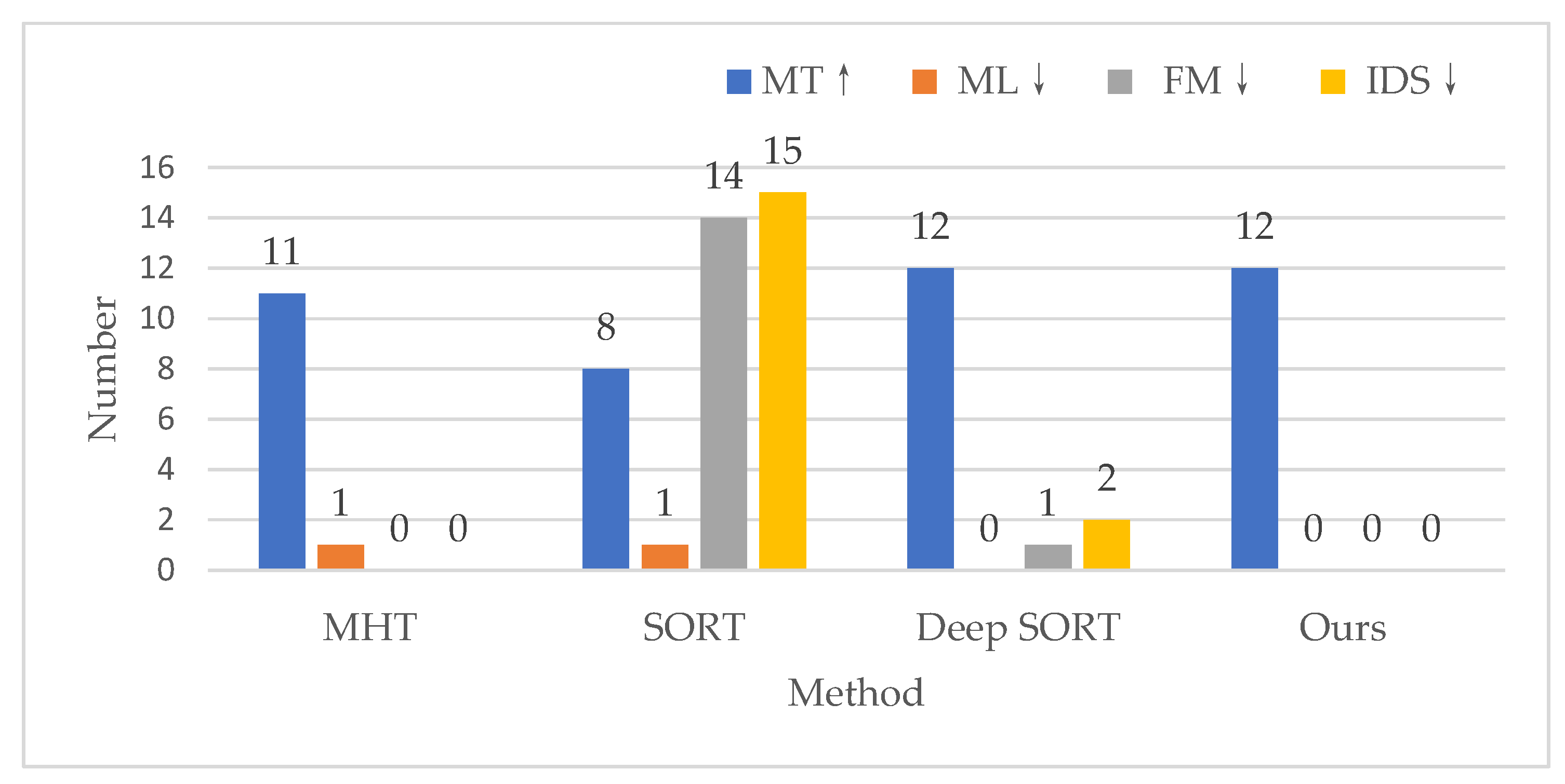
We also compared Siam-sort with other methods. As shown in Figure 23, the numbers of FMs and IDS of the proposed method (0 FM and 0 IDS) are the lowest, while all the targets are successfully tracked (12 MT). We also compare the four methods on three overall indicators, as shown in Table 6. Our method still has the highest tracking accuracy and tracking precision (0.954 MTTA and 0.876 MTTP), which demonstrates that our method outperforms other methods for MTT in video SAR.

4. Discussion

4.1. Choice of K Value in the Dimension Clusters

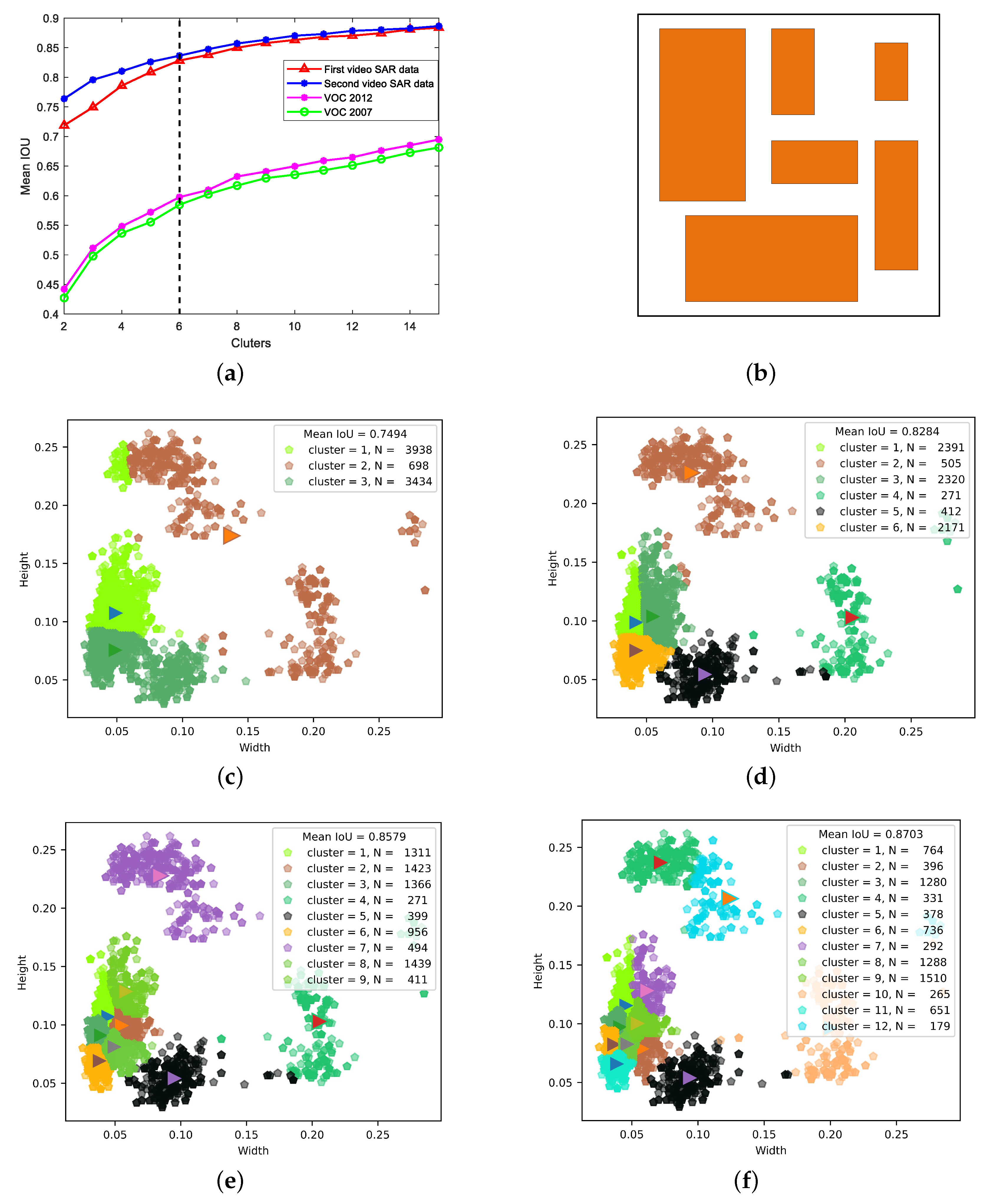
We run k-means clustering with different values of K and plot the variation of the mean IOU. As shown in Figure 24a, the mean IOU score grows as the K value increases. We chose K = 6 as a tradeoff to meet both the high recall and low model complexity. The relative anchors obtained by K-means clustering on the first video SAR dataset are shown in Figure 24b. The shapes of the obtained anchors mostly tend to be tall and thin. Figure 24c–f show the clustering results when different values of K are taken ( K = 3 , 6 , 9 , and 12). Points of different colors belong to different clusters centered on an anchor. We can find that the majority of target sizes tend to be taller, which verifies the accuracy of the clustering results.
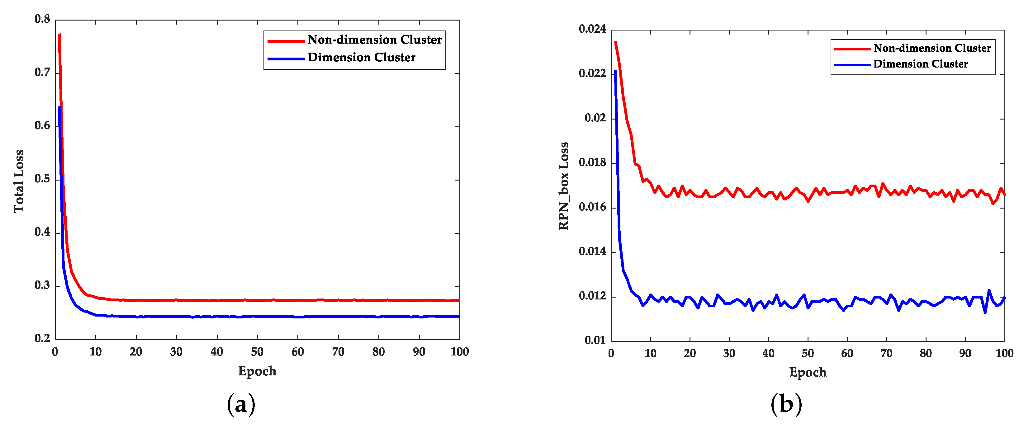
To illustrate the influence of dimension clusters in the training process, we train multi-scale Faster-RCNN with and without using dimension clusters. The number of epochs is set to 100, and the variation in total loss and box loss of RPN with the training epoch is shown in Figure 25. It can be seen that the convergence speed of the box loss of RPN with dimension clusters is significantly faster than that without dimension clusters. Furthermore, both the total loss and the box loss of RPN with dimension clusters converge to smaller values. This indicates that the detection network is allowed to obtain better network weights by using dimension clusters so that it has better detection performance.
Table 7 shows the detection performance of multi-scale Faster-RCNN with and without dimension clusters. Compared to the case without dimension clusters, Faster-RCNN with dimension clusters obtains higher scores on three indicators. It also evidences that dimension clusters allow multi-scale Faster-RCNN to obtain better detection performance.

4.2. Research on Background Occlusion

In real scenes, the shadows of moving targets are quite likely to be obscured, which leads to missed detection. Hence, the MTT method is required to have two capabilities. One is that, when the target is obscured in only one frame, the MTT method must be able to track the target in that frame. The other is that when the target is obscured in consecutive frames but reappears in subsequent frames, the MTT method must be able to re-track the target in subsequent frames. In this article, to track a target in the frame where the target is obscured, Siam-sort takes the prediction result of the Kalman filter as the tracking result. To re-track the target, Siam-sort matches the target in the frames before the target is obscured with the observation in the subsequent frame by using SiamNet (see Step 3 in Section 2.3 for details). As described above, to re-track the target, the target must be retained, i.e., the number of frames in which the target is continuously undetected must less than the threshold Max_age. Therefore, the threshold Max_age should be set to a larger value when the target in the scene is obscured for a longer time.
Figure 26 shows tracking results when the target is obscured in only one frame. It can be seen that target 2 is obscured by background clutter and that it can be tracked again at frame 28. Figure 27 shows the re-tracking results after the target is obscured in consecutive frames. Suppose target 5 is obscured from frame 11 to frame 20 and we artificially hide the observations of target 5 in those frames. When the threshold Max_age is set to 9, the target’s ID switches, meaning that the target failed to be re-tracked, as shown in Figure 26c. In addition, the target’s ID remains unchanged, meaning that the target is re-tracked successfully when the threshold Max_age is 11, as shown in Figure 26d.

4.3. Ablation Experiment

We test the key components (multi-scale Faster-RCNN and SiamNet) to see their impact on the tracking performance. Specifically, we compared the two variants (baseline + multi-scale Faster-RCNN and baseline + multi-scale Faster-RCNN + SiamNet) with the baseline, as shown in Table 8. In the baseline, VGG16 is used to detect moving targets, and HOG features [43] are used for data association. Comparing the first row with the second row, multi-scale Faster-RCNN increases the number of MT targets by 3 and reduces the number of FMs by 6. Comparing the third row with the second row, the number of IDS reduces sharply and becomes 0. Comparing the third row with the first row, multi-scale Faster-RCNN and SiamNet improve MTTA by 7% and MTTP by 3.8%. Based on the experimental results above, multi-scale Faster-RCNN and SiamNet indeed greatly contribute to improving tracking accuracy and tracking precision.

5. Conclusions

In this article, to achieve MTT in video SAR, we proposed a novel TBD-based method, Siam-sort. Specifically, we first proposed a multi-scale Faster-RCNN to improve the detection accuracy for shadows of moving targets. Then, to further improve detection performance, we applied dimension clusters to give multi-scale Faster-RCNN a better prior in the training process. Furthermore, we proposed SiamNet, which used the similarities between features of target shadows and features of observations to achieve data association. In two real video SAR data, Siam-sort acquired the best grades on all indicators, which demonstrated that our method outperformed MHT, SORT, and Deep SORT. Additionally, the grades on all indicators were improved in the ablation experiment, which verified the effectiveness of a multi-scale Faster-RCNN and SiamNet.

Author Contributions

H.F. and G.L. designed the experiment and analyzed the data; H.F. and Y.L. performed the experiments; H.F. wrote the paper, Y.L. and C.Z. revised the technical errors and grammar of the paper. All authors have read and agreed to the published version of the manuscript.

Funding

This work was supported in part by the Nature Science Foundation of China (NSFC) under Grants 61931016 and 62071344, in part by the National Natural Science Foundation of China under Grant No.62001352, and by the Open Foundation of CETC Key Laboratory of Data Link Technology under Grant CLDL-20202412.

Data Availability Statement

Not applicable.

Acknowledgments

The authors thank all reviewers for their comments toward improving our manuscript, as well as the Sandia National Laboratory of the United States for providing SAR images.

Conflicts of Interest

The authors declare no conflict of interest.

Appendix A

The major task of the video SAR system is to achieve continuous observation of the area of interest in all-day and all-weather conditions; thus, it usually adopts the spotlight imaging mode with circular trajectory. According to the SAR imaging theory in the above mode, the azimuth resolution is related to the azimuth accumulation angle:
ρ a = k λ 2 θ s
where ρ a denotes the azimuth resolution, λ denotes the radar wavelength, θ s denotes the azimuth accumulation angle, and k is set to 1.2 based on experience. Thus, the azimuth accumulation angle θ s can be obtained as follows:
θ s = k λ 2 ρ a
According to [42], the synthetic aperture time for generating one SAR image can be expressed as:
T a = θ s r a v = k λ r a 2 ρ a v
where v denotes the velocity of the video SAR and r a denotes the distance between the video SAR and the scene center. Supposing the imaging time is ignored, the frame rate of video SAR is inversely proportional to the synthetic aperture time, that is,
F s = 1 T s = 2 ρ a v k r a c f c
where f c is the carrier frequency.
Firstly, to achieve accurate identification of targets in the observation area, the imaging resolution of video SARA is required to reach 0.2 m, that is, ρ a 0.2 m. Secondly, to increase the frame rate, the carrier frequency of the video SAR should be increased maximally. Nevertheless, due to the severe atmospheric attenuation of the radar signal with high carrier frequency, only 94 GHz, 220 GHz, and 340 GHz with lower atmospheric attenuation can be selected as the carrier frequency, and the operation range of video SAR is limited. Furthermore, the velocity of video SAR is normally below 150 m/s. Suppose that all variables reach their extreme values, that is, ρ a = 0.2 m, v = 150 m/s, and f c = 340 GHz. r a is reasonably set to 5 km. Taking the values of all variables into (A4), the maximum frame rate we obtain is 11.333 Hz. If the imaging time is considered, the maximum frame rate will be substantially lower than 11.333 Hz. Based on the above analysis, the real-time performance of the proposed method satisfies the practical multi-target tracking requirements.

References

  1. Qin, S.; Ding, J.; Wen, L.; Jiang, M. Joint track-before-detect algorithm for high-maneuvering target indication in video SAR. IEEE J. Sel. Top. Appl. Earth Obs. Remote Sens. 2021, 14, 8236–8248. [Google Scholar] [CrossRef]
  2. Raynal, A.M.; Bickel, D.L.; Doerry, A.W. Stationary and moving target shadow characteristics in synthetic aperture radar. In Radar Sensor Technology XVIII; SPIE: Bellingham, WA, USA, 2014; pp. 413–427. [Google Scholar]
  3. Miller, J.; Bishop, E.; Doerry, A.; Raynal, A. Impact of ground mover motion and windowing on stationary and moving shadows in synthetic aperture radar imagery. In Algorithms for Synthetic Aperture Radar Imagery XXII; SPIE: Bellingham, WA, USA, 2015; pp. 92–109. [Google Scholar]
  4. Xu, Z.; Zhang, Y.; Li, H.; Mu, H.; Zhuang, Y. A new shadow tracking method to locate the moving target in SAR imagery based on KCF. In Proceedings of the International Conference in Communications, Signal Processing, and Systems, Harbin, China, 14 July 2017; pp. 2661–2669. [Google Scholar]
  5. Yang, X.; Shi, J.; Zhou, Y.; Wang, C.; Hu, Y.; Zhang, X. Ground moving target tracking and refocusing using shadow in video-SAR. Remote Sens. 2020, 12, 3083. [Google Scholar] [CrossRef]
  6. Zhang, Y.; Yang, S.; Li, H.; Xu, Z. Shadow tracking of moving target based on CNN for video SAR system. In Proceedings of the IGARSS 2018—2018 IEEE International Geoscience and Remote Sensing Symposium, Valencia, Spain, 22 July 2018; pp. 4399–4402. [Google Scholar]
  7. Bewley, A.; Ge, Z.; Ott, L.; Ramos, F.; Upcroft, B. Simple online and realtime tracking. In Proceedings of the 2016 IEEE International Conference on Image Processing (ICIP), Phoenix, AZ, USA, 25–28 September 2016; pp. 3464–3468. [Google Scholar]
  8. Wojke, N.; Bewley, A.; Paulus, D. Simple online and realtime tracking with a deep association metric. In Proceedings of the 2017 IEEE International Conference on Image Processing (ICIP), Phoenix, AZ, USA, 25 September 2017; pp. 3645–3649. [Google Scholar]
  9. Zhang, Y.; Wang, C.; Wang, X.; Zeng, W.; Liu, W. Fairmot: On the fairness of detection and re-identification in multiple object tracking. Int. J. Comput. Vis. 2021, 129, 3069–3087. [Google Scholar] [CrossRef]
  10. Zhou, X.; Koltun, V.; Krähenbühl, P. Tracking objects as points. In Proceedings of the European Conference on Computer Vision, Glasgow, UK, 23 August 2020; pp. 474–490. [Google Scholar]
  11. Gao, S. Grape Theory and Network Flow Theory; Higher Education Press: Beijing, China, 2009. [Google Scholar]
  12. Kalman, R.E. A new approach to linear filtering and prediction problems. J. Basic Eng. Mar. 1960, 82, 35–45. [Google Scholar] [CrossRef] [Green Version]
  13. Krizhevsky, A.; Sutskever, I.; Hinton, G.E. Imagenet classification with deep convolutional neural networks. Commun. ACM 2017, 60, 84–90. [Google Scholar] [CrossRef] [Green Version]
  14. Girshick, R.; Donahue, J.; Darrell, T.; Malik, J. Rich feature hierarchies for accurate object detection and semantic segmentation. In Proceedings of the IEEE Conference on Computer Vision and Pattern Recognition, Columbus, OH, USA, 23 June 2014; pp. 580–587. [Google Scholar]
  15. Ronneberger, O.; Fischer, P.; Brox, T. U-net: Convolutional networks for biomedical image segmentation. In Proceedings of the International Conference on Medical Image Computing and Computer-Assisted Intervention, Munich, Germany, 5 October 2015; pp. 234–241. [Google Scholar]
  16. Bertinetto, L.; Valmadre, J.; Henriques, J.F.; Vedaldi, A.; Torr, P.H. Fully-convolutional siamese networks for object tracking. In Proceedings of the European Conference on Computer Vision, Amsterdam, The Netherlands, 8 October 2016; pp. 850–865. [Google Scholar]
  17. Viteri, M.C.; Aguilar, L.R.; Sánchez, M. Statistical Monitoring of Water Systems. Comput. Aided Chem. Eng. 2015, 31, 735–739. [Google Scholar]
  18. Ren, S.; He, K.; Girshick, R.; Sun, J. Faster r-cnn: Towards real-time object detection with region proposal networks. Adv. Neural Inf. Process. Syst. 2015, 28, 1137–1149. [Google Scholar] [CrossRef] [PubMed] [Green Version]
  19. Redmon, J.; Divvala, S.; Girshick, R.; Farhadi, A. You only look once: Unified, real-time object detection. In Advances in Neural Information Processing Systems; Palais des Congrès de Montréal: Montréal, QC, Canada, 7 December 2016; pp. 779–788. [Google Scholar]
  20. Liu, W.; Anguelov, D.; Erhan, D.; Szegedy, C.; Reed, S.; Fu, C.-Y. Ssd: Single shot multibox detector. In Proceedings of the European Conference on Computer Vision, Amsterdam, The Netherlands, 8 October 2016; pp. 21–37. [Google Scholar]
  21. Redmon, J.; Farhadi, A. YOLO9000: Better, faster, stronger. In Proceedings of the IEEE Conference on Computer Vision and Pattern Recognition, Honolulu, HI, USA, 26 July 2017; pp. 7263–7271. [Google Scholar]
  22. Zhang, J.; Xing, M.; Xie, Y. FEC: A feature fusion framework for SAR target recognition based on electromagnetic scattering features and deep CNN features. IEEE Trans. Geosci. Remote Sens. 2020, 59, 2174–2187. [Google Scholar] [CrossRef]
  23. Sun, X.; Wang, P.; Wang, C.; Liu, Y.; Fu, K. PBNet: Part-based convolutional neural network for complex composite object detection in remote sensing imagery. ISPRS J. Photogramm. Remote Sens. 2021, 173, 50–65. [Google Scholar] [CrossRef]
  24. He, Q.; Sun, X.; Yan, Z.; Fu, K. DABNet: Deformable contextual and boundary-weighted network for cloud detection in remote sensing images. IEEE Trans. Geosci. Remote Sens. 2021, 60, 1–16. [Google Scholar] [CrossRef]
  25. Goyal, A.; Bochkovskiy, A.; Deng, J.; Koltun, V. Non-deep networks. arXiv 2021, arXiv:2110.07641. [Google Scholar]
  26. He, K.; Zhang, X.; Ren, S.; Sun, J. Deep residual learning for image recognition. In Proceedings of the IEEE Conference on Computer Vision and Pattern Recognition, Las Vegas, NV, USA, 27 July 2016; pp. 770–778. [Google Scholar]
  27. Lin, T.-Y.; Dollár, P.; Girshick, R.; He, K.; Hariharan, B.; Belongie, S. Feature pyramid networks for object detection. In Proceedings of the IEEE Conference on Computer Vision and Pattern Recognition, Honolulu, HI, USA, 26 July 2017; pp. 2117–2125. [Google Scholar]
  28. MacQueen, J. Classification and analysis of multivariate observations. In 5th Berkeley Symp. Math. Statist. Probability; Statistical Laboratory of the University of California: Berkeley, CA, USA, 1967; pp. 281–297. [Google Scholar]
  29. Hartigan, J.A.; Wong, M.A. Algorithm AS 136: A k-means clustering algorithm. J. R. Stat. Soc. Ser. C (Appl. Stat.) 1979, 28, 100–108. [Google Scholar] [CrossRef]
  30. Selim, S.Z.; Ismail, M.A. K-means-type algorithms: A generalized convergence theorem and characterization of local optimality. IEEE Trans. Pattern Anal. Mach. Intell. 1984, PAMI-6, 81–87. [Google Scholar] [CrossRef] [PubMed]
  31. Bromley, J.; Guyon, I.; LeCun, Y.; Säckinger, E.; Shah, R. Signature verification using a “siamese” time delay neural network. In Advances in Neural Information Processing Systems; Morgan Kaufmann Publishers Inc.: Denver, CO, USA, 1993; Volume 6. [Google Scholar]
  32. Simonyan, K.; Zisserman, A. Very deep convolutional networks for large-scale image recognition. arXiv 2014, arXiv:1409.1556. [Google Scholar]
  33. Chopra, S.; Hadsell, R.; LeCun, Y. Learning a similarity metric discriminatively, with application to face verification. In Proceedings of the 2005 IEEE Computer Society Conference on Computer Vision and Pattern Recognition (CVPR’05), San Diego, CA, USA, 20 June 2005; pp. 539–546. [Google Scholar]
  34. Hadsell, R.; Chopra, S.; LeCun, Y. Dimensionality reduction by learning an invariant mapping. In Proceedings of the 2006 IEEE Computer Society Conference on Computer Vision and Pattern Recognition (CVPR’06), New York, NY, USA, 17 June 2006; pp. 1735–1742. [Google Scholar]
  35. Hu, F.; Xia, G.-S.; Hu, J.; Zhang, L. Transferring deep convolutional neural networks for the scene classification of high-resolution remote sensing imagery. Remote Sens. 2015, 7, 14680–14707. [Google Scholar] [CrossRef] [Green Version]
  36. Malmgren-Hansen, D.; Kusk, A.; Dall, J.; Nielsen, A.A.; Engholm, R.; Skriver, H. Improving SAR automatic target recognition models with transfer learning from simulated data. IEEE Geosci. Remote Sens. Lett. 2017, 14, 1484–1488. [Google Scholar] [CrossRef] [Green Version]
  37. Neubeck, A.; Van Gool, L. Efficient non-maximum suppression. In Proceedings of the 18th International Conference on Pattern Recognition (ICPR’06), Hong Kong, China, 20 August 2006; pp. 850–855. [Google Scholar]
  38. Wang, Y.; Yao, Q.; Kwok, J.T.; Ni, L.M. Generalizing from a few examples: A survey on few-shot learning. ACM Comput. Surv. 2020, 53, 1–34. [Google Scholar] [CrossRef]
  39. Bernardin, K.; Stiefelhagen, R. Evaluating multiple object tracking performance: The clear mot metrics. Eurasip J. Image Video Process. 2008, 2008, 1–10. [Google Scholar] [CrossRef] [Green Version]
  40. Jin, Z.; Yu, D.; Song, L.; Yuan, Z.; Yu, L. You Should Look at All Objects. arXiv 2022, arXiv:2207.07889. [Google Scholar]
  41. Blackman, S.S. Multiple hypothesis tracking for multiple target tracking. IEEE Aerosp. Electron. Syst. Mag. 2004, 19, 5–18. [Google Scholar] [CrossRef]
  42. Yan, H.; Mao, X.; Zhang, J.; Zhu, D. Frame rate analysis of video synthetic aperture radar (ViSAR). In Proceedings of the 2016 International Symposium on Antennas and Propagation (ISAP), Okinawa, Japan, 24 October 2016; pp. 446–447. [Google Scholar]
  43. Dalal, N.; Triggs, B. Histograms of oriented gradients for human detection. In Proceedings of the 2005 IEEE Computer Society Conference on Computer Vision and Pattern Recognition (CVPR’05), San Diego, CA, USA, 20 June 2005; pp. 886–893. [Google Scholar]
Figure 1. Four real scenes including multiple moving targets.
Remotesensing 15 00146 g001
Figure 2. The framework of Siam-sort. The purple area shows multi-scale Faster-RCNN for target detection.The red area shows SiamNet for data association. The green area shows Kalman filter for target tracking. ‘HA’ denotes the Hungarian algorithm.
Remotesensing 15 00146 g002
Figure 3. The detailed architecture of multi-scale Faster-RCNN.
Remotesensing 15 00146 g003
Figure 4. The architecture of FPN in multi-scale Faster-RCNN. Feature maps F1, F2, and F3 are obtained by Feature maps B1, B2, B3, and B4. ‘Conv 1 × 1, s1’ means convolution operation where the size and the stride of the convolution kernel are 1 × 1 and 1, respectively. This representation is also applicable to ‘Conv 3 × 3, s1’. ‘Upsample’ means upsampling operation. The symbol “⊕” means adding operation.
Remotesensing 15 00146 g004
Figure 5. Diagram of eight possible overlapping states of a box and an anchor. The green box denotes the bounding box, the brown box denotes the anchor, and the blue shadow is the overlapping area of the bounding box and the anchor. When calculating the IOU, we ignore the position of the bounding box, and we assume that the lower right vertices of all bounding boxes are at the origin ( 0 , 0 ) .
Remotesensing 15 00146 g005
Figure 6. The architecture of SiamNet. SiamNet consists of the backbone and the cost module cascade. The green area and the pink area show the same backbone as the shared parameter W. The orange area shows the cost module. The value of S W denotes the similarity between X 1 and X 2 . The similarity is positively correlated with S W .
Remotesensing 15 00146 g006
Figure 7. Diagram of the structure of the backbone. The blue squares denote the convolution layer, the orange boxes denote the max pooling layer, and the purple squares denote the fully connected layer. The backbone consists of 10 hidden layers, including 7 convolutional layers and 3 fully connected layers.
Remotesensing 15 00146 g007
Figure 8. Graph of the loss function L with the energy S W . The red line is the loss function L T for similar samples and the blue line is the loss function L F for dissimilar samples.
Remotesensing 15 00146 g008
Figure 9. The whole process of Siam-sort for MTT in video SAR.
Remotesensing 15 00146 g009
Figure 10. Diagram of detection results. (a) Search frame F2. (b) Diagram of detection results after using multi-scale Faster-RCNN. (c) Diagram of detection results based on confidence. (d) Diagram of detection results after using NMS.
Remotesensing 15 00146 g010
Figure 11. The process of image cropping and resizing for observations.
Remotesensing 15 00146 g011
Figure 12. Diagrams of major steps in data association. (a) The grouping result based on Mahalanobis distance. The green box denotes the predicted location of a target in search frame F2. The yellow line means the threshold of the Mahalanobis distance. The red boxes are the possible observations of the target. (b) The similarity matrix between all targets and all observations. ‘Ta’ denotes a target and ‘Ob’ denotes an observation. ‘ s M , N ’ denotes the similarity between the target M and the observation N. ‘∞’ means the similarity is infinite.
Remotesensing 15 00146 g012
Figure 13. The process of Kalman filter.
Remotesensing 15 00146 g013
Figure 14. Detection results obtained by using multi-scale Faster-RCNN on eight frames.
Remotesensing 15 00146 g014
Figure 15. The comparison results of the proposed detection method with Faster-RCNN using other extractors on AP@50.
Remotesensing 15 00146 g015
Figure 16. The comparison results of the proposed detection method with Faster-RCNN using other extractors on AP@75.
Remotesensing 15 00146 g016
Figure 17. The comparison results of the proposed detection method with Faster-RCNN using other extractors on AP@[50:95].
Remotesensing 15 00146 g017
Figure 18. Tracking results obtained by Siam-SORT on twelve frames.
Remotesensing 15 00146 g018
Figure 19. The comparison results of Siam-sort with other methods for the test set. “↑” means the larger the better and “↓”means the smaller the better.
Remotesensing 15 00146 g019
Figure 20. The detection results of eight frame images in the second test set. The green boxes denote the ground truths of the moving targets and the red boxes mean the detection results.
Remotesensing 15 00146 g020
Figure 21. The comparison results of the proposed method with Faster-RCNN based on other extractors.
Remotesensing 15 00146 g021
Figure 22. Detection results obtained by using multi-scale Faster-RCNN on eight frames.
Remotesensing 15 00146 g022
Figure 23. The comparison results of Siam-sort with other methods for the second test set.
Remotesensing 15 00146 g023
Figure 24. Clustering box dimensions on different datasets. (a) Graph of mean IOU against the value of K. (b) The relative anchors for the first video SAR dataset at K = 6 . (cf) Clustering results on the first video SAR dataset at K = 3 , 6 , 9 , and 12, respectively. Since the width and height of the targets in the images are different, they are first normalized.
Remotesensing 15 00146 g024
Figure 25. Variation in losses with the training epoch. (a) Variation in total loss with the training epoch. (b) Variation in box loss of RPN with the training epoch.
Remotesensing 15 00146 g025
Figure 26. Tracking results of the proposed method when the target is obscured in only one frame. The green boxes denote the ground truths, and the red boxes denote detection or tracking results. (a) Tracking results at frame 27. (b) Detection results at frame 28. Target 2 is undetected due to the occlusion of the background clutter. (c) Tracking results at frame 28. Target 2 is tracked successfully. (d) Tracking results at frame 29. Target 2 is also tracked successfully.
Remotesensing 15 00146 g026
Figure 27. Tracking results of the proposed method when the target is obscured in consecutive frames. Target 5 is undetected from frame 11 to frame 20. (a) Tracking results at frame 10. (b) Detection results at frame 21. (c) Tracking results at frame 21 when Max_age is 9. Target 5 fails to be re-tracked. (d) Tracking results at frame 21 when Max_age is 11. Target 5 is re-tracked successfully.
Remotesensing 15 00146 g027
Table 1. Network parameters of the backbone.
LayerLayerSizeNumberStrideOutput
0Input---32 × 32
1Conv3 × 3641 × 132 × 32
2Conv3 × 3641 × 132 × 32
3Pool2 × 2-2 × 216 × 16
4Conv3 × 31281 × 116 × 16
5Conv3 × 31281 × 116 × 16
6Pool2 × 2-2 × 28 × 8
7Conv3 × 32561 × 18 × 8
8Conv3 × 32561 × 18 × 8
9Conv3 × 32561 × 18 × 8
10Pool2 × 2-2 × 24 × 4
11Fc4 × 4 × 2561024
12Fc10241024
13Fc1024128
Table 2. The mean results of all target classes in the test set.
FrameworkExtractormAP@50 1mAP@75 2mAP@[50:95] 3
Faster-RCNNAlexnet0.8740.3270.424
VGG160.9330.5030.516
Resnet500.9100.3930.454
Alexnet + FPN0.7970.2140.354
VGG16 + FPN0.8800.4320.465
Resnet50 + FPN(Ours)0.9700.6600.600
1,2,3 denote mean AP@50, mean AP@75, and mean AP@[50:95] of all target classes, respectively.
Table 3. Statistical tracking results for each target in the test set.
TargetMT?ML?FMIDS
1YesNo00
2YesNo00
3YesNo00
4YesNo00
5YesNo00
6YesNo20
7YesNo40
8YesNo00
9YesNo00
10YesNo00
11YesNo10
12YesNo00
13YesNo00
14YesNo00
15YesNo00
16YesNo00
17YesNo00
18YesNo00
TotalDataDataDataData
Table 4. The comparative results of four methods on the three overall indicators.
MethodMTTAMTTPFPS
MHT0.2770.7439.771
SORT0.8620.83114.501
Deep SORT0.8850.85510.816
Siam-sort (Ours)0.9470.86912.505
Table 5. Statistical tracking results of each target from the second test set.
TargetMT?ML?FMIDS
1YesNo00
2YesNo00
3YesNo00
4YesNo00
5YesNo00
6YesNo00
7YesNo00
8YesNo00
9YesNo00
10YesNo00
11YesNo00
12YesNo00
Total12000
Table 6. The comparative results of four methods on the three overall indicators.
TargetMTTAMTTPFPS
MHT0.7980.6206.670
SORT0.8900.6429.501
Deep SORT0.9500.8258.779
Siam-sort (Ours)0.9540.8679.340
Table 7. Detection performance of multi-scale Faster-RCNN with and without dimension clusters.
Dimension ClustersMAP@50MAP@75MAP@[50:95]
0.9580.5980.556
0.9700.6600.600
Table 8. Key component validation for multi-scale Faster-RCNN (denoted by A) and SiamNet (denoted by B) in the first test set.
SchemesMTMLFMIDSMTTAMTTP
Baseline14018160.8770.831
Baseline + A17012110.8840.854
Baseline + A + B180700.9470.869
Disclaimer/Publisher’s Note: The statements, opinions and data contained in all publications are solely those of the individual author(s) and contributor(s) and not of MDPI and/or the editor(s). MDPI and/or the editor(s) disclaim responsibility for any injury to people or property resulting from any ideas, methods, instructions or products referred to in the content.