Sparse Regularization with a Non-Convex Penalty for SAR Imaging and Autofocusing

Abstract

In this paper, SAR image reconstruction with joint phase error estimation (autofocusing) is formulated as an inverse problem. An optimization model utilising a sparsity-enforcing Cauchy regularizer is proposed, and an alternating minimization framework is used to solve it, in which the desired image and the phase errors are estimated alternatively. For the image reconstruction sub-problem ($\mathit{f}$-sub-problem), two methods are presented that are capable of handling the problem’s complex nature. Firstly, we design a complex version of the forward-backward splitting algorithm to solve the $\mathit{f}$-sub-problem iteratively, leading to a complex forward-backward autofocusing method (CFBA). For the second variant, techniques of Wirtinger calculus are utilized to minimize the cost function involving complex variables in the $\mathit{f}$-sub-problem in a direct fashion, leading to Wirtinger alternating minimization autofocusing (WAMA) method. For both methods, the phase error estimation sub-problem is solved by simply expanding and observing its cost function. Moreover, the convergence of both algorithms is discussed in detail. Experiments are conducted on both simulated and real SAR images. In addition to the synthetic scene employed, the other SAR images focus on the sea surface, with two being real images with ship targets, and another two being simulations of the sea surface (one of them containing ship wakes). The proposed method is demonstrated to give impressive autofocusing results on these datasets compared to state-of-the-art methods.

1. Introduction

Synthetic aperture radar (SAR) has become one of the most-employed modalities in the field of remote sensing, largely due to its capability to collect data in all kinds of weather and lighting conditions. As a coherent imaging radar system often mounted on an airplane or satellite platform, it can transmit signals after frequency modulation to a certain scene on the ground and record the return radar echoes in flight. As with other coherent radar systems, these raw radar returns must then be processed to form an image suitable for visual interpretation. A detailed introduction on the working mechanisms of SAR can be found in [1,2].

The SAR data acquisition process is unfortunately frequently plagued by phase errors. Due to inaccuracies in the SAR platform trajectory measurement as well as the possible existence of moving targets in the observed scene, the acquired data (radar returns) will contain phase errors. These phase errors, in turn, result in a defocusing effect in the formed SAR images. Techniques aiming at the direct estimation of these phase errors from the raw SAR data and the removal of them so as to improve the quality of the reconstructed SAR images are called autofocusing techniques. Additionally, extending autofocusing to the case of moving targets, such as ships in motion, is also of particular interest. It can not only address the additional blurring effects caused by target motion, but also address the direct target return displacement effect, where a ship appears disjointed from its wake, making localisation and velocity/heading estimation problematic [3]. An example of such displacement can be seen in Figure 1.

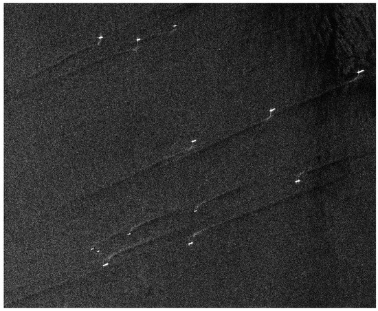
Figure 1. Example of moving ship targets appearing displaced from their wakes in Sentinel-1 image (IW intensity image, VV polarisation).

Among the earliest autofocusing techniques, phase gradient autofocus (PGA) [4] is a very well-known method. It first circularly shifts and windows the data, then uses these processed data to estimate the gradient of the phase errors, and finally integrates the estimations to obtain the phase errors themselves. Mapdrift autofocus is another classical technique for SAR autofocusing [5]. It partitions the whole aperture into several sub-apertures from which the images (maps) are reconstructed, and measures the drift between each pair of maps to obtain the phase errors. These classic methods often serve as the basis for newer methods, such as the variants of the mapdrift and phase gradient autofocus algorithms presented in [6], which employ fractional lower-order moments of the alpha-stable distribution for modelling the phase history data.

Differing from them, various methods based on optimization techniques have been proposed in recent years. Many of these methods belong to one of two categories. The first involves the construction of a sharpness metric to be maximized. For instance, a power function is chosen as the sharpness metric in [7,8], and it is further demonstrated in [8] that when the image is of multiple columns, and under certain statistical assumptions, the perfectly focused image can be closely approximated according to the strong law of large numbers. Image entropy is another popular alternative [9,10,11], though in this case it is minimized (rather than maximized) to enforce sharpness.

The second category of methods adopts an inverse problem approach. Based on a forward observation model associating the corrupted phase history with the underlying SAR image, SAR autofocusing is formulated as an inverse problem, and variational models with a variety of regularizers have been designed to obtain its solution. For instance, Onhon et al. uses the pth power of the approximate $l_p$ norm as the regularization term and an alternating minimization framework to solve the problem [12]. There are also various methods addressing the problem in a compressive sensing context, such as the majorization-minimization-based method [13,14], iteratively re-weighted augmented Lagrangian-based method [15,16] and conjugate gradient-based method with a cost function involving hybrid regularization terms (approximate $l_1$ norm and approximate total variation regularization) [17].

Besides these, there are also SAR autofocusing approaches built by directly strengthening traditional SAR imaging methods. For example, an autofocusing method which maximizes a sharpness metric for each pulse in the imaging process of back-projection is proposed in [18] and further extended to the case of moving ship targets [19]. A polar format algorithm-based autofocusing approach [20] which combines [12] with a classical autofocusing method like PGA has been proposed recently as well.

Moreover, with the development of deep learning, deep neural networks have also recently been considered in SAR autofocusing. A recurrent auto-encoder-based SAR imaging network mimicking the behavior of an iterative shrinkage thresholding algorithm (ISTA) is proposed [21], in which the removal of phase errors is achieved by learning the forward model (observation matrix). Another auto-encoder and decoder-based neural network is built in [22], and the motion compensation is achieved by adding an updating step of the observation matrix in their alternating minimization framework.

In this paper, inspired by [12], we formulate the SAR autofocusing problem as an inverse problem. This enables us to jointly estimate the desired SAR image and the unknown phase errors instead of treating autofocusing as a post-processing step after image reconstruction like traditional autofocusing methods do, thus leading to better performance. In the proposed cost function, we use a non-convex Cauchy regularization on the magnitude of the desired image (thus, we call it “magnitude Cauchy”), exploiting its sparsity-enforcing ability and differentiability. However, this inverse problem poses an interesting challenge in comparison to many other inverse problems in imaging in that it deals with real-valued functions with complex variables. To handle its complex nature, we present two methods for SAR image formation and autofocusing under a framework of alternating minimization. The first method is based on a complex-domain adaptation of the forward-backward splitting algorithm, and is called CFBA. The second method is based on Wirtinger calculus [23,24,25,26] which is designed to deal with differentiable (in the sense of [23]) real-valued functions with complex variables. The second method has been introduced in our previous work [27], referred to as the Wirtinger alternating minimization autofocusing (WAMA) method, but we further give a thorough discussion of its convergence and show that it can be extended to the cases of several other regularizers.

When validating the performance of our methods, we mainly focus on datasets representing the sea surface, i.e., real SAR images containing ships and simulated images of sea surface containing sea wave and ship wakes. The autofocusing of this kind of SAR image can be beneficial for many practical applications, including ship detection [28], the characterization of ship wakes [29], and so on. The source code used to produce the presented results has been made available on GitHub at https://github.com/zy-zhangc/SAR-autofocusing-with-a-non-convex-penalty (accessed on 3 March 2022).

The rest of this paper is organized as follows. In Section 2, a brief introduction is given to the data acquisition model for SAR and the associated problem formulation. In Section 3, the proposed forward-backward splitting-based SAR autofocusing method is described in detail, then its convergence is analyzed. In Section 4, the WAMA method is reviewed, and some more discussion is added, including its extension to the cases of other regularizers and its convergence. In Section 5, experimental results on both simulated scenes and real SAR images are shown to demonstrate the effectiveness of the proposed method. Finally, conclusions are presented in Section 6.

2. SAR Data Acquisition Model

In this paper, a SAR platform operating in spotlight mode is considered, whose transmitted signal at each azimuth position can be expressed as:

$$s(t)=Re\{e^{j({\omega }_{0}t+\alpha t^2)}\},$$

(1)

where ${\omega }_0$ is the carrier frequency, 2$\alpha$ is the chirp rate, and t is fast time.

The obtained data $r_m(t)$ at the mth aperture position and the latent SAR image $F(x,y)$ can be associated by:

$$r_m(t)=\int \int F(x,y)e^{-jU(xcos\theta +ysin\theta )}dxdy.$$

(2)

The region over which the integral is computed is $x^2+y^2\le L^2$, with L being the radius of the circular patch on the ground to be imaged. $\theta$ is the look angle, and U is defined by

$$U=\frac{2}{c}({\omega }_0+2\alpha (t-{\tau }_0)),$$

(3)

with ${\tau }_0$ being the demodulation time. Let M be the number of aperture positions, K be the number of range samples in each range line, and N be the number of pixels of the desired SAR image; then, the discretized version of this model is

$${\mathit{r}}_m={\mathit{C}}_m\mathit{f},m=1,\dots ,M,$$

(4)

where ${\mathit{r}}_m$ and ${\mathit{C}}_m$ are the $K\times 1$ column vector of the phase history and the $K\times N$ observation matrix for the mth aperture position, respectively. $\mathit{f}$ is the $N\times 1$ column vector of the underlying SAR image. Stacking (4) with respect to all the aperture positions, and considering phase errors as well as possible noise, the model becomes

$$\mathit{g}=\mathit{C}(\mathit{\varphi })\mathit{f}+\mathit{n},$$

(5)

with $\mathit{g}$ being the $MK\times 1$ vector of the corrupted phase history, $\mathit{\varphi }$ being the $MK\times 1$ vector of phase errors, and $\mathit{n}$ being the $N\times 1$ vector of Gaussian white noise. $\mathit{C}(\mathit{\varphi })$ is the $MK\times N$ corrupted observation matrix. For more details on this signal model, please see [30,31]. In this paper, only the case of 1D phase errors varying in the azimuth direction is dealt with, which leads to [12]:

$${\mathit{C}}_m(\mathit{\varphi })=e^{j{\mathit{\varphi }}_m}{\mathit{C}}_m,$$

(6)

where ${\mathit{C}}_m(\mathit{\varphi })$ and ${\mathit{\varphi }}_m$ are the corrupted observation sub-matrix for the mth aperture position and the phase error for the mth aperture position, respectively. The case of 2D separable phase errors as well as the case of 2D non-separable phase errors can be formulated similarly; see [12]. For simplicity, we set $MK=N$ in this paper.

3. The Proposed CFBA Method

3.1. The Optimization Model

We formulate SAR autofocusing as an inverse problem and minimize the following cost function:

$$J(\mathit{f},\mathit{\varphi })={\parallel \mathit{g}-\mathit{C}(\mathit{\varphi })\mathit{f}\parallel }_2^2-\lambda \sum _{i=1}^{N}ln\frac{\gamma }{{\gamma }^2+{\left|{\mathit{f}}_i\right|}^2},$$

(7)

where $\lambda$ is the regularization parameter and $\gamma$ is the scale parameter for a Cauchy distribution.

The penalty term in (7) is a Cauchy regularization merely imposed on the magnitude of the latent SAR image. Consequently, we refer to it as “magnitude Cauchy regularization”. Like the $l_p$ norm, it too is a regularization term enforcing statistical sparsity [32], whose effectiveness has already been validated in SAR autofocusing [27], as well as SAR imaging and other inverse problems [33,34].

In (7), the desired SAR image $\mathit{f}$ and the phase errors $\mathit{\varphi }$ are both unknown. By jointly estimating them, SAR image reconstruction and the removal of phase errors are accomplished simultaneously. To do this, we adopt an alternating minimization autofocusing framework similar to [12]. Specifically, $\mathit{f}$ and $\mathit{\varphi }$ are updated alternatively by fixing one of them while optimizing the other. This iterative process will terminate when the relative error between ${\mathit{f}}^{(n)}$ and ${\mathit{f}}^{(n+1)}$ is smaller than ${10}^{-3}$.

3.2. Complex Forward-Backward Splitting-Based Method

Overall, in our alternating minimization framework, we iteratively implement the following two steps:

(1) Image reconstruction step: solve the $\mathit{f}$-sub-problem by

$${\mathit{f}}^{(n+1)}=\arg \underset{\mathit{f}\in {\mathbb{C}}^N}{min}J(\mathit{f},{\mathit{\varphi }}^{(n)});$$

(8)

(2) Phase error estimation step: solve the $\mathit{\varphi }$-sub-problem by

$${\mathit{\varphi }}^{(n+1)}=\arg \underset{\mathit{\varphi }\in {\mathbb{C}}^N}{min}J({\mathit{f}}^{(n+1)},\mathit{\varphi }).$$

(9)

The first step will be detailed in Section 3.2.1, while the second step will be introduced in Section 3.2.2.

3.2.1. Image Reconstruction Step

Under the framework of alternating minimization, each $\mathit{f}$-sub-problem to be solved is

$${\mathit{f}}^{(n+1)}=\arg \underset{\mathit{f}\in {\mathbb{C}}^N}{min}{\parallel \mathit{g}-\mathit{C}({\mathit{\varphi }}^{(n)})\mathit{f}\parallel }_2^2-\lambda \sum _{i=1}^{N}ln\frac{\gamma }{{\gamma }^2+{\left|{\mathit{f}}_i\right|}^2}.$$

(10)

Unlike many other inverse problem formulations in computational imaging, Equation (10) is an optimization problem involving a complex unknown vector, and it thus needs to be handled with appropriate mathematical tools. To this end, we design an iterative solution, which is a complex version of the well-known forward-backward splitting algorithm, and thus we call it complex forward-backward autofocusing (CFBA). It holds the benefit that the computation of the involved complex proximity operators can be converted to the computation of real proximity operators related to the magnitudes of the original complex vector’s components. Therefore, the techniques for real optimization regarding proximal operators can be leveraged. As a result, it is also possible to solve (7) with these techniques when the magnitude Cauchy regularization is replaced by certain non-smooth regularizers. Note that this is not always the case with the WAMA algorithm—the ability to be easily generalised to a number of non-smooth regularizers is a distinct advantage of the CFBA method.

Similar to the forward-backward splitting algorithm for a real case, we recast (10) as

$${\mathit{f}}^{(n+1)}=\arg \underset{\mathit{f}\in {\mathbb{C}}^N}{min}H(\mathit{f})+G(\mathit{f}),$$

(11)

where $H(\mathit{f})= \parallel \mathit{g}-\mathit{C}({\mathit{\varphi }}^{(n)}){\mathit{f}\parallel }_2^2$ and $G(\mathit{f})={\sum }_{i=1}^{N}r({\mathit{f}}_i)=-\lambda {\sum }_{i=1}^{N}ln\frac{\gamma }{{\gamma }^2+{\left|{\mathit{f}}_i\right|}^2}$.

To minimize (11), with a given initial ${\mathit{o}}^{(0)}$, we iteratively implement the following step:

$${\mathit{o}}^{(k+1)}={\mathrm{prox}}_{\mu G}({\mathit{o}}^{(k)}-2\mu {\nabla }_{\mathit{f}}H({\mathit{o}}^{(k)})),$$

(12)

with the proximity operator defined by

$${\mathrm{prox}}_{\mu G}(\mathit{x})=\arg \underset{\mathit{y}\in {\mathbb{C}}^N}{min}\frac{1}{2}{\parallel \mathit{x}-\mathit{y}\parallel }_2^2+\mu G(\mathit{y}),$$

(13)

and the function $\frac{1}{2}{\parallel \mathit{x}-\mathit{y}\parallel }_2^2+\mu G(\mathit{y})$ on its right-hand side is called a Moreau envelope [35]. ${\mathit{f}}^{(n+1)}$ is given by the final output ${\mathit{o}}^{(K)}$ of this inner iterative loop.

In (12), $H(\mathit{f})$ is a real-valued function with a complex vector variable, which is much discussed in Wirtinger calculus. Therefore, instead of using an ordinary gradient operator defined in a real case ∇, here we use the complex gradient operator ${\nabla }_{\mathit{f}}$ defined by Wirtinger calculus. Its definition is first proposed in [23] and further extended in [25]:

$${\nabla }_{\mathit{f}}h={\mathsf{\Omega }}_{\mathit{f}}^{-1}{(\frac{\partial h}{\partial \mathit{f}})}^H.$$

(14)

where ${\mathsf{\Omega }}_{\mathit{f}}^{-1}$ is a metric tensor. Using Brandwood’s setting, i.e., letting it be equal to the identity matrix, we have

$${\nabla }_{\mathit{f}}h={(\frac{\partial h}{\partial \mathit{f}})}^H.$$

(15)

As in (14) and (15), in the rest of this paper, we will use ${\nabla }_{\mathit{f}}$ to denote the complex gradient operator defined by Wirtinger calculus, and ∇ to denote the ordinary gradient operator defined in the real case.

Since the cost function is real-valued, according to [25], we have:

$${(\frac{\partial h}{\partial \mathit{f}})}^H={\overline{(\frac{\partial h}{\partial \mathit{f}})}}^T={(\frac{\partial h}{\partial \overline{\mathit{f}}})}^T={(\frac{\partial h}{\partial \overline{{\mathit{f}}_1}},\dots ,\frac{\partial h}{\partial \overline{{\mathit{f}}_N}})}^T.$$

(16)

The last term in the right side of (16) can be computed using the chain rule and the definition of the conjugate $\mathbb{R}$-derivative, i.e., $\frac{\partial h}{\partial \overline{{\mathit{f}}_i}}=\frac{1}{2}(\frac{\partial h}{\partial {\mathit{x}}_i}+i\frac{\partial h}{\partial {\mathit{y}}_i})$, with ${\mathit{x}}_i$ and ${\mathit{y}}_i$ being the real and imaginary part of ${\mathit{f}}_i$, respectively [25].

It should also be noted that in (12), the step size is written as $2\mu$ rather than the commonly used $\mu$ in the real-case forward-backward splitting algorithm. This choice is implied by the relationship between the complex gradient ${\nabla }_{\mathit{f}}$ and real gradient ∇; see e.g., [23]. Furthermore, $\mu$ should satisfy $\mu \le \frac{1}{L}$, as will be further discussed in Section 3.2.

As a result of Wirtinger calculus, it can be shown that

$${\nabla }_{\mathit{f}}H(\mathit{f})=\mathit{C}{({\mathit{\varphi }}^{(n)})}^H(\mathit{C}({\mathit{\varphi }}^{(n)})\mathit{f}-\mathit{g}).$$

(17)

As for the computation of (13), we first expand it as

$${\mathrm{prox}}_{\mu G}(\mathit{x})=\arg \underset{\mathit{y}\in {\mathbb{C}}^N}{min}\frac{1}{2}\sum _{i=1}^N{|{\mathit{x}}_i-{\mathit{y}}_i|}^2-\mu \lambda \sum _{i=1}^{N}ln\frac{\gamma }{{\gamma }^2+{\left|{\mathit{y}}_i\right|}^2}.$$

(18)

Then we solve (18) by independently solving

$${\mathrm{prox}}_{\mu \lambda r}({\mathit{x}}_i)=\arg \underset{{\mathit{y}}_i\in \mathbb{C}}{min}\frac{1}{2}{|{\mathit{x}}_i-{\mathit{y}}_i|}^2-\mu \lambda ln\frac{\gamma }{{\gamma }^2+{\left|{\mathit{y}}_i\right|}^2}$$

(19)

for each $i(i=1,\dots ,N)$.

For (19), observe that the logarithm term in the Moreau envelope merely depends on $|{\mathit{y}}_i|$; thus the solution ${\mathit{y}}_i^{*}$ must lie on the line passing through the origin and the input ${\mathit{x}}_i$, as long as ${\mathit{x}}_i$ is not 0. When searching among all the ${\mathit{y}}_i$ for ${\mathit{y}}_i^{*}$, if $|{\mathit{y}}_i|$ is fixed, then only the first term of (19) needs to be minimized, since the second term therein is a constant in this case. To minimize the former, we just need to find the point on a circle with radius $|{\mathit{y}}_i|$ in the complex plane which is closest to the fixed point ${\mathit{x}}_i$. Obviously, this point would be the one which also lies on the line passing through the origin and ${\mathit{x}}_i$, if ${\mathit{x}}_i$ is not 0. Therefore, the desired point will have the same argument as ${\mathit{x}}_i$. Since the choice of $|{\mathit{y}}_i|$ is arbitrary, the argument of ${\mathit{y}}_i^{*}$ must be the same as that of ${\mathit{x}}_i$.

However, if ${\mathit{x}}_i=0$, every ${\mathit{y}}_i$ on a certain circle of the complex plane will be the solution of (19). In this case, we set the argument of ${\mathit{y}}_i$ as 0, as in [35].

Therefore, the solution of (19) can now be split into two steps. The first is to solve the corresponding real optimization problem which gives $|{\mathit{y}}_i^{*}|$:

$$|{\mathit{y}}_i^{*}|=\arg \underset{y\in \mathbb{R}}{min}\frac{1}{2}(|{\mathit{x}}_i{|-y)}^2-\mu \lambda ln\frac{\gamma }{{\gamma }^2+y^2}.$$

(20)

The second step is to let

$${\mathit{y}}_i^{*}=\left\{\begin{array}{cc}|{\mathit{y}}_i^{*}|e^{j{\varphi }_{{\mathit{x}}_i}}\hfill & {\mathit{x}}_i\ne 0\hfill \\ |{\mathit{y}}_i^{*}|\hfill & {\mathit{x}}_i=0\hfill \end{array}\right.$$

(21)

where $e^{j{\varphi }_{{\mathit{x}}_i}}={\mathit{x}}_i/\left|{\mathit{x}}_i\right|$. Similar techniques can also be seen in phase retrieval [35] and SAR imaging [36].

Note that (20) is a non-convex optimization problem. If we compute the gradient of the Moreau envelope in the right-hand side and set it to 0, we will get a cubic equation. It may have three real roots, which stands for three stationary points. Here, however, we can add some constraints to simplify the problem. By restricting $\gamma >\frac{\sqrt{\mu \lambda }}{2}$, this Moreau envelope becomes strictly convex and thus implies the existence of only one, real stationary point [34]. In this case, the corresponding cubic equation must have a single real root and a pair of complex roots, and since our desired solution is a magnitude, then the solution we seek must be the real root. This real root is given by [33]:

$$|{\mathit{y}}_i^{*}|=\frac{|{\mathit{x}}_i|}{3}+s+t,$$

(22)

where

$$s=\sqrt[3]{\frac{q}{2}+\sqrt{\frac{p^3}{27}+\frac{q^2}{4}}},$$

(23)

$$t=\sqrt[3]{\frac{q}{2}-\sqrt{\frac{p^3}{27}+\frac{q^2}{4}}},$$

(24)

$$p={\gamma }^2+2\mu \lambda -\frac{|{\mathit{x}}_i{|}^2}{3},$$

(25)

$$q={\gamma }^2\left|{\mathit{x}}_i\right|+\frac{2|{\mathit{x}}_i{|}^3}{27}-\frac{{\gamma }^2+2\mu \lambda }{3}\left|{\mathit{x}}_i\right|.$$

(26)

3.2.2. Optimization of the Phase Errors

After obtaining each ${\mathit{f}}^{(n+1)}$, we use it to compute ${\mathit{\varphi }}^{(n+1)}$. For 1D phase errors varying along the azimuth direction, the vector of phase errors can be updated by solving the following sequence of sub-problems concerning its components:

$${\mathit{\varphi }}_m^{(n+1)}=\arg \underset{{\mathit{\varphi }}_m}{min}{\parallel {\mathit{g}}_m-e^{j{\mathit{\varphi }}_m}{\mathit{C}}_m{\mathit{f}}^{(n+1)}\parallel }_2^2,m=1,\dots ,N,$$

(27)

with ${\mathit{g}}_m$ and ${\mathit{C}}_m$ being the parts of $\mathit{g}$ and $\mathit{C}$ corresponding to the mth aperture position. According to [12], the solution is

$${\mathit{\varphi }}_m^{(n+1)}=arctan(\frac{\mathrm{Re}\{{[{\mathit{f}}^{(n+1)}]}^H{\mathit{C}}_m{\mathit{g}}_m\}}{\mathrm{Im}\{{[{\mathit{f}}^{(n+1)}]}^H{\mathit{C}}_m{\mathit{g}}_m\}}).$$

(28)

The corrupted observation matrix can then be estimated by:

$${\mathit{C}}_m({\mathit{\varphi }}_m^{(n+1)})=e^{j{\mathit{\varphi }}_m^{(n+1)}}{\mathit{C}}_m.$$

(29)

The cases of 2D phase errors varying in both range direction and cross-range direction can also be solved by similar methods; see [12] for more details. The whole process of the proposed CFBA method is summarized in Algorithm 1.

We point out here that CFBA differs from  [33] mainly in two aspects. First, the authors of the other study do not deal with the same problem. The method in [33] is applied to SAR imaging, while CFBA addresses a different and more challenging problem, i.e., SAR autofocusing, which removes phase errors and reconstructs SAR image simultaneously. Second, only part of the solving process in CFBA is inspired by [33]. When facing each f-sub-problem of CFBA, techniques similar to [35,36] are used to tackle the complex nature of the problem, which makes it possible to handle the magnitudes and the arguments of the components of the complex solution separately. On the basis of this, Formulas (22)–(26) in [33] are utilized to facilitate the computation of the magnitudes.

Algorithm 1: CFBA

Initialize $n=0$, ${\mathit{f}}^{(0)}={\mathit{C}}^H\mathit{g}$, ${\mathit{\varphi }}^{(0)}=0$, $\mathit{C}({\mathit{\varphi }}^0)=\mathit{C}$, and set the values of $\gamma$, $\lambda$, and $\mu$ according to $\mu \in (0,\frac{1}{L})$ and $\gamma \ge \frac{\sqrt{\mu \lambda }}{2}$ while$n<300$ or $\parallel {\mathit{f}}^{(n+1)}-{\mathit{f}}^{(n)}\parallel /\parallel {\mathit{f}}^{(n)}\parallel >0.001$ do     1. Compute ${\mathit{f}}^{(n+1)}$ by complex forward-backward splitting method, i.e.,     while $k<500$ or $\parallel {\mathit{o}}^{(k+1)}-{\mathit{o}}^{(k)}\parallel /\parallel {\mathit{o}}^{(k)}\parallel >0.001$ do         Find ${\mathit{o}}^{(k+1)}={\mathrm{prox}}_{\lambda \mu R}({\mathit{o}}^{(k)}-\mu \mathit{C}{({\mathit{\varphi }}^{(n)})}^H(\mathit{C}({\mathit{\varphi }}^{(n)}){\mathit{o}}^{(k)}-\mathit{g}))$ by (20)–(26)         $k=k+1$     end while     2. Compute ${\varphi }_m^{(n+1)}$ by (28)     3. Compute $\mathit{C}({\mathit{\varphi }}_m^{(n+1)})$ by (29)     4. $n=n+1$ end while

3.3. Convergence Analysis

For the proposed CFBA method, the issue of convergence is twofold. That is to say, the discussion needs to cover the convergence of the inner complex forward-backward splitting algorithm as well as the convergence of the outer alternating minimization algorithm.

3.3.1. Convergence of the Inner Complex Forward-Backward Splitting Algorithm

In the nth image reconstruction step, we find

$${\mathit{f}}^{(n+1)}=\arg \underset{\mathit{f}\in {\mathbb{C}}^N}{min}{\parallel \mathit{g}-\mathit{C}({\mathit{\varphi }}^{(n)})\mathit{f}\parallel }_2^2-\lambda \sum _{i=1}^{N}ln\frac{\gamma }{{\gamma }^2+{\left|{\mathit{f}}_i\right|}^2},$$

(30)

and in each step of the complex FB splitting algorithm which solves (30) iteratively, we compute

$${\mathit{o}}^{(k+1)}=\arg \underset{\mathit{o}\in {\mathbb{C}}^N}{min}\frac{1}{2}{\parallel \mathit{o}-{\mathit{z}}^{(k)}\parallel }_2^2-\mu \lambda \sum _{i=1}^{N}ln\frac{\gamma }{{\gamma }^2+{\left|{\mathit{o}}_i\right|}^2},$$

(31)

where

$${\mathit{z}}^{(k)}={\mathit{o}}^{(k)}-2\mu \mathit{C}{({\mathit{\varphi }}^{(n)})}^H(\mathit{C}({\mathit{\varphi }}^{(n)}){\mathit{o}}^{(k)}-\mathit{g}).$$

(32)

Since ${\mathit{\varphi }}^{(n)}$ is fixed for the nth f-sub-problem, for simplicity of notation, we will denote $\mathit{C}({\mathit{\varphi }}^{(n)})$ by ${\mathit{C}}^{(n)}$ in this subsection. Using the notations of (11), we denote the cost function in (30) as $J_n(\mathit{f})=H(\mathit{f})+G(\mathit{f})$, with $H(\mathit{f})=\parallel \mathit{g}-{\mathit{C}}^{(n)}{\mathit{f}\parallel }_2^2$ and $G(\mathit{f})=-\lambda {\sum }_{i=1}^{N}ln\frac{\gamma }{{\gamma }^2+{\left|{\mathit{f}}_i\right|}^2}$.

Now, note that for an arbitrary N-dimensional $\mathit{f}={({\mathit{f}}_1,\dots ,{\mathit{f}}_N)}^T={({\mathit{x}}_1+i{\mathit{y}}_1,\dots ,{\mathit{x}}_N+i{\mathit{y}}_N)}^T\in {\mathbb{C}}^N$, we can obtain a $2N$-dimensional real vector $\tilde{\mathit{f}}={({\mathit{x}}_1,\dots ,{\mathit{x}}_N,{\mathit{y}}_1,\dots ,{\mathit{y}}_N)}^T\in {\mathbb{R}}^{2N}$. Conversely, for an arbitrary $2N$-dimensional $\tilde{\mathit{f}}={({\tilde{\mathit{f}}}_1,\dots ,{\tilde{\mathit{f}}}_N,{\tilde{\mathit{f}}}_{N+1},\dots ,{\tilde{\mathit{f}}}_{2N})}^T\in {\mathbb{R}}^{2N}$, we can obtain a N-dimensional complex vector $\mathit{f}={({\mathit{f}}_1,\dots ,{\mathit{f}}_N)}^T={({\tilde{\mathit{f}}}_1+i{\tilde{\mathit{f}}}_{N+1},\dots ,{\tilde{\mathit{f}}}_N+i{\tilde{\mathit{f}}}_{2N})}^T\in {\mathbb{C}}^N$. For simplicity, we denote ${\tilde{\mathit{f}}}_R={({\tilde{\mathit{f}}}_1,\dots ,{\tilde{\mathit{f}}}_N)}^T$ and ${\tilde{\mathit{f}}}_I={({\tilde{\mathit{f}}}_{N+1},\dots ,{\tilde{\mathit{f}}}_{2N})}^T$ for $\tilde{\mathit{f}}$. With these notations, we give the following lemma.

Lemma 1.

$J_n(\mathit{f})$ can be rewritten as ${\tilde{J}}_n(\tilde{\mathit{f}})$, which is a real analytic function.

The proof of this lemma is put in Appendix A.

Now, since $\widetilde{J_n}(\tilde{\mathit{f}})$ is real analytic, it satisfies the Kurdyka–Lojasiewicz (KL) property [37], which means that for every $\tilde{\mathit{f}}{}^{\prime }\in {\mathbb{R}}^{2N}$ and every bounded neighborhood U of $\tilde{\mathit{f}}{}^{\prime }$, there exists $\kappa \in (0,+\infty )$, $\eta \in (0,+\infty )$ and $\theta \in [0,1)$ such that

$$\parallel \nabla \widetilde{J_n}(\tilde{\mathit{f}})\parallel \ge \kappa |\widetilde{J_n}(\tilde{\mathit{f}})-\widetilde{J_n}(\tilde{\mathit{f}}{}^{\prime }){|}^{\theta }$$

(33)

for every $\tilde{\mathit{f}}\in U\cap \{\tilde{\mathit{f}}\left|\right|\widetilde{J_n}(\tilde{\mathit{f}})-\widetilde{J_n}(\tilde{\mathit{f}}{}^{\prime })|\le \eta \}$.

The proof of Lemma 1 also implies the proof of the convergence of the CFBA algorithm from a perspective of real vector variables, because $J_n(\mathit{f})$ (a function of the complex $\mathit{f}$) can now be viewed as $\widetilde{J_n}(\tilde{\mathit{f}})$ (a function of real vector variable $\tilde{\mathit{f}}$). If the real forward-backward splitting algorithm minimizing $\widetilde{J_n}(\tilde{\mathit{f}})$ can be connected with the proposed complex forward-backward splitting algorithm minimizing $J_n(\mathit{f})$, then the convergence analysis of the latter will benefit from the convergence analysis of the former.

Theorem 1.

Note that $k\to +\infty$, ${\mathit{o}}^{(k)}$ generated by (31) will converge to some critical point of $J_n(\mathit{f})$. Moreover, denote by ${\mathit{f}}^{*}$ the global minimizer of $J_n(\mathit{f})$; then for each $r>0$, there exist $u\in (0,r),$$\delta >0$ such that when the inequalities $min{J}_n(\mathit{f})<J_n({\mathit{o}}^{(0)})<\delta +min{J}_n(\mathit{f})$ and $\parallel {\mathit{o}}^{(0)}-{\mathit{f}}^{*}\parallel < u$ hold, the sequence ${\mathit{o}}^{(k)}$ generated for each $J_n(\mathit{f})$ will converge to some ${\mathit{o}}^{*}$ with ${\mathit{o}}^{(k)}\in B({\mathit{f}}^{*},r)$ for an arbitrary k and $J_n({\mathit{u}}^{*})=min{J}_n(\mathit{f})$.

Proof. 

Let us first formulate the real forward-backward splitting algorithm minimizing ${\tilde{J}}_n(\tilde{\mathit{f}})$ with respect to $\tilde{\mathit{f}}$. First denote ${\mathit{u}}^{(0)}=\widetilde{{\mathit{o}}^{(0)}}$. Then in each step, this algorithm finds

$$\begin{array}{c}\hfill {\mathit{u}}^{(k+1)}={\mathrm{prox}}_{\mu \tilde{G}}({\mathit{w}}^{(k)})=\arg \underset{\mathit{u}\in {\mathbb{R}}^{2N}}{min}\frac{1}{2}{\parallel \mathit{u}-{\mathit{w}}^{(k)}\parallel }_2^2-\mu \lambda \sum _{i=1}^{N}ln\frac{\gamma }{{\gamma }^2+{\parallel {\mathit{s}}_{(i)}\mathit{u}\parallel }^2},\end{array}$$

(34)

where

$${\mathit{w}}^{(k)}={\mathit{u}}^{(k)}-2\mu {\widetilde{{\mathit{C}}^{(n)}}}^T(\widetilde{{\mathit{C}}^{(n)}}{\mathit{u}}^{(k)}-\tilde{\mathit{g}}).$$

(35)

Observe that

$${({\mathit{C}}^{(n)})}^H\mathit{f}={(\overline{c_{11}}{\mathit{f}}_1+\cdots +\overline{c_{N1}}{\mathit{f}}_N,\dots ,\overline{c_{1N}}{\mathit{f}}_1+\cdots +\overline{c_{NN}}{\mathit{f}}_N)}^T,$$

(36)

and

$$\tilde{{({\mathit{C}}^{(n)})}^H\mathit{f}}=\left(\begin{array}{c}{(c_{11})}_R{\mathit{x}}_1+{(c_{11})}_I{\mathit{y}}_1+\cdots +{(c_{N1})}_R{\mathit{x}}_N+{(c_{N1})}_I{\mathit{y}}_N\\ ⋮\\ {(c_{1N})}_R{\mathit{x}}_1+{(c_{1N})}_I{\mathit{y}}_1+\cdots +{(c_{NN})}_R{\mathit{x}}_N+{(c_{NN})}_I{\mathit{y}}_N\\ {(-c_{11})}_I{\mathit{x}}_1+{(c_{11})}_R{\mathit{y}}_1+\cdots +{(-c_{N1})}_I{\mathit{x}}_N+{(c_{N1})}_R{\mathit{y}}_N\\ ⋮\\ {(-c_{1N})}_I{\mathit{x}}_1+{(c_{1N})}_R{\mathit{y}}_1+\cdots +{(-c_{NN})}_I{\mathit{x}}_N+{(c_{NN})}_R{\mathit{y}}_N\end{array}\right).$$

(37)

This can be exactly decomposed as

$$\tilde{{({\mathit{C}}^{(n)})}^H\mathit{f}}={\widetilde{{\mathit{C}}^{(n)}}}^T\tilde{\mathit{f}},$$

(38)

where $\widetilde{{\mathit{C}}^{(n)}}$ is as in (A5).

Therefore, we have

$${\mathit{w}}^{(0)}=\widetilde{{\mathit{o}}^{(0)}}-2\mu {\widetilde{{\mathit{C}}^{(n)}}}^T(\widetilde{{\mathit{C}}^{(n)}}\widetilde{{\mathit{o}}^{(0)}}-\tilde{\mathit{g}})=\widetilde{{\mathit{o}}^{(0)}}-2\mu \widetilde{\nabla h({\mathit{o}}^{(0)})}=\widetilde{{\mathit{z}}^{(0)}},$$

(39)

with ${\mathit{z}}^{(0)}$ defined by (32) for CFBA.

If now we rewrite the $\mathit{u}$ in (34) by $\mathit{u}=\tilde{\mathit{o}}$, then the Moreau envelope therein becomes a function of $\tilde{\mathit{o}}$. Additionally, if this function is rewritten as a function of $\mathit{o}$, the result will exactly take the form of the Moreau envelope in (31). Moreover, we have $\nabla \widetilde{J_n}(\tilde{\mathit{f}})={({(\frac{\partial \widetilde{J_n}}{\partial {\tilde{\mathit{f}}}_R})}^T,{(\frac{\partial \widetilde{J_n}}{\partial {\tilde{\mathit{f}}}_I})}^T)}^T$ by the definition of the real gradient and ${\nabla }_{\mathit{f}}{J}_n(\mathit{f})=\frac{1}{2}(\frac{\partial \widetilde{J_n}}{\partial {\tilde{\mathit{f}}}_R}+i\frac{\partial \widetilde{J_n}}{\partial {\tilde{\mathit{f}}}_I})$ by the definition in Wirtinger calculus. Therefore, if $\mathit{f}$ is a stationary point of $J_n(\mathit{f})$, then the corresponding $\tilde{\mathit{f}}$ is a stationary point of $\widetilde{J_n}(\tilde{\mathit{f}})$. Since we have forced convexity of the Moreau envelopes in (34) and (31) by restricting the range of parameters, they will each have only one stationary point. Due to these three conclusions, ${\mathit{u}}^{(1)}=\widetilde{{\mathit{o}}^{(1)}}$ holds.

By induction, following similar deduction, a sequence ${\mathit{o}}^{(k)}$ complying with (31) in the CFBA algorithm and meanwhile satisfying ${\mathit{u}}^{(k)}=\widetilde{{\mathit{o}}^{(k)}}$ for all k can be obtained. Therefore, the convergence of the CFBA algorithm can be analyzed equivalently by discussing this real FB splitting algorithm.

The analysis above also implies that the nth f-sub-problem can be solved by finding the corresponding real solution for $\widetilde{J_n}(\tilde{\mathit{f}})$ and transforming it back to the desired complex solution. However, the proposed CFBA algorithm is more compact in form, since it deals with N dimensional vectors instead of $2N$ dimensional vectors, and it does not require the construction of $\tilde{C}$ based on C.

Now, ${\tilde{J}}_n(\tilde{\mathit{f}})=\tilde{G}(\tilde{\mathit{f}})+\tilde{H}(\tilde{\mathit{f}})$ is proper and lower semicontinuous, bounded from below if hyper-parameters are chosen appropriately (by selecting $\lambda >0$ and $\gamma <1$, we have ${\tilde{J}}_n(\tilde{\mathit{f}})>\lambda Nln\gamma$), and it satisfies the KL property. $\tilde{H}(\tilde{\mathit{f}})$ is finite-valued, differentiable, and has a Lipschitz continuous gradient. Moreover, $\tilde{G}(\tilde{\mathit{f}})$ is continuous on its domain. That is to say, all the conditions in Theorem 5.1 of [38] are satisfied. Therefore, according to that theorem, with the conditions aforementioned and the setting $\mu \le \frac{1}{L}$ (which guarantees the monotonic decreasing nature of ${\tilde{J}}_n({\mathit{u}}^{(k)})$), we come to the conclusion that the iterates ${\mathit{u}}^{(k)}$ will converge to some critical point of ${\tilde{J}}_n(\tilde{\mathit{f}})$. Therefore, equivalently, the iterates ${\mathit{o}}^{(k)}$ produced by the proposed CFBA method will converge to some critical point of $J_n(\mathit{f})$.

Moreover, let us denote by ${\tilde{\mathit{f}}}^{*}$ the global minimizer of ${\tilde{J}}_n(\tilde{\mathit{f}})$. According to Theorem 2.12 in [38], for each $r>0$, there exist $u\in (0,r),\delta >0$ such that when the inequalities $\parallel {\mathit{u}}^{(0)}-{\tilde{\mathit{f}}}^{*}\parallel < u$ and $min{\tilde{J}}_n(\tilde{\mathit{f}})<{\tilde{J}}_n({\mathit{u}}^{(0)})<\delta +min{\tilde{J}}_n(\tilde{\mathit{f}})$ hold, the sequence ${\mathit{u}}^{(k)}$ generated for each ${\tilde{J}}_n(\tilde{\mathit{f}})$ will converge to some ${\mathit{u}}^{*}$ with ${\mathit{u}}^{(k)}\in B({\tilde{\mathit{f}}}^{*},r)$ for arbitrary k and ${\tilde{J}}_n({\mathit{u}}^{*})=min{\tilde{J}}_n(\tilde{\mathit{f}})$. That is to say, under some assumptions about the initial value ${\mathit{u}}^{(0)}$, convergence of the sequence ${\mathit{u}}^{(k)}$ to a global minimizer of ${\tilde{J}}_n(\tilde{\mathit{f}})$ can be obtained. Equivalently, for each $r>0$, there exist $u\in (0,r),\delta >0$ such that when the inequalities $\parallel {\mathit{o}}^{(0)}-{\mathit{f}}^{*}\parallel < u$ and $min{J}_n(\mathit{f})<J_n({\mathit{o}}^{(0)})<\delta +min{J}_n(\mathit{f})$ hold, the sequence ${\mathit{o}}^{(k)}$ generated for each $J_n(\mathit{f})$ will converge to some ${\mathit{o}}^{*}$ with ${\mathit{o}}^{(k)}\in B({\mathit{f}}^{*},r)$ for arbitrary k and $J_n({\mathit{u}}^{*})=min{J}_n(\mathit{f})$, i.e., the iterates ${\mathit{o}}^{(k)}$ produced by the proposed CFBA method will converge to a global minimizer of $J_n(\mathit{f})$. □

In fact, the above proof, which is elaborated from a real perspective, can also be done alternatively by working on the complex iterates ${\mathit{o}}^{(k)}$ themselves. However, this process is more complicated (see Appendix A).

3.3.2. Convergence of the Outer Alternating Minimization Method

Based on Theorem 1, the following result can be obtained:

Theorem 2.

For each $\mathit{f}$-sub-problem, if the assumptions related to the initial value ${\mathit{o}}^{(0)}$ stated in Theorem 1 are satisfied, with ${\mathit{f}}^{(n)}$ and ${\mathit{\varphi }}^{(n)}$ computed by CFBA, $J({\mathit{f}}^{(n)},{\mathit{\varphi }}^{(n)})$ will converge to a certain value (not necessarily equal to $infJ(\mathit{f},\mathit{\varphi })$).

Proof. 

For each $\mathit{f}$-sub-problem, if the assumptions related to the initial value ${\mathit{o}}^{(0)}$ stated in the last section are satisfied, the sequence ${\mathit{o}}^{(k)}$ will converge to a global minimizer of $J_n(\mathit{f})$. In this case, $J({\mathit{f}}^{(n+1)},{\mathit{\varphi }}^{(n)})\le J({\mathit{f}}^{(n)},{\mathit{\varphi }}^{(n)})$. Additionally, since each $\varphi$-sub-problem has a closed form solution, we have $J({\mathit{f}}^{(n+1)},{\mathit{\varphi }}^{(n+1)})\le J({\mathit{f}}^{(n+1)},{\mathit{\varphi }}^{(n)})$. As a result, $J({\mathit{f}}^{(n+1)},{\mathit{\varphi }}^{(n+1)})\le J({\mathit{f}}^{(n)},{\mathit{\varphi }}^{(n)})$ holds for every n, i.e., $J({\mathit{f}}^{(n)},{\mathit{\varphi }}^{(n)})$ is a monotonically decreasing sequence. Since it is also bounded below, it will converge to a certain value, though not necessarily equal to $infJ(\mathit{f},\mathit{\varphi })$. □

If stronger assumptions are satisfied, better results of convergence can be obtained. For instance, if the five-point property [39,40] holds, i.e., if

$$J(\mathit{f},\mathit{\varphi })+J(\mathit{f},{\mathit{\varphi }}^{(n)})\ge J(\mathit{f},{\mathit{\varphi }}^{(n+1)})+J({\mathit{f}}^{(n+1)},{\mathit{\varphi }}^{(n)})$$

(40)

holds for every $\mathit{f},\mathit{\varphi }$, and n, then

$$\underset{n\to +\infty }{lim}J({\mathit{f}}^{(n)},{\mathit{\varphi }}^{(n)})=infJ(\mathit{f},\mathit{\varphi }).$$

(41)

4. Wirtinger Alternating Minimization Autofocusing

4.1. The Original Method

In this section, we review the Wirtinger alternating minimization autofocusing (WAMA) method originaly proposed in [27]. After that, we briefly expand on how to extend this method to several other cost functions with the same fidelity term but with different regularizers. Finally, we will discuss the convergence of this method, a topic not covered in previous publications.

The WAMA method also adopts the framework of alternating minimization, including two types of sub-problems to be solved. For each $\mathit{f}$-sub-problem formulated in (10), Wirtinger calculus is used to solve it. On the one hand, Wirtinger calculus is a powerful theory covering the analysis of real-valued functions of complex variables, and within which many real optimization problems can have their complex counterparts defined. On the other hand, it is also a rather elegant approach, due to its ability to address the problem in a concise way. Namely, there is no need to expand the complex variables as real vectors in the computational process.

Specifically, to solve (10), we compute the complex gradient of the cost function therein directly using Wirtinger calculus. Using the notation in Section 3.2.1, we have

$${({\nabla }_{\mathit{f}}G(\mathit{f}))}_i=\frac{\lambda {\mathit{f}}_i}{{\gamma }^2+{\left|{\mathit{f}}_i\right|}^2},i=1,\dots ,N.$$

(42)

Since ${\nabla }_{\mathit{f}}H(\mathit{f})$ is already given in (17), the complex gradient of (10) can be written as:

$${\nabla }_{\mathit{f}}J(\mathit{f},\mathit{\varphi })=\mathit{C}{({\mathit{\varphi }}^{(n)})}^H(\mathit{C}({\mathit{\varphi }}^{(n)})\mathit{f}-\mathit{g})+\lambda \mathit{W}(\mathit{f})\mathit{f},$$

(43)

where

$$\mathit{W}(\mathit{f})=\mathrm{diag}(\mathit{s}),$$

(44)

$${\mathit{s}}_i=\frac{1}{{\gamma }^2+{\left|{\mathit{f}}_i\right|}^2},i=1,\dots ,N.$$

(45)

Now we set (43) to zero, according to the necessary and sufficient condition for a stationary point of a real-valued complex function [23,25], which leads to

$$[\mathit{C}{({\mathit{\varphi }}^{(n)})}^H\mathit{C}({\mathit{\varphi }}^{(n)})+\lambda \mathit{W}(\mathit{f})]\mathit{f}=\mathit{C}{({\mathit{\varphi }}^{(n)})}^H\mathit{g}.$$

(46)

It is worth pointing out that even though the exact solution of (46) can be obtained, that solution is not necessarily the global minimum of (10) due to the non-convexity of the Cauchy penalty.

Now we rewrite (46) as $\mathit{A}\mathit{f}=\mathit{b}$, where $\mathit{A}=\lambda \mathit{W}(\mathit{f})+\mathit{C}{({\mathit{\varphi }}^{(n)})}^H\mathit{C}({\mathit{\varphi }}^{(n)})$ and $\mathit{b}=\mathit{C}{({\mathit{\varphi }}^{(n)})}^H\mathit{g}$. Since $\mathit{W}(\mathit{f})$ depends on $\mathit{f}$, so does $\mathit{A}$. This makes (46) nonlinear with respect to $\mathit{f}$, and it is difficult to find its closed-form solution. However, if we sacrifice some accuracy and approximate the $\mathit{f}$ in $\mathit{W}(\mathit{f})$ with the $\mathit{f}$ computed during the last iteration of the alternating minimization framework, $\mathit{A}$ is converted into a constant matrix, and thus $\mathit{A}\mathit{f}=\mathit{b}$ becomes a linear system of equations which can be solved efficiently.

That is to say, when computing an unknown ${\mathit{f}}^{(n+1)}$, the actually solved equation is

$$[\mathit{C}{({\mathit{\varphi }}^{(n)})}^H\mathit{C}({\mathit{\varphi }}^{(n)})+\lambda \mathit{W}({\mathit{f}}^{(n)})]{\mathit{f}}^{(n+1)}=\mathit{C}{({\mathit{\varphi }}^{(n)})}^H\mathit{g}.$$

(47)

This equation can be viewed as a fixed-point algorithm with a single iterative step, and its solution can be efficiently obtained by using the conjugate gradient (CG) algorithm [41]. The experimental results in Section 5 imply that the obtained solution is sufficiently good.

As for the $\mathit{\varphi }$-sub-problems, the solutions are the same as that of CFBA introduced in Section 3.1, so they are not presented here. Now, the whole process of the WAMA method can be summarized as Algorithm 2 as follows:

Algorithm 2: WAMA

Initialize $n=0$, ${\mathit{f}}^{(0)}={\mathit{C}}^H\mathit{g}$, ${\mathit{\varphi }}^{(0)}=0$, $\mathit{C}({\mathit{\varphi }}^0)=\mathit{C}$, and set the values of $\gamma$ and $\lambda$ while $n<300$ or $\parallel {\mathit{f}}^{(n+1)}-{\mathit{f}}^{(n)}\parallel /\parallel {\mathit{f}}^{(n)}\parallel >0.001$ do     1. Compute ${\mathit{f}}^{(n+1)}$ by finding the solution of (47) via CG     2. Compute ${\mathit{\varphi }}_m^{(n+1)}$ by (28)     3. Compute $\mathit{C}({\mathit{\varphi }}_m^{(n+1)})$ by (29)     4. $n=n+1$ end while

4.2. Extension to Several Other Regularizers

As an extension, the same computational processes can also be followed to handle the cases where the magnitude Cauchy regularization in (7) is replaced by some other $\mathbb{R}$-differentiable regularizers [25]. For those cases, Equation (47) will also be obtained, despite the fact that the involved $\mathit{s}$ is different. We give several examples as follows:

(1)

The pth power of an approximate $l_p$ norm

In this case,

$$G(\mathit{f})=\lambda \sum _{i=1}^N(|{\mathit{f}}_i{{|}^2+\beta )}^{\frac{p}{2}},$$

(48)

and now

$${\mathit{s}}_i=\frac{p}{2(|{\mathit{f}}_i{{|}^2+\beta )}^{1-\frac{p}{2}}},i=1,\dots ,N.$$

(49)

This yields the same algorithm as in this case of [12], but no reference to the literature of Wirtinger calculus is made therein. Therefore, this deduction can be viewed as an alternative perspective to interpret SDA;

(2)

Approximate total variation

For approximate total variation, the situation is more complicated. However, the result can still be incorporated in the form of (47). Let $\mathit{F}$ be the 2D $a\times a$ matrix form of the N-dimensional vector $\mathit{f}(N=a\times a)$; then

$$G(\mathit{f})=\lambda \sum _{i=1}^a\sum _{j=1}^a\sqrt{|{({\nabla }_i\mathit{F})}_{i,j}{|}^2+{\left|{({\nabla }_j\mathit{F})}_{i,j}\right|}^2+\beta },$$

(50)

with

$${({\nabla }_i\mathit{F})}_{i,j}=\left\{\begin{array}{cc}{\mathit{F}}_{i,j}-{\mathit{F}}_{i-1,j}\hfill & i>1\hfill \\ 0\hfill & i=1\hfill \end{array}\right.$$

(51)

$${({\nabla }_j\mathit{F})}_{i,j}=\left\{\begin{array}{cc}{\mathit{F}}_{i,j}-{\mathit{F}}_{i,j-1}\hfill & j>1\hfill \\ 0\hfill & j=1\hfill \end{array}\right.$$

(52)

Now

$$\mathit{W}(\mathit{f})={\mathit{W}}^{{}^{\prime }}{\mathit{D}}^{{}^{\prime }}+{\mathit{W}}^{{}^{\prime }}{\mathit{D}}^{{}^{″}}+{\mathit{W}}^{{}^{″}}{\mathit{D}}^{{}^{‴}}+{\mathit{W}}^{{}^{‴}}{\mathit{D}}^{{}^{⁗}},$$

(53)

$${\mathit{W}}^{{}^{\prime }}=\mathrm{diag}(\mathrm{vec}({\mathit{S}}^{{}^{\prime }})),{\mathit{W}}^{{}^{″}}=\mathrm{diag}(\mathrm{vec}({\mathit{S}}^{{}^{″}})),{\mathit{W}}^{{}^{‴}}=\mathrm{diag}(\mathrm{vec}({\mathit{S}}^{{}^{‴}})),$$

(54)

where vec is the operation which turns a matrix into a column vector by stacking its columns in order. Additionally,

$${({\mathit{S}}^{{}^{\prime }})}_{i,j}=\frac{1}{2\sqrt{|{({\nabla }_i\mathit{F})}_{i,j}{|}^2+{\left|{({\nabla }_j\mathit{F})}_{i,j}\right|}^2+\beta }},$$

(55)

$${({\mathit{S}}^{{}^{″}})}_{i,j}=\frac{1}{2\sqrt{|{({\nabla }_i\mathit{F})}_{i,j+1}{|}^2+{\left|{({\nabla }_j\mathit{F})}_{i,j+1}\right|}^2+\beta }},$$

(56)

$${({\mathit{S}}^{{}^{‴}})}_{i,j}=\frac{1}{2\sqrt{|{({\nabla }_i\mathit{F})}_{i+1,j}{|}^2+{\left|{({\nabla }_j\mathit{F})}_{i+1,j}\right|}^2+\beta }}.$$

(57)

As for ${\mathit{D}}^{{}^{\prime }},{\mathit{D}}^{{}^{″}},{\mathit{D}}^{{}^{‴}}$, and ${\mathit{D}}^{{}^{⁗}}$, they are matrices that contain only 0, 1, and −1 and are constructed so that they realize the following relations:

$$\begin{array}{c}\hfill {\mathit{D}}^{{}^{\prime }}\mathit{f}=\mathrm{vec}({({\nabla }_i\mathit{F})}_{i,j}),{\mathit{D}}^{{}^{″}}\mathit{f}=\mathrm{vec}({({\nabla }_j\mathit{F})}_{i,j}),\\ \hfill {\mathit{D}}^{{}^{‴}}\mathit{f}=-\mathrm{vec}({({\nabla }_j\mathit{F})}_{i,j+1}),{\mathit{D}}^{{}^{⁗}}\mathit{f}=-\mathrm{vec}({({\nabla }_i\mathit{F})}_{i+1,j});\end{array}$$

(58)

(3)

Welsh potential

In this case, a $l_2-l_0$ regularization [42] is imposed on the magnitude of f, and we have

$$G(\mathit{f})=\lambda \sum _{i=1}^N(1-e^{-\frac{|{\mathit{f}}_i{|}^2}{2{\delta }^2}}),$$

(59)

and

$${\mathit{s}}_i=\frac{e^{-\frac{|{\mathit{f}}_i{|}^2}{2{\delta }^2}}}{2{\delta }^2},i=1,\dots ,N;$$

(60)

(4)

Geman–McClure potential

In this case, another variant of $l_2-l_0$ regularization [42] is imposed on the magnitude of f, and we have

$$G(\mathit{f})=\lambda \sum _{i=1}^N\frac{|{\mathit{f}}_i{|}^2}{2{\delta }^2+{\left|{\mathit{f}}_i\right|}^2}$$

(61)

and

$${\mathit{s}}_i=\frac{2{\delta }^2}{(2{\delta }^2+|{\mathit{f}}_i{{|}^2)}^2},i=1,\dots ,N.$$

(62)

4.3. Convergence Analysis

The approximation (47) used for the solution of each image reconstruction step adds much difficulty to the discussion of the convergence of the WAMA method. However, the WAMA method can be analyzed from another perspective, which renders its convergence analysis tractable.

Theorem 3.

As $n\to \infty$, with ${\mathit{f}}^{(n)}$ and ${\mathit{\varphi }}^{(n)}$ computed by WAMA, $J({\mathit{f}}^{(n)},{\mathit{\varphi }}^{(n)})$ will converge to a certain value (not necessarily equal to $infJ(\mathit{f},\mathit{\varphi })$).

Proof. 

Similar to [43], the key point is the construction of a $K(\mathit{b},\mathit{f},\mathit{\varphi })$ such that ${inf}_{\mathit{b}}K(\mathit{b},\mathit{f},\mathit{\varphi })=J(\mathit{f},\mathit{\varphi })$, with $J(\mathit{f},\mathit{\varphi })$ given by (7). Following the theories introduced in [44], this $K(\mathit{b},f,\mathit{\varphi })$ is constructed as

$$K(\mathit{b},\mathit{f},\mathit{\varphi })={\parallel \mathit{g}-\mathit{C}(\mathit{\varphi })\mathit{f}\parallel }_2^2-\lambda \sum _{i=1}^N[(|{\mathit{f}}_i{|}^2+{\gamma }^2){\mathit{b}}_i-ln(\gamma {\mathit{b}}_i)-1],$$

(63)

where $\mathit{b}$ is an auxiliary vector.

Now, for verification, we let $\frac{\partial K}{\partial \mathit{b}}=0$ to find the ${\mathit{b}}^{*}$ minimizing $K(\mathit{b},f,\mathit{\varphi })$ for a fixed $\mathit{f}$ and $\mathit{\varphi }$. Consequently,

$${\mathit{b}}_i^{*}=\frac{1}{{\gamma }^2+{\left|{\mathit{f}}_i\right|}^2}.$$

(64)

Substituting (64) into (63), $K({\mathit{b}}^{*},\mathit{f},\mathit{\varphi })=J(\mathit{f},\mathit{\varphi })$ is obtained, and therefore the equality ${inf}_{\mathit{b}}K(\mathit{b},\mathit{f},\mathit{\varphi })=J(\mathit{f},\mathit{\varphi })$ is verified.

Therefore, minimizing the original cost function (7) with respect to $\mathit{f}$ and $\mathit{\varphi }$ is equivalent to minimizing (63) with respect to $\mathit{b}$, $\mathit{f}$, and $\mathit{\varphi }$. If an alternating minimization scheme is imposed directly on $K(\mathit{b},\mathit{f},\mathit{\varphi })$, the procedure will consist of the repetition of the following three steps:

1.

Find ${\mathit{b}}^{(n+1)}$ by

$${\mathit{b}}^{(n+1)}=\arg \underset{\mathit{b}}{min}K(\mathit{b},{\mathit{f}}^{(n)},{\mathit{\varphi }}^{(n)}).$$

(65)

This leads to:

$${\mathit{b}}_i^{(n+1)}=\frac{1}{{\gamma }^2+{\left|{\mathit{f}}_i^{(n)}\right|}^2};$$

(66)

2.

Find ${\mathit{f}}^{(n+1)}$ by

$${\mathit{f}}^{(n+1)}=\arg \underset{\mathit{f}}{min}K({\mathit{b}}^{(n+1)},\mathit{f},{\mathit{\varphi }}^{(n)}).$$

(67)

This leads to:

$$[\mathit{C}{({\mathit{\varphi }}^{(n)})}^H\mathit{C}({\mathit{\varphi }}^{(n)})+\lambda W]{\mathit{f}}^{(n+1)}=\mathit{C}{({\mathit{\varphi }}^{(n)})}^H\mathit{g},$$

(68)

where

$$W=\mathrm{diag}({\mathit{b}}^{(n+1)});$$

(69)

3.

Find ${\mathit{\varphi }}^{(n+1)}$ by

$${\mathit{\varphi }}^{(n+1)}=\arg \underset{\mathit{\varphi }}{min}K({\mathit{b}}^{(n+1)},{\mathit{f}}^{(n+1)},\mathit{\varphi }).$$

(70)

This leads to:

$${\mathit{\varphi }}_m^{(n+1)}=arctan(\frac{\mathrm{Re}\{{[{\mathit{f}}^{(n+1)}]}^H{\mathit{C}}_m{\mathit{g}}_m\}}{\mathrm{Im}\{{[{\mathit{f}}^{(n+1)}]}^H{\mathit{C}}_m{\mathit{g}}_m\}}).$$

(71)

Notice that if we combine (66) and (68) as one step, then the Formulas (66), (68) and (71) are exactly the same as (47) and (28). Therefore, the convergence of the WAMA method can be analyzed by discussing this equivalent alternating minimization process.

Therefore, since (66), (68), and (71) all give closed-form solutions or sufficient accuracy (suggested by the convergence analysis; see (73)), we assert that:

$$K({\mathit{b}}^{(n+1)},{\mathit{f}}^{(n+1)},{\mathit{\varphi }}^{(n+1)})\le K({\mathit{b}}^{(n)},{\mathit{f}}^{(n)},{\mathit{\varphi }}^{(n)}).$$

(72)

That is to say, $K({\mathit{b}}^{(n)},{\mathit{f}}^{(n)},{\mathit{\varphi }}^{(n)})$ is a monotonically decreasing sequence. Since it is bounded below, it will converge to a certain value as n goes to infinity. □

Computationally, according to WAMA, conjugate gradient (CG) method is used to obtain the solution of (68). Denote by ${\mathit{f}}^{*(n+1)}$ the exact solution of (68), and by ${\mathit{q}}^{(j)}$ ($j=1,\dots ,J$) the iterates in the loop of CG are such that ${\mathit{f}}^{(n+1)}={\mathit{q}}^{(J)}$. According to [45], if the matrix $\mathit{A}=[\mathit{C}{({\mathit{\varphi }}^{(n)})}^H\mathit{C}({\mathit{\varphi }}^{(n)})+\lambda \mathit{W}]$ is non-singular, we can get

$$\parallel {\mathit{q}}^{(j)}-{\mathit{f}}^{*(n)}{\parallel }_{\mathit{A}}^2\le {\parallel {\mathit{q}}^{(0)}-{\mathit{f}}^{*(n)}\parallel }_{\mathit{A}}^2{(\frac{\sqrt{cond(\mathit{A})}-1}{\sqrt{cond(\mathit{A})}+1})}^{2j},$$

(73)

with ${\parallel \mathit{x}\parallel }_{\mathit{A}}^2={\mathit{x}}^H\mathit{A}\mathit{x}$, and $cond(\mathit{A})$ being the condition number of $\mathit{A}$. That is to say, each set of iterates ${\mathit{q}}^{(j)}$ generated by the conjugate gradient method will converge to its corresponding ${\mathit{f}}^{*(n)}$ as j goes to infinity. Therefore, ${\mathit{f}}^{(n+1)}$ is of sufficient accuracy. This is also validated by the experimental results in Section 5.

Note that similar analysis can be carried out for the two variants using $l_2-l_0$ regularization and approximate $l_p$ regularization, as mentioned in Section 4.2.

When the overall cost function takes the form

$$J(\mathit{f},\mathit{\varphi })={\parallel \mathit{g}-\mathit{C}(\mathit{\varphi })\mathit{f}\parallel }_2^2+\lambda \sum _{i=1}^N(1-e^{-\frac{|{\mathit{f}}_i{|}^2}{2{\delta }^2}}),$$

(74)

the corresponding $K(\mathit{b},\mathit{f},\mathit{\varphi })$ is constructed as:

$$K(\mathit{b},\mathit{f},\mathit{\varphi })={\parallel \mathit{g}-\mathit{C}(\mathit{\varphi })\mathit{f}\parallel }_2^2+\lambda \sum _{i=1}^N[(|{\mathit{f}}_i{|}^2-2{\delta }^2){\mathit{b}}_i+2{\delta }^2{\mathit{b}}_{i}ln(2{\delta }^2{\mathit{b}}_i)+1].$$

(75)

This leads to:

$${\mathit{b}}_i^{*}=\frac{e^{-\frac{|{\mathit{f}}_i{|}^2}{2{\delta }^2}}}{2{\delta }^2}.$$

(76)

When the overall cost function takes the form

$$J(\mathit{f},\mathit{\varphi })={\parallel \mathit{g}-\mathit{C}(\mathit{\varphi })\mathit{f}\parallel }_2^2+\lambda \sum _{i=1}^N\frac{|{\mathit{f}}_i{|}^2}{|{\mathit{f}}_i{|}^2+{\delta }^2},$$

(77)

the corresponding $K(\mathit{b},\mathit{f},\mathit{\varphi })$ is can then be constructed as:

$$K(\mathit{b},\mathit{f},\mathit{\varphi })={\parallel \mathit{g}-\mathit{C}(\mathit{\varphi })\mathit{f}\parallel }_2^2+\lambda \sum _{i=1}^N[(|{\mathit{f}}_i{|}^2+2{\delta }^2){\mathit{b}}_i-2\sqrt{2}\delta \sqrt{{\mathit{b}}_i}+1].$$

(78)

This leads to:

$${\mathit{b}}_i^{*}=\frac{2{\delta }^2}{(|{\mathit{f}}_i{{|}^2+2{\delta }^2)}^2}.$$

(79)

Whereas when the overall cost function takes the form

$$J(\mathit{f},\mathit{\varphi })={\parallel \mathit{g}-\mathit{C}(\mathit{\varphi })\mathit{f}\parallel }_2^2+\lambda \sum _{i=1}^N(|{\mathit{f}}_i{{|}^2+\beta )}^{\frac{p}{2}},$$

(80)

the corresponding $K(\mathit{b},\mathit{f},\mathit{\varphi })$ can be constructed as:

$$K(\mathit{b},\mathit{f},\mathit{\varphi })={\parallel \mathit{g}-\mathit{C}(\mathit{\varphi })\mathit{f}\parallel }_2^2+\lambda \sum _{i=1}^N[{\mathit{b}}_i(|{\mathit{f}}_i{|}^2+\beta )+\frac{2-p}{2}{(\frac{2{\mathit{b}}_i}{p})}^{\frac{p}{p-2}}].$$

(81)

This leads to:

$${\mathit{b}}_i^{*}=\frac{p}{2(|{\mathit{f}}_i{{|}^2+\beta )}^{1-\frac{p}{2}}}.$$

(82)

5. Experimental Results

For the numerical experiments in this paper, the same radar system model as in [12] is used, whose parameters are listed in Table 1.

Table 1. Parameters of the radar system.

Carrier Frequency	$2\pi \times {10}^{10}\mathrm{rad}/\mathrm{s}$
Chirp Rate	$2\pi \times {10}^{12}{\mathrm{rad}/\mathrm{s}}^2$
Pulse Duration	$4\times {10}^{-4}\mathrm{s}$
Angular Range	$2.3$°

In each experiment, this radar system model is used to generate a simulated phase history from a given reflectivity scene. This phase history is then corrupted by adding 1D random phase errors along the azimuth direction. After that, complex white Gaussian noise is added so that the SNR of the data is 25 dB. This corrupted phase history is used to reconstruct a SAR image while correcting for the phase errors.

We compare the performance of four methods in each experiment. The first method is the traditional polar format algorithm [46] which does not involve a process of autofocusing and is therefore expected to result in a blurry formed image as a result of the phase errors added into the simulated phase history. The second method is the sparsity-driven autofocus (SDA) method of [12] (we choose the approximate $l_1$ norm as the regularizer of their cost function as an example), a state-of-the-art SAR autofocusing technique operating in an inverse problem framework similar to the one proposed in this paper. The remaining two methods are the WAMA method in [27] and the proposed CFBA method.

Apart from visual comparison, two numerical metrics are also computed to better assess the performance of each method. One is the mean square error (MSE) between the reconstructed SAR image (using the corrupted phase history) and the ground truth (the reconstructed SAR image from the uncorrupted phase history). The second metric we employ is the entropy of the reconstructed SAR image as an indicator of sharpness. For both of these two metrics, smaller values indicate better performance. For all the compared methods with tunable parameters, we present the result corresponding to the setting of the parameters which gives the best MSE value for that method.

In the first experiment, we use a simulated scene measuring $32\times 32$ pixels. The visual results are presented in Figure 1, and the numerical results are listed in Table 2. It can be observed that the visual result of the polar format suffers from a severe defocusing effect, making it impossible to discern the targets. However, the reconstructed images by SDA, WAMA, and the proposed CFBA method are all very focused and highly resemble the original scene. Since the values of MSE and entropy for WAMA and the proposed CFBA method are lower than SDA, their results are suggested to be sharper and more similar to the original scene.

Table 2. Numerical evaluation of the experimental results for all the methods.

MSE
Method	Scene 1	Scene 2	Scene 3	Scene 4	Scene 5
SDA	5.4310$\times {10}^{-6}$	6.4964$\times {10}^{-5}$	6.3576 $\times {10}^{-5}$	1.3997 $\times {10}^{-5}$	6.8909 $\times {10}^{-6}$
WAMA	1.2227$\times {10}^{-6}$	6.3029$\times {10}^{-5}$	5.3663$\times {10}^{-5}$	2.2250$\times {10}^{-5}$	7.8785$\times {10}^{-6}$
CFBA	1.1836$\times {10}^{-6}$	6.2940$\times {10}^{-5}$	5.4803$\times {10}^{-5}$	1.3483$\times {10}^{-5}$	6.5628$\times {10}^{-6}$
Entropy
Method	Scene 1	Scene 2	Scene 3	Scene 4	Scene 5
SDA	1.4621	5.4410	5.6918	4.5720	4.2847
WAMA	0.3327	5.4333	5.6641	4.5230	4.2782
CFBA	0.3430	5.4228	5.6602	4.5617	4.2916

In the second and the third experiment, a real SAR image from TerraSAR-X and another real SAR image from Sentinel-1 are used. These two images originally contain multiple ships scattered on sea surface. For both experiments, however, due to the high computational burden of CFBA and WAMA even for scenes of moderate size (mainly due to the need to construct the observation matrix $\mathit{C}$), a $64\times 64$ patch is cut from the original SAR image and regarded as an input scene such that one ship target is still discernible in it. The corrupted pseudo-phase history is then generated as described above.

Figure 2 shows the reconstructed images by all 4 methods for the second experiment (in the first row) and the third experiment (in the second row). Table 2 again contains all the corresponding results of the two numerical indices for these scenes. According to Figure 2 and Figure 3, the polar format algorithm once again gives reconstructed results with seriously smeared ship targets, which is especially notable in Figure 2. In contract, SDA, WAMA and the proposed CFBA method can remove phase errors effectively and present focused ship targets, displaying significant improvement over the result of the polar format algorithm. Nevertheless, the results of the numerical indices in Table 2 demonstrate that WAMA and the proposed CFBA method both give results slightly better than that of SDA.

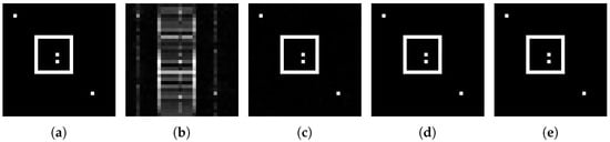
Figure 2. Visual results for Scene 1, a simulated $32\times 32$ scene obtained by various methods. (a) Original. (b) Polar format. (c) SDA. (d) WAMA. (e) CFBA.

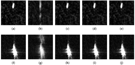
Figure 3. Visual results for Scene 2 (a $64\times 64$ patch from TerraSAR-X) and Scene 3 (a $64\times 64$ patch from Sentinel-1) obtained by various methods. First row for Scene 2, the second row for Scene 3. (a) Original. (b) Polar format. (c) SDA. (d) WAMA. (e) CFBA. (f) Original. (g) Polar format. (h) SDA. (i) WAMA. (j) CFBA.

In the fourth and the fifth experiment, two simulated images of the sea surface were used as the original scene, with the first one only including sea waves, and the second including a travelling ship and its wake as well. Simulated as the scenes are, they are not as simple as Scene 1, which is a mere combination of black and white regions resembling point reflectors, but are rather based on an exquisite model taking the most important SAR imaging effects into account [29]. The scenes are based on a model of the sea surface using the Pierson–Moskowitz spectrum and cosine-squared spreading function with wind speed $V_w=8$ m/s for the first image and $V_w=4$ m/s for the second image, with waves traveling at ${45}^{\circ }$ relative to the SAR flight direction. For the second image, the size of the ship is 55 m, with 8 m beam and 3 m draft, moving at a velocity of 8 m/s at ${45}^{\circ }$ relative to the SAR flight direction. The original size of both SAR images is $1\times 1$ km with a spatial resolution of 1.25 m, while SAR platform parameters are as follows: the platform altitude is 2.5 km, platform velocity is 125 m/s, the incidence angle is ${\theta }_r$ = ${35}^{\circ }$, and signal parameters are X-band (9.65 GHz) and VV polarization. Both scenes shown here are of $128\times 128$ pixels, patches from the original images due to heavy computational burden, and their corresponding corrupted pseudo-phase histories are generated from them in the same way as aforementioned.

The visual results for all 4 methods for the fourth experiment and the fifth experiment are shown in Figure 4 in the first row and the second row, respectively. Since the original pixel values in the images are rather small, for visual convenience, the “imadjust” function in Matlab was used before depicting. For the fourth experiment, the results of SDA, WAMA, and CFBA are with better contrast, i.e., the bright regions in (c), (d), (e) of Figure 4 are brighter than those in (b), and their dark regions are darker. For the fifth experiment, (h), (i), (j) are sharper than (g) and display much more concentrated ship wakes. Meanwhile, the numerical results in Table 2 also demonstrate that CFBA, SDA, and WAMA give comparable performance. In terms of MSE, SDA outperforms WAMA and is outperformed by CFBA. As for entropy values, WAMA is the best.

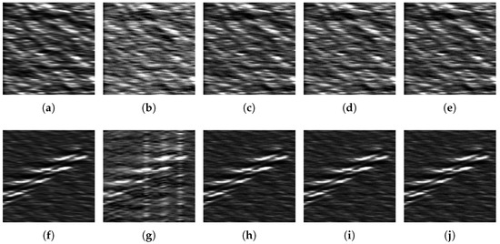
Figure 4. Visual results for Scene 4 and Scene 5, two $128\times 128$ simulated sea surfaces, obtained by various methods. First row for Scene 4, the second row for Scene 5. (a) Original. (b) Polar format. (c) SDA. (d) WAMA. (e) CFBA. (f) Original. (g) Polar format. (h) SDA. (i) WAMA. (j) CFBA.

As for the convergence of CFBA and WAMA, Figure 5 displays how $J({\mathit{f}}^{(n)},{\mathit{\varphi }}^{(n)})$ changes with increasing n until the stopping criterion is satisfied for both the WAMA method and the proposed CFBA method, taking the first three experiments as examples. In each sub-figure, the vertical axis represents $J({\mathit{f}}^{(n)},{\mathit{\varphi }}^{(n)})$, the value of the cost function (7) computed for ${\mathit{f}}^{(n)}$ and ${\mathit{\varphi }}^{(n)}$, while the horizontal axis represents the iterative numbers n in the loop of the alternating minimization. The red line represents the case of WAMA, and the blue line represents the case of CFBA. It can be seen that in all three experiments, $J({\mathit{f}}^{(n)},{\mathit{\varphi }}^{(n)})$ decreases monotonically for both CFBA and WAMA. This is consistent with the conclusions of our convergence analysis, and gives an experimental validation for the convergence of CFBA and WAMA in a sense. Moreover, it can be observed that CFBA converges more rapidly, since it reaches the stopping criterion with fewer iterations.

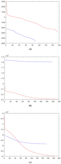
Figure 5. The values of $J(f^{(n)},{\varphi }^{(n)})$ for WAMA (red lines) and CFBA (blue lines) until the stopping criterion was satisfied. (a) Scene 1. (b) Scene 2. (c) Scene 3.

6. Conclusions

In this paper, an optimization solution regularized by the magnitude Cauchy penalty is proposed for the problem of simultaneously reconstructing and autofocusing a SAR image. An alternating minimization framework named CFBA is proposed to solve this inverse problem, in which the sub-problems related to the desired SAR image are solved by a complex forward-backward splitting method, and its convergence is analyzed. Additionally, the WAMA method based on Wirtinger calculus is revisited and further discussed, in particular in respect to its convergence. Experimental results on simulated phase history data derived from several simulated as well as real SAR images of the sea surface demonstrate that the proposed CFBA method can reconstruct highly focused SAR images and effectively remove phase errors, showing performance competitive with that of WAMA. Our current work focuses on the design of SAR autofocusing approaches in the context of compressive data acquisition, and we will aim to address the problem by combining our current model-based techniques with data-driven methods.

References

- Moreira, A.; Prats-Iraola, P.; Younis, M.; Krieger, G.; Hajnsek, I.; Papathanassiou, K.P. A Tutorial on Synthetic Aperture Radar. IEEE Geosci. Remote Sens. Mag. 2013, 1, 6–43. [Google Scholar] [CrossRef] [Green Version]
- Ouchi, K. Recent Trend and Advance of Synthetic Aperture Radar with Selected Topics. Remote Sens. 2013, 5, 716–807. [Google Scholar] [CrossRef] [Green Version]
- Graziano, M.D.; D’Errico, M.; Rufino, G. Wake Component Detection in X-Band SAR Images for Ship Heading and Velocity Estimation. Remote Sens. 2016, 8, 498. [Google Scholar] [CrossRef] [Green Version]
- Wahl, D.E.; Eichel, P.; Ghiglia, D.; Jakowatz, C. Phase Gradient Autofocus - a Robust Tool for High Resolution SAR Phase Correction. IEEE Trans. Aerosp. Electron. Syst. 1994, 30, 827–835. [Google Scholar] [CrossRef] [Green Version]
- Calloway, T.M.; Donohoe, G.W. Subaperture Autofocus for Synthetic Aperture Radar. IEEE Trans. Aerosp. Electron. Syst. 1994, 30, 617–621. [Google Scholar] [CrossRef]
- Tsakalides, P.; Nikias, C. High-resolution Autofocus Techniques for SAR Imaging Based on Fractional Lower-order Statistics. IEE Proc.-Radar Sonar Navig. 2001, 148, 267–276. [Google Scholar] [CrossRef]
- Fienup, J.; Miller, J. Aberration Correction by Maximizing Generalized Sharpness Metrics. J. Opt. Soc. Am. A 2003, 20, 609–620. [Google Scholar] [CrossRef]
- Morrison, R.L.; Do, M.N.; Munson, D.C. SAR Image Autofocus by Sharpness Optimization: A Theoretical Study. IEEE Trans. Image Process. 2007, 16, 2309–2321. [Google Scholar] [CrossRef]
- Kragh, T.J.; Kharbouch, A.A. Monotonic Iterative Algorithm for Minimum-entropy Autofocus. Adapt. Sens. Array Process. Workshop 2006, 40, 1147–1159. [Google Scholar]
- Zeng, T.; Wang, R.; Li, F. SAR Image Autofocus Utilizing Minimum-entropy Criterion. IEEE Geosci. Remote Sens. Lett. 2013, 10, 1552–1556. [Google Scholar] [CrossRef]
- Kantor, J.M. Minimum Entropy Autofocus Correction of Residual Range Cell Migration. In Proceedings of the 2017 IEEE Radar Conference (RadarConf), Seattle, WA, USA, 8–12 May 2017; pp. 0011–0016. [Google Scholar]
- Onhon, N.Ö.; Cetin, M. A Sparsity-driven Approach for Joint SAR Imaging and Phase Error Correction. IEEE Trans. Image Process. 2011, 21, 2075–2088. [Google Scholar] [CrossRef]
- Kelly, S.I.; Yaghoobi, M.; Davies, M.E. Auto-focus for Under-sampled Synthetic Aperture Radar. In Proceedings of the Sensor Signal Processing for Defence (SSPD 2012), London, UK, 25–27 September 2012. [Google Scholar]
- Kelly, S.; Yaghoobi, M.; Davies, M. Sparsity-based Autofocus for Undersampled Synthetic Aperture Radar. IEEE Trans. Aerosp. Electron. Syst. 2014, 50, 972–986. [Google Scholar] [CrossRef] [Green Version]
- Güngör, A.; Cetin, M.; Güven, H.E. An Augmented Lagrangian Method for Autofocused Compressed SAR Imaging. In Proceedings of the 2015 3rd International Workshop on Compressed Sensing Theory and Its Applications to Radar, Sonar and Remote Sensing (CoSeRa), Pisa, Italy, 17–19 June 2015; pp. 1–5. [Google Scholar]
- Güngör, A.; Çetin, M.; Güven, H.E. Autofocused Compressive SAR Imaging Based on the Alternating Direction Method of Multipliers. In Proceedings of the 2017 IEEE Radar Conference (RadarConf), Seattle, WA, USA, 8–12 May 2017; pp. 1573–1576. [Google Scholar]
- Uḡur, S.; Arıkan, O. SAR Image Reconstruction and Autofocus by Compressed Sensing. Digit. Signal Process. 2012, 22, 923–932. [Google Scholar] [CrossRef]
- Ash, J.N. An Autofocus Method for Backprojection Imagery in Synthetic Aperture Radar. IEEE Geosci. Remote Sens. Lett. 2011, 9, 104–108. [Google Scholar] [CrossRef]
- Sommer, A.; Ostermann, J. Backprojection Subimage Autofocus of Moving Ships for Synthetic Aperture Radar. IEEE Trans. Geosci. Remote Sens. 2019, 57, 8383–8393. [Google Scholar] [CrossRef]
- Kantor, J.M. Polar Format-Based Compressive SAR Image Reconstruction With Integrated Autofocus. IEEE Trans. Geosci. Remote Sens. 2019, 58, 3458–3468. [Google Scholar] [CrossRef]
- Mason, E.; Yonel, B.; Yazici, B. Deep learning for SAR image formation. In Algorithms for Synthetic Aperture Radar Imagery XXIV; International Society for Optics and Photonics: San Diego, CA, USA, 2017; Volume 10201, p. 1020104. [Google Scholar]
- Pu, W. Deep SAR Imaging and Motion Compensation. IEEE Trans. Image Process. 2021, 30, 2232–2247. [Google Scholar] [CrossRef]
- Brandwood, D. A Complex Gradient Operator and its Application in Adaptive Array Theory. IEE Proc. H (Microw. Opt. Antennas) 1983, 130, 11–16. [Google Scholar] [CrossRef]
- Van Den Bos, A. Complex Gradient and Hessian. IEE Proc.-Vis. Image Signal Process. 1994, 141, 380–382. [Google Scholar] [CrossRef]
- Kreutz-Delgado, K. The Complex Gradient Operator and the CR-calculus. arXiv 2009, arXiv:0906.4835. [Google Scholar]
- Bouboulis, P. Wirtinger’s Calculus in General Hilbert Spaces. arXiv 2010, arXiv:1005.5170. [Google Scholar]
- Zhang, Z.Y.; Pappas, O.; Achim, A. SAR Image Autofocusing using Wirtinger calculus and Cauchy regularization. In Proceedings of the ICASSP 2021—2021 IEEE International Conference on Acoustics, Speech and Signal Processing (ICASSP), Toronto, ON, Canada, 6–11 June 2021; pp. 1455–1459. [Google Scholar]
- Pappas, O.; Achim, A.; Bull, D. Superpixel-level CFAR detectors for ship detection in SAR imagery. IEEE Geosci. Remote Sens. Lett. 2018, 15, 1397–1401. [Google Scholar] [CrossRef] [Green Version]
- Rizaev, I.G.; Karakuş, O.; Hogan, S.J.; Achim, A. Modeling and SAR Imaging of the Sea Surface: A Review of the State-of-the-Art with Simulations. ISPRS J. Photogramm. Remote Sens. 2022, 187, 120–140. [Google Scholar] [CrossRef]
- Çetin, M.; Karl, W.C. Feature-enhanced synthetic aperture radar image formation based on nonquadratic regularization. IEEE Trans. Image Process. 2001, 10, 623–631. [Google Scholar] [CrossRef] [PubMed] [Green Version]
- Carrara, W.; Goodman, R.S.; Majewski, R.M. Spotlight Synthetic Aperture Radar: Signal Processing Algorithms; Artech House: Norwood, MA, USA, 1995. [Google Scholar]
- McCullagh, P.; Polson, N.G. Statistical Sparsity. Biometrika 2018, 105, 797–814. [Google Scholar] [CrossRef]
- Karakuş, O.; Achim, A. On Solving SAR Imaging Inverse Problems Using Non-convex Regularization with a Cauchy-Based Penalty. IEEE Trans. Geosci. Remote Sens. 2021, 59, 5828–5840. [Google Scholar] [CrossRef]
- Karakuş, O.; Mayo, P.; Achim, A. Convergence Guarantees for Non-convex Optimisation with Cauchy-based Penalties. IEEE Trans. Signal Process. 2020, 68, 6159–6170. [Google Scholar] [CrossRef]
- Soulez, F.; Thiébaut, É.; Schutz, A.; Ferrari, A.; Courbin, F.; Unser, M. Proximity Operators for Phase Retrieval. Appl. Opt. 2016, 55, 7412–7421. [Google Scholar] [CrossRef] [Green Version]
- Güven, H.E.; Güngör, A.; Cetin, M. An Augmented Lagrangian Method for Complex-valued Compressed SAR Imaging. IEEE Trans. Comput. Imaging 2016, 2, 235–250. [Google Scholar] [CrossRef]
- Attouch, H.; Bolte, J.; Redont, P.; Soubeyran, A. Proximal Alternating Minimization and Projection Methods for Nonconvex Problems: An Approach Based on the Kurdyka-Łojasiewicz Inequality. Math. Oper. Res. 2010, 35, 438–457. [Google Scholar] [CrossRef] [Green Version]
- Attouch, H.; Bolte, J.; Svaiter, B.F. Convergence of Descent Methods for Semi-algebraic and Tame Problems: Proximal Algorithms, Forward–backward Splitting, and Regularized Gauss–Seidel Methods. Math. Program. 2013, 137, 91–129. [Google Scholar] [CrossRef]
- Csiszár, I. Information Geometry and Alternating Minimization Procedures. Stat. Decis. 1984, 1, 205–237. [Google Scholar]
- Byrne, C.L. Alternating Minimization as Sequential Unconstrained Minimization: A Survey. J. Optim. Theory Appl. 2013, 156, 554–566. [Google Scholar] [CrossRef]
- Barrett, R.; Berry, M.; Chan, T.F.; Demmel, J.; Donato, J.; Dongarra, J.; Eijkhout, V.; Pozo, R.; Romine, C.; Van der Vorst, H. Templates for the Solution of Linear Systems: Building Blocks for Iterative Methods; SIAM Press: Philadelphia, PA, USA, 1994. [Google Scholar]
- Florescu, A.; Chouzenoux, E.; Pesquet, J.C.; Ciuciu, P.; Ciochina, S. A Majorize-minimize Memory Gradient Method for Complex-valued Inverse Problems. Signal Process. 2014, 103, 285–295. [Google Scholar] [CrossRef] [Green Version]
- Çetin, M.; Karl, W.C.; Willsky, A.S. Feature-preserving Regularization Method for Complex-valued Inverse Problems with Application to Coherent Imaging. Opt. Eng. 2006, 45, 017003. [Google Scholar]
- Geman, D.; Reynolds, G. Constrained Restoration and the Recovery of Discontinuities. IEEE Trans. Pattern Anal. Mach. Intell. 1992, 14, 367–383. [Google Scholar] [CrossRef]
- Joly, P.; Meurant, G. Complex Conjugate Gradient Methods. Numer. Algorithms 1993, 4, 379–406. [Google Scholar] [CrossRef]
- Walker, J.L. Range-Doppler Imaging of Rotating Objects. IEEE Trans. Aerosp. Electron. Syst. 1980, AES-16, 23–52. [Google Scholar] [CrossRef]
- Krantz, S.G.; Parks, H.R. A Primer of Real Analytic Functions; Springer Science & Business Media: Berlin/Heidelberg, Germany, 2002. [Google Scholar]
- Zhang, S.; Xia, Y.; Zheng, W. A Complex-valued Neural Dynamical Optimization Approach and its Stability Analysis. Neural Netw. 2015, 61, 59–67. [Google Scholar] [CrossRef]
- Liu, S.; Jiang, H.; Zhang, L.; Mei, X. A Neurodynamic Optimization Approach for Complex-variables Programming Problem. Neural Netw. 2020, 129, 280–287. [Google Scholar] [CrossRef]
Publisher’s Note: MDPI stays neutral with regard to jurisdictional claims in published maps and institutional affiliations. |
© 2022 by the authors. Licensee MDPI, Basel, Switzerland. This article is an open access article distributed under the terms and conditions of the Creative Commons Attribution (CC BY) license (https://creativecommons.org/licenses/by/4.0/).