Fusing Spatial Attention with Spectral-Channel Attention Mechanism for Hyperspectral Image Classification via Encoder–Decoder Networks

Abstract

In recent years, convolutional neural networks (CNNs) have been widely used in hyperspectral image (HSI) classification. However, feature extraction on hyperspectral data still faces numerous challenges. Existing methods cannot extract spatial and spectral-channel contextual information in a targeted manner. In this paper, we propose an encoder–decoder network that fuses spatial attention and spectral-channel attention for HSI classification from three public HSI datasets to tackle these issues. In terms of feature information fusion, a multi-source attention mechanism including spatial and spectral-channel attention is proposed to encode the spatial and spectral multi-channels contextual information. Moreover, three fusion strategies are proposed to effectively utilize spatial and spectral-channel attention. They are direct aggregation, aggregation on feature space, and Hadamard product. In terms of network development, an encoder–decoder framework is employed for hyperspectral image classification. The encoder is a hierarchical transformer pipeline that can extract long-range context information. Both shallow local features and rich global semantic information are encoded through hierarchical feature expressions. The decoder consists of suitable upsampling, skip connection, and convolution blocks, which fuse multi-scale features efficiently. Compared with other state-of-the-art methods, our approach has greater performance in hyperspectral image classification.

1. Introduction

Hyperspectral imaging (HSI) is a technique for analyzing wide spectrum light that yields a wide range of spectral information about the Earth’s surface [1]. They are widely used in various surface monitoring fields, such as geology, agriculture, forestry, and the environment [2,3,4]. An essential challenge in hyperspectral remote sensing (HRS) is the classification of hyperspectral image (HSI), which assigns each pixel a unique semantic label [5].

The traditional methods use machine learning-based classifiers to classify hyperspectral images. These traditional classifiers work for HSI classification, such as random forest (RF) [6], support vector machine (SVM) [7], canonical correlation forest (CCF) [8,9], multinomial logistic regression (MLR) [10], and rotation forest (RoF) [11]. These methods first extract the features and then classify hyperspectral images through some designed classifiers. In the initial research, researchers only consider spectral information in hyperspectral images, however, these are lacking effective feature encoding means. Follow-up research has indicated that the spatial contextual information of hyperspectral images plays a significant role in the classification of HSI. Therefore, the researchers integrated the extraction of spatial information into the existing pipeline [12,13,14].

The hyperspectral image classification task has used deep learning methods [15,16,17,18] and achieved impressive results in recent years. Researchers apply some excellent deep learning algorithms in computer vision to hyperspectral images [19], such as convolutional neural network (CNN) [17,20], 3D convolutional neural network(3D-CNN), recurrent neural network (RNN) [21,22], and multi-scale convolutional neural networks [21,23]. Wu et al. [24] propose to use RNN for modeling the dependencies between different spectral bands and then use a convolutional recurrent neural network (CRNN) to learn more discriminative features for hyperspectral image classification. Lee et al. [25] propose a deeper neural network to explore local contextual information for hyperspectral image classification.

In recent years, some CNN-based approaches [26,27,28] were proposed to promote the performance of HSI classification. The research found that CNN-based classifiers [25,29] can improve the ability to extract spectral–spatial contextual information from hyperspectral images. Feng et al. [29] propose a semi-supervised approach to explore spectral geometry and spatial geometric structure information. These approaches generally decompose hyperspectral pictures into $s\times s$-sized chunks before applying CNN classifiers on each block, called a patch-based local learning framework. Due to the limitation of convolutional receptive fields, convolutional neural networks have difficulty in modeling global spatial information, which hinders the accurate classification of each pixel of hyperspectral images. Shen et al. [30] propose various non-local modules to be used to efficiently aggregate the correspondence of each pixel with all other pixels. ENL-FCN [30] explores non-local spatial information in a criss-cross way which limits the utilization of spectral channel information. However, these CNN-based methods are insufficient to simultaneously encode features for spatial and spectral channels in hyperspectral images. On the one hand, the deep spatial–spectral information of hyperspectral images is difficult to describe and extract simply. On the other hand, CNNs extract features by local convolutional operations. Large convolutional kernels lose local details, and small convolutional kernels lack a global view. Therefore, the existing methods cannot simultaneously model spatial context information and spectral channel information in a targeted manner.

To this end, we proposed an encoder–decoder pipeline based on the multi-source fusion attention mechanism. The multi-source fusion attention mechanism, which consists of the spatial and spectral attention modules, was proposed to encode long-range contextual information and mine spectral channel features. Specifically, the spatial attention module encoded local–global spatial contextual information. The spectral attention module was used to pay attention to the representative spectral channels in the classification. Meanwhile, we proposed three fusion methods to fuse spatial and spectral attention effectively: (1) we directly add the obtained spatial and spectral attention scores; (2) we concatenate on the obtained spatial attention feature map and the spectral attention feature map in the dimension of the channel, and then we use a multilayer perceptron (MLP) [31]; (3) we apply the Hadamard product between the spatial attention matrix and spectral attention matrix with values (V). To produce an exchange of information between different windows in a hyperspectral image, we proposed the encoder transformer block based on a multi-source fusion attention mechanism as the basic feature learning unit. Each transformer block consists of four parts: LayerNorm (LN) layer, multi-source fusion attention mechanism, residual connection, and MLP. The encoder transformer block is used in the encoder section which consists of two successive transformer blocks. The output of the previous block was used as an input to the next block. We used a hierarchical transformer framework based on transformer blocks as an encoder to generate hierarchical feature representations such as CNN. The encoder was able to acquire features at different scales with the powerful global modeling capability of the transformer. In the decoder, we employ bilinear interpolation to perform the upsampling operation to restore the spatial resolution of the feature maps. We use skip connections and convolution blocks to establish the global dependencies between the features at different scales.

The main contributions of this article can be summarized as follows:

• To better encode the rich spectral–spatial information of the hyperspectral image, we propose a multi-source fusion attention mechanism. The multi-source fusion attention mechanism can consider the spectral channels and the spatial attention, which can help the network achieve better classification.
• To encode long-range contextual information, we propose our encoder by combining the advantages of a hierarchical transformer. In the encoder, the transformer block and the hierarchical transformer architecture have powerful feature extraction capabilities, which can obtain both shallow local features and high-level global rich semantic information.
• We propose an encoder–decoder transformer framework for hyperspectral image classification. By integrating the multi-source fusion attention mechanism with the transformer framework, our framework can effectively extract and utilize the spectral–spatial information of the hyperspectral images.

The rest of this paper is planned as follows. Section 2 briefly introduces the related work. Section 3 describes our proposed method. Section 4 contains an analysis of the experiments and results of our method on the datasets. The ablation study is discussed in Section 5. Finally, Section 6 concludes this paper.

2. Related Work

2.1. CNN-Based Methods

The convolutional neural networks (CNNs) are the mainstream methods for hyperspectral image (HSI) classification. In [32], they propose a method to encode spatial and spectral information directly using 2D convolutional neural networks (2D-CNN) and use a multilayer perceptron for the final classification. Li et al. [33] view HSI as a voxel. They propose to use 3D convolutional neural networks (3D-CNN) to extract spectral–spatial information. Zhong et al. [34] propose the spectral–spatial residual network (SSRN), which introduced residual links in 3D-convolutional layers to help learn spectral and spatial features. Ma et al. [35] propose a double-branch multi-attention mechanism (DBMA), which uses two sub-networks to extract spectral and spatial features, respectively, and introduces two attention mechanisms. Despite the fact that standard CNN-based classification methods have achieved high classification accuracy, they are unable to model long-range contextual information. The main reason is that these methods are patch-based frameworks rather than working directly on the whole image [16,17,25,36,37].

2.2. FCN-Based Methods

Research has shown that fully convolutional neural networks (FCN) have excellent performance in computer vision. Unlike the patch-based CNN approaches, U-Net [38] uses the whole HSI input to extract high-dimensional features then extend to their original dimensions for eventual pixel-level classification. Zheng et al. [39] propose an encoder–decoder FCN, using the whole image as input to extract global spatial information. It is termed the patch-free global learning framework (FPGA). It employs a global stochastic stratification (GS2) sampling approach to obtain diverse gradients and ensure FCN convergence in the FPGA framework. However, when the sample data is unbalanced, it is difficult for the FPGA to extract the most valuable features. In response to the problem of unbalanced classification samples, Zhu et al. [40] propose a spectral–spatial-dependent global learning framework based on global convolutional long short-term memory and global joint attention mechanism. FCN uses the whole image as input to encode global features favorably but lacks attention to local features. Shen et al. [30] propose introducing non-local modules into FCN to combine long-range context information. In our method, we adopted an FCN-based transformer architecture to develop our encoder to achieve a situation where local and global spatial information can be considered in the HSI classification task.

2.3. Transformer-Based Methods

The transformer [41] has made significant progress in natural language processing. Inspired by the transformer, transformer-based methods are being used in computer vision (CV) tasks [42]. ViT [43] is the first attempt to apply the transformer to a vision task which has achieved very good results in ImageNet image classification. However, it often needs to be trained on big data to perform well. Deit [44] introduces several training strategies into ViT that allow the vision transformer to perform well on small datasets. Recently, there has been a lot of work on vision transformers [45,46,47]. Among these, the work of the swin transformer [45], a creative hierarchical vision transformer, is capable of serving as a backbone for computer vision. The swin transformer [45] generates the hierarchical architectures through patch merging operations to allow flexible modeling. With a creative shift mechanism, the hierarchical architecture has the complexity of a linear calculation of the image size. The powerful capabilities of the swin transformer [45] make it compatible with vision tasks surpassing the previous state-of-the-art methods. The transformer performs well on computer vision tasks, but lacks exploration in hyperspectral images. Motivated by the great potential of the swin transformer, we propose a transformer architecture based on the multi-source fusion attention mechanism, which uses a hierarchical transformer as the encoder to extract the global spatial context information and spectral features of hyperspectral images. Unlike traditional transformers applied to natural images, we try to explore the applied potential of the transformer framework in HSI classification.

3. Proposed Method

In order to extract the spatial contextual information among all pixels as well as to notice discriminative spectral channels, we proposed an encoder–decoder network that fuses local–global spatial attention and spectral-channel attention for hyperspectral image (HSI) classification. The overall network architecture is shown in Figure 1; the whole hyperspectral image is used as the input, where H, W, and channel represent the height, width, and number of spectral bands, respectively. The details of each part are described in the following subsections.

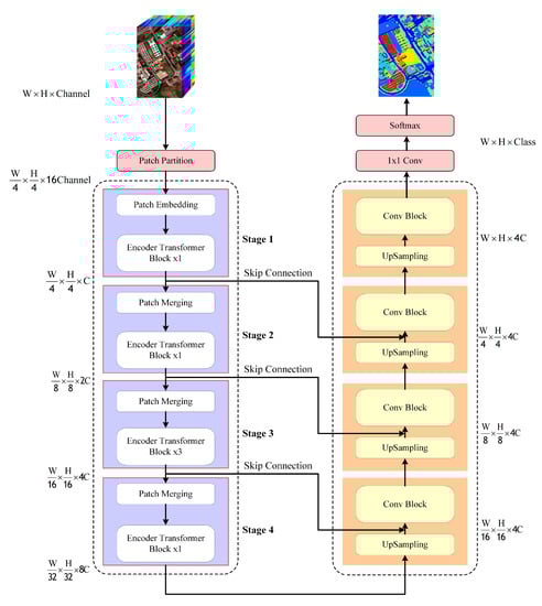
Figure 1. Flowchart of proposed HSI classification framework.

3.1. Multi-Source Fusion Attention Mechanism

The multi-source fusion attention mechanism consists of the spatial attention module and the spectral-channel attention module. Each pixel in a hyperspectral image is associated with pixels in adjacent local regions, as well as with long-range contextual information in the entire image. Therefore, encoding long-range spatial contextual information will increase the accuracy of the hyperspectral image classification. The spatial attention module is used for encoding hyperspectral image spatial contextual information. Each spectral channel in a hyperspectral image has its own importance; therefore, feature encoding also needs to consider spectral contextual information. Unlike the spatial attention, the significance of the spectral-channel attention module is in modeling the channel information, which is used to find significant channels for a feature detector.

The spatial attention module is shown in Figure 2a; similar to the swin transformer [45], the input features X are mapped through the linear layer to learn the relationship query (Q), key (K) between pixels, and extract feature value (V). The Q and K are learned pixel-to-pixel relationships, including spatial and spectral, and learned attention relation is applied to the feature V through matrix computation. The dimension of Q and K and V is $N\times C$, where N is the number of patches in a spatial, and C is the number of spectral channel dimension. In our spatial attention module, we first obtain the transpose matrix of $K^{N\times C}$, then multiply $Q^{N\times C}$ by $K^T$ and divide by $\sqrt{C}$. Based on the swin transformer [45], we also follow [31,48,49,50] to include a relative position bias (b) where $B\in R^{N\times N}$. Spatial feature maps of shape $N\times N$ are fed to the softmax function for learning the spatial attention matrix. Finally, we multiply the output with value to map the spatial attention to the input features. The spatial attention equation (${\mathrm{A}}_{\mathrm{spatial}}$) is expressed as follows:

$$\mathrm{A}{}_{\mathrm{spatial}}=SoftMax\left(\frac{Q·K^T}{\sqrt{C}}+B\right)·V$$

(1)

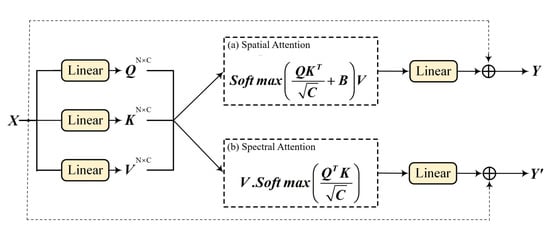
Figure 2. Attention mechanisms.

Figure 3a visualizes the spatial local-global correlations of hyperspectral image tokens. The spatial attention method can help the network learn the local and global spatial contextual information. Therefore, hyperspectral image local and global spatial information can be used effectively.

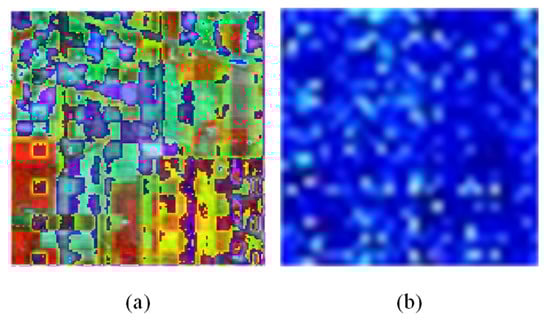
Figure 3. Heatmap for the attention matrix: (a) spatial attention heatmap; (b) spectral-channel attention heatmap.

The spectral-channel attention module is shown in Figure 2b. Different from the swin transformer [45], we first obtain the transposed matrix of $Q^{N\times C}$, then multiply it by $K^{N\times C}$ and divide by $\sqrt{C}$ and obtain a spectral channel attention matrix by softmax; the shape is $C\times C$. Then, we multiply the value with the output to map the spectral channel attention to the input features. We computed the spectral-channel attention equation ($\mathrm{A}{}_{\mathrm{spectral}}$) as follows:

$$\mathrm{A}{}_{\mathrm{spectral}}=V·SoftMax\left(\frac{Q^T·K}{\sqrt{C}}\right)$$

(2)

Figure 3b shows the visualization of the spatial-channel attention feature map; it helps the neural network to focus on those spectral channels of interest.

Unlike DBMA [35], the computation of our spatial- and spectral-channel attention matrices takes the same input and is obtained through the operation of the matrices. Our method has higher efficiency and less computational overhead.

We propose three ways to fuse spatial attention and spectral-channel attention effectively. (1) Figure 4a shows that the shape of the output features after performing spatial attention and spectral channel attention is the same; we use matrix addition for fusion, which can be expressed as Equation (3). (2) As shown in Figure 4b, we concatenate the obtained spatial attention feature map and spectral channel attention feature map in the dimension of the channel. Then we use a multi-layer perceptron (MLP) [51], which can be expressed as Equation (4). (3) Figure 4c shows that we apply the Hadamard product between the spatial attention matrix and the spectral-channel attention matrix, which can be expressed as Equation (5).

$$\mathrm{A}{}_{add}=SoftMax\left(\frac{Q·K^T}{\sqrt{C}}+B\right)·V+V·SoftMax\left(\frac{Q^T·K}{\sqrt{C}}\right)$$

(3)

$$\mathrm{A}{}_{\mathrm{cat}}=MLP\left\{\mathrm{cat}\left(\mathrm{SoftMax}\left(\frac{Q·K^T}{\sqrt{C}}+B\right)·V,V·SoftMax\left(\frac{Q^T·K}{\sqrt{C}}\right)\right)\right\}$$

(4)

$$\mathrm{A}{}_{mul}=SoftMax\left(\frac{Q·K^T}{\sqrt{C}}+B\right)·V·SoftMax\left(\frac{Q^T·K}{\sqrt{C}}\right).$$

(5)

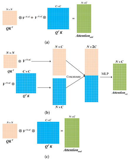
Figure 4. The three types of attention fusion: (a) add; (b) concatenate; (c) multiply.

In our experiments (discussed in Section 5), the multi-source fusion attention mechanism, which fuses spatial attention with spectral-channel attention, can achieve a better classification performance in HSI.

3.2. Framework

Inspired by the swin transformer [45], we propose our encoder–decoder transformer framework based on a multi-source fusion attention mechanism.

3.2.1. Encoder

In the encoder part, we use two successive transformer blocks, the window-based multi-source fusion attention module (W-FA) and the shifted window-based multi-source fusion attention module (SW-FA), as encoder transformer blocks. Figure 5 shows the two successive blocks structure in detail.

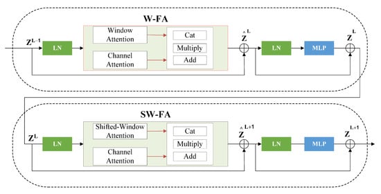
Figure 5. Encoder transformer block.

In the encoder transformer block, the output feature $Z^{L-1}$ of the previous block is used as the input of the current block. The $Z^{L-1}$ applys the linear normalization (LN) and input to W-FA. The windows attention is the spatial attention operation we mentioned above. The channel attention operates as described in Equation (2), and the output of the W-FA is obtained through the fusion mechanism. The output of the W-FA performs a residual connection with $Z^{L-1}$ to obtain ${\widehat{Z}}^L$. Then, after another linear normalization, MLP and residual connection are used to obtain $Z^L$. The problem with the W-FA is that there is no interaction between the different windows, which limits global information interactions. Therefore, we follow the shifted-window attention mechanism in the swin transformer [45], adding spectral channel attention proposed in the SW-FA to achieve spatial and spectral channel information interactions across the windows. Similar to W-FA, $Z^L$ is the input to SW-FA after a linear normalization and it performs a residual connection to obtain ${\widehat{Z}}^{L+1}$. Finally, after another linear normalization, MLP and residual connection are used to obtain the $Z^{L+1}$ of encoder transformer block output. This process can be formulated as follows:

$$\begin{array}{c}{\widehat{z}}_L=W-FA\left(LN\left(z_{L-1}\right)\right)+z_{L-1}\\ z_L=MLP\left(LN\left({\widehat{z}}_L\right)\right)+z_L\end{array}$$

(6)

$$\begin{array}{cc}\hfill & {\widehat{z}}_{L+1}=SW-FA\left(LN\left(z_L\right)\right)+z_L\hfill \\ \hfill & z_{L+1}=MLP\left(LN\left({\widehat{z}}_{L+1}\right)\right)+z_{L+1}\hfill \end{array}$$

(7)

SW-FA differs from the previous W-FA in that SW-FA is an efficient cyclic-shifting operating [45] without additional calculations. Based on the shift window mechanism, it can generate information interactions between windows.

Based on the encoder transformer block, we propose our encoder pipeline. First, we divide the input HSI into non-overlapping windows, and each window patch size is $S\times S$ (set to 4 by default), which generates $\frac{H}{S}\times \frac{W}{S}$ patches, (shown in Figure 6a). The feature size of a patch is $4\times 4\times channel$; its features are treated as a concatenation of raw pixel HIS values. We then map these patches to a predefined dimension C (set to 96) by means of a linear layer. In stage 1, we take these patches as the input to the encoder transformer block. The number of patch ($\frac{H}{4}\times \frac{W}{4}$) remains the same. In stage 2, we performed a patch merging operation [45] to merge $2\times 2$ patches into one, (shown in Figure 6b). The number of patches is changed to $\frac{H}{8}\times \frac{W}{8}$, and the feature dimension is changed from C to 4C. These merged features are the input into the second encoder transformer block, and the output dimension is set to 2C. A $2\times downsampling$ was achieved in this process. The number of patches is cut down by patch merging, thereby generating hierarchical representations at different network depths. In stages 3 and 4, as the number of patches is reduced and channel dimensions increased, we increase the number of transformer blocks used for feature encoding. As shown in Figure 1 left, to balance the depth of the network and the complexity of the model, the number of transformer blocks for each of the four stages is set to $=\{1,1,3,1\}$. The encoder can obtain deep features and hierarchical representations by downsampling from four stages. The output resolution of the encoder transformer block in each stage is $\frac{H}{4}\times \frac{W}{4}$, $\frac{H}{8}\times \frac{W}{8}$, $\frac{H}{16}\times \frac{W}{16}$, $\frac{H}{32}\times \frac{W}{32}$, respectively. In the first and second stages of encoding, it is used to learn shallow local features, and in the subsequent encoding stages, it is used to learn deep global features.

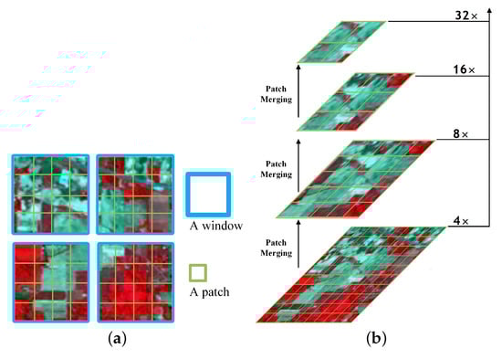
Figure 6. (a) Window partitioning. (b) Patch merging.

3.2.2. Decoder

As shown in Figure 1 right, the decoder consists of four stages. Each stage includes upsample (bilinear interpolation), skip connections, and convolution block. The conv block consists of the $3\times 3$ convolutional, followed by the group normalization layer and ReLU activation function. Specifically, the output of stage 4 in the encoder is used as the initial input of the decoder. The input features are upsampled by $\times 2$, and the shape changes from $\frac{H}{32}\times \frac{W}{32}\times 8C$ to $\frac{H}{16}\times \frac{W}{16}\times 4C$. In order to preserve the shallow hierarchical representation and prevent the loss of features, we used skip connections, i.e., adding the output of the encoder stage (shaped similar to $\frac{H}{16}\times \frac{W}{16}\times 4C$) with the upsampled features. Its operation is similar to the lateral connections of the feature pyramid network [52]. In this way, we fused features from different scales from the encoder during decoding. To keep the channel dimensions of the multi-scale feature maps in skip connections consistent with the upsampled feature maps, we used linear layers to keep the dimensions consistent. At the end of the decoder, $1\times 1$ convolution and softmax are used to map the final feature map to each class. In our encoder, the low-stage output feature maps are rich in global information, and the high-stage output feature maps which contain more are rich in semantic details and local information. Our decoder structure can effectively fuse different stage output feature maps in the encoder.

4. Experimental Results and Analysis

4.1. Experimental Settings

4.1.1. Model Parameters

The entire HSI needs to be divided into non-overlapping patches before being input to the encoder transformer block; we expanded the dimension of the input image to a multiple of the patch size (default is four). For this operation, we used the zero-fill method. The channel number of the hidden layers in the first stage was set to 96 and the layer numbers were set to $=\{2,2,6,2\}$.

4.1.2. Optimized Parameters

The number of learning iterations was 200. We used Adam to minimize the classification cross-entropy loss. The learning rate was set to 0.0004. The momentum was set to 0.9 and the decay rate was set to 0.0002.

4.1.3. Metrics

We evaluated our proposed approach quantitatively using four commonly used evaluation metrics to compare with other works. There is the accuracy of each class, the overall accuracy (OA), the average accuracy (AA), and the kappa coefficient (kappa).

4.2. Experiment 1: Kennedy Space Center

The Kennedy Space Center (KSC) dataset was acquired in 1996 by the AVIRIS sensor over the Kennedy Space Center in Florida. This dataset contains $512\times 614$ pixels, with 224 spectral bands. The spatial resolution is about 18 m per pixel. Removing other noise and interference bands, 176 bands of the data were reserved. The KSC dataset includes 13 landcover classes. Figure 7 shows the ground truth, KSC image legend, and the KSC image composed of the three-band false color. Figure 8a–h elucidate the classification outcomes using 2D-CNN [32], 3D-CNN [33], SSRN [34], PyraCNN [53], HybirdSN [54], FCN-CRF [36], ENL-FCN [30], and our proposed method. As seen in the figure, most of our classification results are presented in more giant blobs. It indicates that the same type of ground targets appear in contiguous pieces, which are not single individuals. This is consistent with the fact that manifesting our method has strong robustness when confronted with complex terrestrial hyperspectral image classifications. Table 1 lists the quantity of training and testing data per class. A total of $5\%$ of the data were used as training samples, and the remaining data were tested to assess the model accuracy.

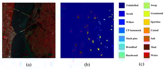
Figure 7. The Kennedy Space Center dataset. (a) Three-band false color composite. (b) Ground-truth map. (c) Legend.

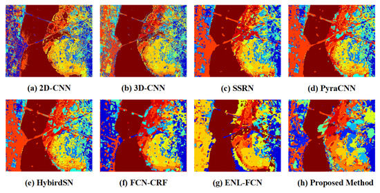
Figure 8. Visualization of the classification maps for the Kennedy Space Center dataset.

Table 1. The amount of training, as well as testing, samples for the Kennedy Space Center dataset.

No.	Land Cover Class	Training	Testing	Total
1	Scrub	18	329	347
2	Willow swamp	13	230	243
3	CP hammock	13	243	256
4	Slash pine	13	239	252
5	Oak/broadleaf	9	152	161
6	Hardwood	12	217	229
7	Swamp	6	99	105
8	Graminoid marsh	20	370	390
9	Spartina marsh	26	494	520
10	Cattail marsh	21	383	404
11	Salt marsh	21	398	419
12	Mud flats	26	477	503
13	Water	47	880	927
	Total	245	4511	4756

In order to quantitatively verify the results, the overall accuracies (OA), the average accuracy (AA), kappa coefficients, and the accuracy of each class are presented in Table 2 for all classification methods (2D-CNN [32], 3D-CNN [33], SSRN [34], PyraCNN [53], HybirdSN [54], FCN-CRF [36], and ENL-FCN [30]). The best accuracy is highlighted in bold.

Table 2. The classification results of 2D-CNN, 3D-CNN, SSRN, PyraCNN, HybirdSN, FCN-CRF, ENL-FCN, and the proposed method on the Kennedy Space Center dataset with $5\%$ labeled samples.

Class	2D-CNN	3D-CNN	SSRN	PyraCNN	HybridSN	FCN-CRF	ENL-FCN	Proposed (add)	Proposed (cat)	Proposed (mul)
1	97.65	88.58	98.84	98.93	98.47	100	99.62	100	100	100
2	88.78	82.31	97.07	92.54	93.75	99.34	100	98.25	100	97.38
3	64.38	73.55	97.13	95.12	89.08	99.17	99.59	100	100	100
4	67.29	60.33	89.77	81.55	89.93	71.94	98.10	100	100	100
5	65.42	64.64	87.78	81.30	90.48	68.33	100	100	100	100
6	79.15	79.29	99.32	89.86	92.98	99.30	100	100	100	100
7	80.14	77.98	93.55	95.27	91.07	33.16	100	100	100	100
8	88.49	93.37	98.59	99.28	93.59	99.01	100	100	99.75	100
9	90.87	88.06	98.50	99.76	94.12	100	100	100	100	98.78
10	99.52	98.36	99.32	99.09	98.36	100	99.93	100	100	100
11	99.64	99.69	99.74	99.97	97.69	100	100	100	100	100
12	97.98	89.44	98.16	99.46	99.19	99.36	96.18	99.79	100	100
13	98.98	98.56	100	100	99.47	100	100	100	100	100
OA	91.06	89.98	97.88	97.04	96.04	96.08	99.46	99.90	99.98	99.75
AA	86.02	84.93	96.75	94.78	94.47	89.97	99.49	99.85	99.98	99.70
kappa	90.04	88.84	97.64	96.70	95.59	95.64	99.40	99.89	99.98	99.73

As shown in Table 2, our proposed method outperforms the previous SOTA ENL-FCN [30] by an improvement of $0.52\%$, $0.49\%$, and $0.58\%$ in terms of OA, AA, and kappa. KSC has the highest spatial resolution in the three experimental datasets, so spatial context information is essential for the classification. From Table 2, we can observe that our proposed method can classify 13 landcover classes with very high accuracy for a training sample proportion of 5 percent. The reason is that the transformer architecture we use effectively establishes global contextual information for high-spatial-resolution images. The classification of each pixel point takes into account other pixels’ spatial information. This demonstrates the robustness of our proposed method in terms of global spatial contextual information. All three proposed fusion methods show excellent classification results.

4.3. Experiment 2: Pavia University

The Pavia University dataset is a hyperspectral image dataset. The image of the dataset consists of $610\times 340$ pixels with 115 spectral bands; we used 103 bands, excluding noise and water absorption regions. The images are divided into 9 categories with a total of 42,776 labeled samples, where the background is removed. Figure 9 shows the Pavia University dataset. Figure 10a–h elucidate the classification outcomes using 2D-CNN [32], 3D-CNN [33], SSRN [34], PyraCNN [53], HybirdSN [54], FCN-CRF [36], ENL-FCN [30], and our proposed method. Table 3 lists the quantity of training and testing data per class. A total of $1\%$ of the data were used as training samples, and the remaining data were tested to assess the model accuracy.

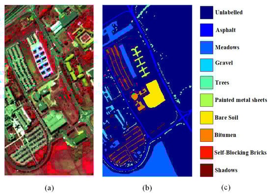
Figure 9. The Pavia University dataset. (a) Three-band false color composite. (b) Ground-truth map. (c) Legend.

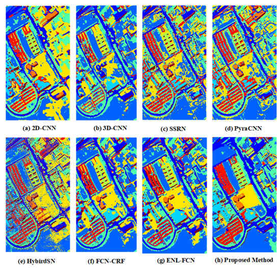
Figure 10. Visualization of the classification maps for the Pavia University dataset.

Table 3. The amount of training, as well as testing, samples for the Pavia University dataset.

No.	Land Cover Class	Training	Testing	Total
1	Asphalt	67	6564	6631
2	Meadows	187	18,462	18,649
3	Gravel	21	2078	2099
4	Trees	31	3033	3064
5	Metal sheets	14	1331	1345
6	Bare Soil	51	4978	5029
7	Bitumen	14	1316	1330
8	Bricks	37	3645	3682
9	Shadows	10	937	947
	Total	432	42,344	42,776

In hyperspectral images, the surface of the same type of target will have chromatic aberrations. Traditional classification methods will make wrong classifications when dealing with such problems, resulting in noises in the classification results. The chromatic aberration on the object’s surface is unclear in some spectral bands. Paying attention to these spectral bands during the classification process will help to correct the classification. Our proposed multi-source fusion attention mechanism incorporates the screening of spectral channels while considering spatial information. From the details, Figure 11 shows that our method has fewer misclassifications compared to ENL-FCN, because our classification process is insensitive to the chromatic aberration of the same types of objects’ surfaces. From the overall view, Figure 10 shows that our method generates less noisy images.

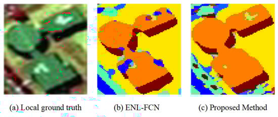
Figure 11. Local classification maps on Pavia University dataset.

To better compare the experiment results, we used four metrics to evaluate the effect of our experiments: the accuracy of each class, the overall accuracies (OA), the average accuracy (AA), and the kappa coefficients. We compared the experimental results of the proposed method with other deep learning algorithms, 2D-CNN [32], 3D-CNN [33], SSRN [34], PyraCNN [53], HybirdSN [54], FCN-CRF [36], and ENL-FCN [30]. The best accuracy is highlighted in bold.

As shown in Table 4, our method also provides the best classification performance in terms of OA, AA, and kappa coefficient for the PU dataset. The PU dataset has $610\times 340$ pixels, so the spatial information is essential for the classification performance. Compared with other methods, the OA of our method is up to $99.3\%$; the AA and the kappa coefficient of our method are up to $99\%$. Although only $1\%$ of the labeled samples are selected for training, our method has achieved the best classification performance.

Table 4. The classification results of 2D-CNN, 3D-CNN, SSRN, PyraCNN, HybirdSN, FCN-CRF, ENL-FCN, and the proposed method on the Pavia University dataset with $1\%$ labeled samples.

Class	2D-CNN	3D-CNN	SSRN	PyraCNN	HybridSN	FCN-CRF	ENL-FCN	Proposed (add)	Proposed (cat)	Proposed (mul)
1	92.72	87.21	99.66	94.94	95.13	91.89	99.40	97.96	97.96	99.30
2	97.14	94.10	98.70	99.41	99.16	95.83	100.00	99.99	99.99	100
3	87.91	64.08	93.95	81.90	88.73	95.82	91.45	99.47	99.47	96.56
4	99.35	96.82	99.72	93.75	98.18	98.23	97.55	96.73	96.73	96.60
5	98.92	95.13	99.93	99.78	98.98	99.67	100.00	100	100	100
6	97.41	94.07	98.52	93.91	98.66	94.76	99.28	100	100	100
7	91.99	58.80	96.84	83.03	96.64	95.42	98.66	99.77	99.77	99.62
8	88.41	77.11	88.85	89.20	90.69	94.95	99.26	99.78	99.78	98.81
9	99.41	84.19	99.53	99.84	97.21	99.77	98.24	99.79	99.79	99.46
OA	95.35	88.69	97.54	95.44	97.01	95.36	99.08	99.38	99.38	99.34
AA	94.81	83.50	97.30	92.86	95.93	96.26	98.20	99.28	99.28	98.93
kappa	93.81	84.86	96.74	93.93	96.02	93.83	98.78	99.18	99.18	99.14

4.4. Experiment 3: Indian Pines Dataset

Indian Pines is a hyperspectral image segmentation dataset. The pixels of the hyperspectral image are $145\times 145$, containing 220 spectral reflectance bands. We used 200 bands, excluding noise bands. There are 10,366 labeled pixels in Indian Pines ground truth, covering 16 land-cover classes. Figure 12 shows the Indian Pines dataset. Figure 13a–h illuminate the classification output using 2D-CNN [32], 3D-CNN [33], SSRN [34], PyraCNN [53], HybirdSN [54], FCN-CRF [36], ENL-FCN [30], and our proposed method. Table 5 lists the number of training and testing data per class. A total of $10\%$ of the data were used as training samples, and the remaining data were tested to assess the model.

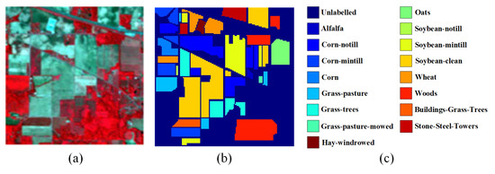
Figure 12. The Indian Pines dataset. (a) Three-band false color composite. (b) Ground-truth map. (c) Legend.

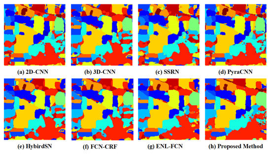
Figure 13. The classification maps for the India Pines dataset were visualized.

Table 5. The amount of training and testing samples for the Indian Pines dataset.

No.	Land Cover Class	Training	Testing	Total
1	Alfalfa	5	49	54
2	Corn-notill	143	1291	1434
3	Corn-mintill	83	751	834
4	Corn	23	211	234
5	Grass-pasture	49	448	497
6	Grass-trees	74	451	525
7	Grass-pasture-mowed	2	24	26
8	Hay-windrowed	48	441	489
9	Oats	2	18	20
10	Soybean-notill	96	872	968
11	Soybean-mintill	246	2222	2468
12	Soybean-clean	61	553	614
13	Wheat	21	191	212
14	Woods	129	1165	1294
15	Buildings-Grass-Trees	38	342	380
16	Stone-Steel-Towers	9	86	95
	Total	1029	9337	10,366

We used four evaluation results indicators, the accuracy of each class, the overall accuracies (OA), the average accuracy (AA), and kappa coefficients, to quantitatively evaluate and compare our method with 2D-CNN [32], 3D-CNN [33], SSRN [34], PyraCNN [53], HybirdSN [54], FCN-CRF [36], and ENL-FCN [30]. From Table 6, we can observe that the proposed method has achieved better classification performances than other methods. The IP dataset contains 145 × 145 pixels, with a lower spatial resolution than KSC and PU datasets. The overall accuracy was $~2\%$ higher than other methods.

Table 6. The classification results of 2D-CNN, 3D-CNN, SSRN, PyraCNN, HybirdSN, FCN-CRF, ENL-FCN, and the proposed method on the Indian Pines dataset with $10\%$ labeled samples.

Class	2D-CNN	3D-CNN	SSRN	PyraCNN	HybridSN	FCN-CRF	ENL-FCN	Proposed (add)	Proposed (cat)	Proposed (mul)
1	100	99.41	98.18	97.26	97.16	96.76	97.15	100	100	100
2	94.11	96.07	96.25	98.99	97.15	95.46	97.86	97.80	99.06	98.19
3	93.69	94.65	96.84	98.96	98.25	94.78	99.75	98.51	99.06	98.51
4	95.40	97.65	97.16	95.54	97.9	90.40	96.60	99.53	99.53	96.21
5	96.87	98.76	99.03	98.79	98.49	94.24	99.26	100	99.30	99.06
6	98.35	98.00	98.61	99.43	98.92	98.42	99.13	99.39	99.69	99.54
7	100	98.82	98.03	89.00	100	83.33	100.00	100	100	100
8	96.58	99.09	99.45	100	99.67	99.56	99.84	100	100	100
9	100	95.00	97.64	91.67	92.38	88.54	85.19	83.33	88.89	83.33
10	94.27	96.18	95.21	95.37	98.74	95.88	98.22	98.95	99.19	99.07
11	95.81	96.08	96.68	98.98	99.16	98.22	99.82	99.77	99.50	99.68
12	93.74	97.02	96.04	95.23	97.47	92.46	99.40	99.43	98.86	99.62
13	99.68	99.78	99.58	100.00	98.02	98.57	98.91	97.81	98.36	97.81
14	98.39	98.82	99.30	98.34	99.32	98.36	99.91	100	100	100
15	95.67	94.72	95.71	94.60	97.64	93.71	93.00	98.26	99.13	98.84
16	94.48	95.48	95.48	96.43	91.02	96.44	93.57	96.39	95.18	96.39
OA	95.79	96.84	97.19	98.12	98.44	96.48	98.85	99.34	99.37	99.36
AA	96.69	97.22	97.45	96.79	97.58	94.80	97.35	98.20	98.65	98.07
kappa	95.10	96.40	96.80	97.85	98.23	95.98	98.69	99.25	99.29	99.27

5. Discussion

To better understand the effectiveness of the multi-source fusion attention mechanism in the framework, we conduct experiments on the proposed attention mechanism. Experiments were performed on the three different datasets with different spatial resolutions and channels.

For discussion on the multi-source fused attention mechanism, Table 7 lists the results of the baseline with the multi-source fusion attention mechanism on the Kennedy Space Center (KSC), Pavia University (PU), and Indian Pines (IP) datasets. The baseline method is one that only employs the swin transformer [45] as the encoder.

Table 7. Effectiveness analysis of the multi-source fused attention mechanism on the three datasets.

KSC
	OA	AA	Kappa
Baseline	99.48	99.27	99.42
Attention add	99.90	99.85	99.89
Attention cat	99.98	99.98	99.98
Attention mul	99.75	99.70	99.73
PU
	OA	AA	Kappa
Baseline	99.32	99.13	99.11
Attention add	99.38	99.28	99.18
Attention cat	99.38	99.28	99.18
Attention mul	99.34	98.93	99.14
IP
	OA	AA	Kappa
Baseline	99.40	98.30	99.34
Attention add	99.34	98.20	99.25
Attention cat	99.37	98.65	99.29
Attention mul	99.36	98.07	99.27

Taking the Kennedy Space Center dataset, for example, the multi-source fusion attention mechanism is added to the framework, and OA, AA, and kappa coefficient increased 0.5 percentage points. The concatenated way achieves the best results among the three means of integrating spatial attention and spectral-channel attention. The classification performance in Pavia University and Indian Pines (IP) datasets is slightly different; the OA, AA, and kappa coefficient have little difference. The reason is that the KSC dataset has a higher spatial resolution and fewer channels. The multi-source fused attention mechanism is evident at high spatial resolution. When the spatial resolution is low, the spatial information is sufficient to achieve a comparable classification effect. Overall, by introducing the multi-source fusion attention with the transformer, the framework can boost the hyperspectral image classification accuracy.

6. Conclusions

In this paper, we proposed an encoder–decoder network to learn the global context information for hyperspectral image (HSI) classification. In the network, a multi-source fusion attention mechanism is proposed to model global semantic information and notice meaningful channels. Based on our multi-source fusion attention mechanism, we proposed a hierarchical encoding transformer structure to extract local and global information. In order to efficiently use the features of different scales obtained by encoding, our decoder fuses the features of the encoder part by means of a suitable upsampling method, skip connections, as well as convolution blocks. Our proposed method can effectively avoid the interference of the same type of object chromatic aberration, thus enabling efficient feature encoding from fewer data. We conducted experiments on three public datasets to validate the excellent performance of the model, including the Kennedy Space Center dataset (OA: 99.98, AA: 99.98, kappa: 99.98), Pavia University dataset (OA: 99.38, AA: 99.28, kappa: 99.18), and Indian Pines dataset (OA: 99.37, AA: 98.65, kappa: 99.29). Compared with other state-of-the-art methods, our approach has greater performance in hyperspectral image classification. However, our method is still inadequate in dealing with the details of hyperspectral images. In future work, we plan to investigate the use of more advanced methods to design attention mechanisms to achieve higher performances for hyperspectral image classifications.

References

- Li, S.; Song, W.; Fang, L.; Chen, Y.; Ghamisi, P.; Atli Benediktsson, J. Deep learning for hyperspectral image classification: An overview. IEEE Trans. Geosci. Remote Sens. 2019, 57, 6690–6709. [Google Scholar] [CrossRef] [Green Version]
- Govender, M.; Chetty, K.; Bulcock, H. A review of hyperspectral remote sensing and its application in vegetation and water resource studies. Water Sa 2007, 33, 145–151. [Google Scholar] [CrossRef] [Green Version]
- Adam, E.; Mutanga, O.; Rugege, D. Multispectral and hyperspectral remote sensing for identification and mapping of wetland vegetation: A review. Wetl. Ecol. Manag. 2010, 18, 281–296. [Google Scholar] [CrossRef]
- Koch, B. Status and future of laser scanning, synthetic aperture radar and hyperspectral remote sensing data for forest biomass assessment. ISPRS J. Photogramm. Remote Sens. 2010, 65, 581–590. [Google Scholar] [CrossRef]
- Camps-Valls, G.; Tuia, D.; Bruzzone, L.; Benediktsson, J.A. Advances in hyperspectral image classification: Earth monitoring with statistical learning methods. IEEE Signal Process. Mag. 2013, 31, 45–54. [Google Scholar] [CrossRef] [Green Version]
- Gislason, P.O.; Benediktsson, J.A.; Sveinsson, J.R. Random forests for land cover classification. Pattern Recognit. Lett. 2006, 27, 294–300. [Google Scholar] [CrossRef]
- Melgani, F.; Bruzzone, L. Classification of hyperspectral remote sensing images with support vector machines. IEEE Trans. Geosci. Remote Sens. 2004, 42, 1778–1790. [Google Scholar] [CrossRef] [Green Version]
- Rainforth, T.; Wood, F. Canonical correlation forests. arXiv 2015, arXiv:1507.05444. [Google Scholar]
- Xia, J.; Yokoya, N.; Iwasaki, A. Hyperspectral image classification with canonical correlation forests. IEEE Trans. Geosci. Remote Sens. 2016, 55, 421–431. [Google Scholar] [CrossRef]
- Krishnapuram, B.; Carin, L.; Figueiredo, M.A.T.; J Hartemink, A. Sparse multinomial logistic regression: Fast algorithms and generalization bounds. IEEE Trans. Pattern Anal. Mach. Intell. 2005, 27, 957–968. [Google Scholar] [CrossRef] [Green Version]
- Xia, J.; Du, P.; He, X.; Chanussot, J. Hyperspectral remote sensing image classification based on rotation forest. IEEE Geosci. Remote Sens. Lett. 2013, 11, 239–243. [Google Scholar] [CrossRef] [Green Version]
- Fauvel, M.; Benediktsson, J.A.; Chanussot, J.; R Sveinsson, J. Spectral and spatial classification of hyperspectral data using svms and morphological profiles. IEEE Trans. Geosci. Remote Sens. 2008, 46, 3804–3814. [Google Scholar] [CrossRef] [Green Version]
- Tarabalka, Y.; Benediktsson, J.A.; Chanussot, J. Spectral–spatial classification of hyperspectral imagery based on partitional clustering techniques. IEEE Trans. Geosci. Remote Sens. 2009, 47, 2973–2987. [Google Scholar] [CrossRef]
- Li, J.; Bioucas-Dias, J.M.; Plaza, A. Spectral–spatial classification of hyperspectral data using loopy belief propagation and active learning. IEEE Trans. Geosci. Remote Sens. 2012, 51, 844–856. [Google Scholar] [CrossRef]
- Yue, J.; Zhao, W.; Mao, S.; Liu, H. Spectral—spatial classification of hyperspectral images using deep convolutional neural networks. Remote Sens. Lett. 2015, 6, 468–477. [Google Scholar] [CrossRef]
- Hu, W.; Huang, Y.; Wei, L.; Zhang, F.; Li, H. Deep convolutional neural networks for hyperspectral image classification. J. Sens. 2015, 2015, 258619. [Google Scholar] [CrossRef] [Green Version]
- Chen, Y.; Jiang, H.; Li, C.; Jia, X.; Ghamisi, P. Deep feature extraction and classification of hyperspectral images based on convolutional neural networks. IEEE Trans. Geosci. Remote Sens. 2016, 54, 6232–6251. [Google Scholar] [CrossRef] [Green Version]
- Yu, S.; Jia, S.; Xu, C. Convolutional neural networks for hyperspectral image classification. Neurocomputing 2017, 219, 88–98. [Google Scholar] [CrossRef]
- Audebert, N.; Saux, B.L.; Lefèvre, S. Deep learning for classification of hyperspectral data: A comparative review. IEEE Geosci. Remote Sens. Mag. 2019, 7, 159–173. [Google Scholar] [CrossRef] [Green Version]
- Xu, Q.; Xiao, Y.; Wang, D.; Luo, B. Csa-mso3dcnn: Multiscale octave 3d cnn with channel and spatial attention for hyperspectral image classification. Remote Sens. 2020, 12, 188. [Google Scholar] [CrossRef] [Green Version]
- Mou, L.; Ghamisi, P.; Zhu, X.X. Deep recurrent neural networks for hyperspectral image classification. IEEE Trans. Geosci. Remote Sens. 2017, 55, 3639–3655. [Google Scholar] [CrossRef] [Green Version]
- Hang, R.; Liu, Q.; Hong, D.; Ghamisi, P. Cascaded recurrent neural networks for hyperspectral image classification. IEEE Trans. Geosci. Remote Sens. 2019, 57, 5384–5394. [Google Scholar] [CrossRef] [Green Version]
- Hamida, A.B.; Benoit, A.; Lambert, P.; Amar, C.B. 3-d deep learning approach for remote sensing image classification. IEEE Trans. Geosci. Remote Sens. 2018, 56, 4420–4434. [Google Scholar] [CrossRef] [Green Version]
- Wu, H.; Prasad, S. Convolutional recurrent neural networks forhyperspectral data classification. Remote Sens. 2017, 9, 298. [Google Scholar] [CrossRef] [Green Version]
- Lee, H.; Kwon, H. Going deeper with contextual cnn for hyperspectral image classification. IEEE Trans. Image Process. 2017, 26, 4843–4855. [Google Scholar] [CrossRef] [PubMed] [Green Version]
- He, X.; Chen, Y.; Ghamisi, P. Heterogeneous transfer learning for hyperspectral image classification based on convolutional neural network. IEEE Trans. Geosci. Remote Sens. 2019, 58, 3246–3263. [Google Scholar] [CrossRef]
- Gong, Z.; Zhong, P.; Yu, Y.; Hu, W.; Li, S. A cnn with multiscale convolution and diversified metric for hyperspectral image classification. IEEE Trans. Geosci. Remote Sens. 2019, 57, 3599–3618. [Google Scholar] [CrossRef]
- Paoletti, M.E.; Haut, J.M.; Plaza, J.; Plaza, A. Deep learning classifiers for hyperspectral imaging: A review. ISPRS J. Photogramm. Remote Sens. 2019, 158, 279–317. [Google Scholar] [CrossRef]
- Feng, Z.; Yang, S.; Wang, M.; Jiao, L. Learning dual geometric low-rank structure for semisupervised hyperspectral image classification. IEEE Trans. Cybern. 2019, 51, 346–358. [Google Scholar] [CrossRef]
- Shen, Y.; Zhu, S.; Chen, C.; Du, Q.; Xiao, L.; Chen, J.; Pan, D. Efficient deep learning of nonlocal features for hyperspectral image classification. IEEE Trans. Geosci. Remote Sens. 2020, 59, 6029–6043. [Google Scholar] [CrossRef]
- Ruck, D.W.; Rogers, S.K.; Kabrisky, M. Feature selection using a multilayer perceptron. J. Neural Netw. Comput. 1990, 2, 40–48. [Google Scholar]
- Makantasis, K.; Karantzalos, K.; Doulamis, A.; Doulamis, N. Deep supervised learning for hyperspectral data classification through convolutional neural networks. In Proceedings of the 2015 IEEE International Geoscience and Remote Sensing Symposium (IGARSS), Milan, Italy, 26–31 July 2015; pp. 4959–4962. [Google Scholar]
- Li, Y.; Zhang, H.; Shen, Q. Spectral–spatial classification of hyperspectral imagery with 3d convolutional neural network. Remote Sens. 2017, 9, 67. [Google Scholar] [CrossRef] [Green Version]
- Zhong, Z.; Li, J.; Luo, Z.; Chapman, M. Spectral–spatial residual network for hyperspectral image classification: A 3-d deep learning framework. IEEE Trans. Geosci. Remote Sens. 2017, 56, 847–858. [Google Scholar] [CrossRef]
- Ma, W.; Yang, Q.; Wu, Y.; Zhao, W.; Zhang, X. Double-branch multi-attention mechanism network for hyperspectral image classification. Remote Sens. 2019, 11, 1307. [Google Scholar] [CrossRef] [Green Version]
- Xu, Y.; Du, B.; Zhang, L. Beyond the patchwise classification: Spectral-spatial fully convolutional networks for hyperspectral image classification. IEEE Trans. Big Data 2019, 6, 492–506. [Google Scholar] [CrossRef]
- Xu, Y.; Zhang, L.; Du, B.; Zhang, F. Spectral–spatial unified networks for hyperspectral image classification. IEEE Trans. Geosci. Remote Sens. 2018, 56, 5893–5909. [Google Scholar] [CrossRef]
- Ronneberger, O.; Fischer, P.; Brox, T. U-net: Convolutional networks for biomedical image segmentation. In International Conference on Medical Image Computing and Computer-Assisted Intervention; Springer: Berlin, Germany, 2015; pp. 234–241. [Google Scholar]
- Zheng, Z.; Zhong, Y.; Ma, A.; Zhang, L. Fpga: Fast patch-free global learning framework for fully end-to-end hyperspectral image classification. IEEE Trans. Geosci. Remote Sens. 2020, 58, 5612–5626. [Google Scholar] [CrossRef]
- Zhu, Q.; Deng, W.; Zheng, Z.; Zhong, Y.; Guan, Q.; Lin, W.; Zhang, L.; Li, D. A spectral-spatial-dependent global learning framework for insufficient and imbalanced hyperspectral image classification. IEEE Trans. Cybern. 2021. [Google Scholar] [CrossRef]
- Vaswani, A.; Shazeer, N.; Parmar, N.; Uszkoreit, J.; Jones, L.; Gomez, A.N.; Kaiser, Ł.; Polosukhin, I. Attention is all you need. Adv. Neural Inf. Process. Syst. 2017, 30, 675–686. [Google Scholar]
- Tian, L.; Tu, Z.; Zhang, D.; Liu, J.; Li, B.; Yuan, J. Unsupervised learning of optical flow with cnn-based non-local filtering. IEEE Trans. Image Process. 2020, 29, 8429–8442. [Google Scholar] [CrossRef]
- Dosovitskiy, A.; Beyer, L.; Kolesnikov, A.; Weissenborn, D.; Zhai, X.; Unterthiner, T.; Dehghani, M.; Minderer, M.; Heigold, G.; Gelly, S.; et al. An image is worth 16 × 16 words: Transformers for image recognition at scale. arXiv 2020, arXiv:2010.11929. [Google Scholar]
- Touvron, H.; Cord, M.; Douze, M.; Massa, F.; Sablayrolles, A.; Jégou, H. Training data-efficient image transformers & distillation through attention. In Proceedings of the International Conference on Machine Learning, Virtual Event, 18–24 July 2021; pp. 10347–10357. [Google Scholar]
- Liu, Z.; Lin, Y.; Cao, Y.; Hu, H.; Wei, Y.; Zhang, Z.; Lin, S.; Guo, B. swin transformer: Hierarchical vision transformer using shifted windows. In Proceedings of the IEEE/CVF International Conference on Computer Vision, Virtual Event, 12 October 2021; pp. 10012–10022. [Google Scholar]
- Han, K.; Xiao, A.; Wu, E.; Guo, J.; Xu, C.; Wang, Y. Transformer in transformer. Adv. Neural Inf. Process. Syst. 2021, 34, 1056–1067. [Google Scholar]
- Wang, W.; Xie, E.; Li, X.; Fan, D.-P.; Song, K.; Liang, D.-P.; Lu, T.; Luo, P.; Shao, L. Pyramid vision transformer: A versatile backbone for dense prediction without convolutions. In Proceedings of the IEEE/CVF International Conference on Computer Vision, Virtual Event, 12 October 2021; pp. 568–578. [Google Scholar]
- Bao, H.; Dong, L.; Wei, F.; Wang, W.; Yang, N.; Liu, X.; Wang, Y.; Gao, J.; Piao, S.; Zhou, M.; et al. Unilmv2: Pseudo-masked language models for unified language model pre-training. In Proceedings of the International Conference on Machine Learning, Vienna, Austria, 13–18 July 2020; PMLR: Stockholm, Sweden, 2020; pp. 642–652. [Google Scholar]
- Hu, H.; Gu, J.; Zhang, Z.; Dai, J.; Wei, Y. Relation networks for object detection. In Proceedings of the IEEE Conference on Computer Vision and Pattern Recognition, Salt Lake City, UT, USA, 18–23 June 2018; pp. 3588–3597. [Google Scholar]
- Hu, H.; Zhang, Z.; Xie, Z.; Lin, S. Local relation networks for image recognition. In Proceedings of the IEEE/CVF International Conference on Computer Vision, Seoul, Korea, 27 October–2 November 2019; pp. 3464–3473. [Google Scholar]
- Gardner, M.W.; Dorling, S.R. Artificial neural networks (the multilayer perceptron)—A review of applications in the atmospheric sciences. Atmos. Environ. 1998, 32, 2627–2636. [Google Scholar] [CrossRef]
- Kim, S.W.; Kook, H.K.; Sun, J.Y.; Kang, M.C.; Ko, S.J. Parallel feature pyramid network for object detection. In Proceedings of the European Conference on Computer Vision (ECCV), Munich, Germany, 8–14 September 2018; pp. 234–250. [Google Scholar]
- Paoletti, M.E.; Haut, J.M.; Fernandez-Beltran, R.; Plaza, J.; Plaza, A.J.; Pla, F. Deep pyramidal residual networks for spectral–spatial hyperspectral image classification. IEEE Trans. Geosci. Remote Sens. 2018, 57, 740–754. [Google Scholar] [CrossRef]
- Roy, S.K.; Krishna, G.; Dubey, S.R.; Chaudhuri, B.B. Hybridsn: Exploring 3-d–2-d cnn feature hierarchy for hyperspectral image classification. IEEE Geosci. Remote Sens. Lett. 2019, 17, 277–281. [Google Scholar] [CrossRef] [Green Version]
Publisher’s Note: MDPI stays neutral with regard to jurisdictional claims in published maps and institutional affiliations. |
© 2022 by the authors. Licensee MDPI, Basel, Switzerland. This article is an open access article distributed under the terms and conditions of the Creative Commons Attribution (CC BY) license (https://creativecommons.org/licenses/by/4.0/).