Abstract
Accurate combined bundle adjustment (BA) is a fundamental step for the integration of aerial and terrestrial images captured from complementary platforms. In traditional photogrammetry pipelines, self-calibrated bundle adjustment (SCBA) improves the BA accuracy by simultaneously refining the interior orientation parameters (IOPs), including lens distortion parameters, and the exterior orientation parameters (EOPs). Aerial and terrestrial images separately processed through SCBA need to be fused using BA. Thus, the IOPs in the aerial–terrestrial BA must be properly treated. On one hand, the IOPs in one flight should be identical for the same images in physics. On the other hand, the IOP adjustment in the cross-platform-combined BA may mathematically improve the aerial–terrestrial image co-registration degree in 3D space. In this paper, the impacts of self-calibration strategies in combined BA of aerial and terrestrial image blocks on the co-registration accuracy were investigated. To answer this question, aerial and terrestrial images captured from seven study areas were tested under four aerial–terrestrial BA scenarios: the IOPs for both aerial and terrestrial images were fixed; the IOPs for only aerial images were fixed; the IOPs for only terrestrial images were fixed; the IOPs for both images were adjusted. The cross-platform co-registration accuracy for the BA was evaluated according to independent checkpoints that were visible on the two platforms. The experimental results revealed that the recovered IOPs of aerial images should be fixed during the BA. However, when the tie points of the terrestrial images are comprehensively distributed in the image space and the aerial image networks are sufficiently stable, refining the IOPs of the terrestrial cameras during the BA may improve the co-registration accuracy. Otherwise, fixing the IOPs is the best solution.
1. Introduction
Multi-view images captured by aerial or unmanned aerial vehicle (UAV) platforms have become a major source of data in 3D city modeling projects [1,2,3,4]. To alleviate occlusions and increase observation redundancy, in the last decade, images captured by different cameras, such as vertical and oblique views in multi-camera systems, are combined to product photo-realistic 3D models with better geometry quality and textures [5,6,7].
Because the accuracy of modeling image distortions and orientations directly affects the product quality in subsequent image-processing steps such as dense image matching, 3D mesh generation, and texture mapping, numerous methods have been developed to recover EOPs and IOPs (including lens distortion parameters) [8,9,10,11,12].
Among existing photogrammetry research and engineering practices, self-calibrated bundle adjustment (SCBA), through which IOPs and EOPs are simultaneously estimated according to image tie points, is an effective method for decreasing re-projection errors in 2D space and intersection errors in 3D space [13,14,15,16,17]. Different from the traditional laboratory or field calibration processes, self-calibration (SC) methods treat IOP calibration as part of routine photogrammetric procedures in every project through bundle adjustment (BA), whether the cameras have been pre-calibrated or not [18].
In recent years, terrestrial images captured by hand-held cameras or mobile mapping platforms have been integrated with aerial views through structure-from-motion and multi-view stereo pipelines to produce better 3D maps and models [19,20,21,22]. Due to large differences in viewpoint and scale and possible illumination conditions, automatic feature matching for cross-platform images is non-trivial work [21]. The numbers and distributions of cross-platform tie points are not as favorable as those for inner-platform images. Hence, in 3D modeling applications that integrate images captured by aerial and terrestrial platforms, images taken in the same platform are often first aligned through BA using only inner-platform tie points. Then, aerial and terrestrial images are co-registered using a cross-platform involving BA [19,20,21]. Although IOPs should be refined during the inner-platform BA, it remains unclear whether the IOPs in the cross-platform BA should be fixed.
On one hand, the IOPs are recovered through SCBA with inner-platform tie points, and the images used in the cross-platform remain unchanged; thus, the IOPs in the second BA should be physically the same as those in the first BA. IOP fixation could reduce the number of unknown parameters and stabilize the calculation of the nonlinear least square problem. On the other hand, according to SCBA theory, refining the IOPs in the cross-platform BA may mathematically improve the modeling quality of the image formatting process and thus enhance the co-registration quality between the aerial and terrestrial images.
Both strategies seem reasonable. Hence, to investigate the optimal SC strategy for the BA of aerial–terrestrial integrated images, four aerial–terrestrial BA settings were experimentally compared and analyzed in this study. According to the experimental results, recommendations on the integration of aerial and terrestrial images blocks in BA are provided.
The remainder of this paper is organized as follows: Section 2 reviews the existing work on SCBA. Section 3 introduces the four plausible SCBA strategies and the experimental datasets and procedure. Section 4 reports the experimental results and analysis. Section 5 presents the discussion, conclusions, and future perspectives.
2. Related Works
The geometry quality of image-based 3D mapping products largely relies on the precision of the recovered image IOPs and EOPs [23]. In traditional photogrammetry engineering, the IOPs of metric cameras are first calibrated in the laboratory or field before image capture [9,13,24]. After image collection, EOPs are recovered through BA according to image correspondence and a few ground control points [4,25,26]. Previous investigations have proved that when a sufficiently accurate camera model is used, the 3D mapping inaccuracy related to systematic errors in IOPs is negligible [27]; however, this is not the case in close-range photogrammetry [28,29].
With the rapid development of UAVs, consumer-level cameras are widely used in small- or clustered-area survey tasks [30,31,32,33,34,35]. Compared with traditional aerial photogrammetry, which collects images with only vertical views, adding oblique cameras could not only result in better façade information but also favor geometry measuring accuracy due to the larger intersection angles between overlapped images [6,36,37]. This advantage is more noticeable for UAV photogrammetry since the flight plans are far more flexible [38,39]. While image collection is relatively easy, a rigorous laboratory or field camera calibration process is often neglected. Moreover, the images are often captured by unprofessional operators with inferior geometry networks. Furthermore, the sensor stability may be imperfect, as 3D mapping and modeling are not the main purposes of the camera design.
Hence, in most UAV photogrammetry applications, SCBA is commonly adopted to refine the IOPs to improve the 3D accuracy of object mapping [3,26,32,40]. In standard SCBA, the IOPs are treated as unknown parameters with initial observations; moreover, the IOPs, EOPs, and 3D coordinates of tie points during the BA process are refined according to the collinearity equation [18]. Regarding the sensor stability under different temperatures and humidities, SCBA is often conducted in every image block, because the images are collected under various conditions.
Apart from the conventional focal length and the location of principal points, additional parameters are used to describe the distortions that occur between 3D points and their locations in 2D images, because the image formatting process is not a perfect perspective transformation [24]. As pointed out in previous works [41], there are two major categories of additional parameters: the physical and mathematical models [13,41,42]. The physical models simulate the systematic errors caused by optics, while the mathematical models approximate the simulation process through algebra expansion.
The Brown model [13] is the most widely used model in close-range photogrammetry, and it has been incorporated into numerous image-processing packages and commercial softwares in United States, China, and Russia [43,44,45]. Although SCBA implementation with additional parameters may improve geometric accuracy in practice, the correlation between parameters may weaken the BA process [18]. Moreover, to obtain satisfactory results, a large number and good distribution of image tie points are required [46].
In recent years, 3D environmental modeling applications have combined images captured by airborne cameras and terrestrial platforms [20,21,39]. Images captured by a singular platform and processed through BA also require cross-platform BA for accurate co-registration in 3D mapping and modeling tasks [19].
In addition to the viewing perspective and image scales, images obtained by aerial and terrestrial platforms also vary in other aspects. First, the networks for aerial images are often more stable, because aerial views have more image connectivity than terrestrial views. Moreover, owing to the differences in looking directions and scenes, terrestrial images might have weak textures at the corners or edges. Thus, the distributions of automatic tie points are often more unsymmetrical than for aerial datasets.
However, it is still unclear whether it is best to re-compute the IOPs during the BA of aerial and terrestrial images. On one hand, the SCBA are already adopted in the BA, which align images captured by the same platform; the IOPs can be treated as stable because the images remain unchanged [19]. Moreover, IOP fixation can reduce the number of unknown parameters, which may stabilize the EOP calculation process and possibly enhance the estimation accuracy. Furthermore, the additional cross-platform tie points that align aerial and terrestrial images can result in uneven tie point distribution [39]. Because more tie points (mainly the cross-platform tie points) are incorporated into the BA process, the image geometric network is varied. From a mathematical viewpoint, the integrated refinement of both IOPs and EOPs may improve the recovery of the image formatting process and thereby improve the co-registration between aerial and terrestrial images.
To investigate the optimal SC strategy for the BA of aerial–terrestrial integrated images after the inner-platform SCBA, four SC strategies for the BA were compared and analyzed using real datasets.
3. Experimental Settings and Datasets
3.1. Experimental Hypothesis and Settings
To evaluate the performances of different SCBA strategies for aerial–terrestrial image blocks (Figure 1), the following procedures were adopted. Starting from aerial and terrestrial images with initial EOPs and IOPs in seven study sites, a SCBA was separately adopted for aerial and terrestrial images, and the updated EOPs and IOPs were obtained. Then, BA was implemented to integrate aerial and terrestrial images. In the BA, four SC strategies were used: (1) fixing the IOPs for both aerial and terrestrial images (FA_FT); (2) fixing the IOPs for aerial images while refining the IOPs for terrestrial images (FA_RT); (3) refining the IOPs for aerial images while fixing the IOPs for terrestrial images (RA_FT); (4) refining the IOPs for both aerial and terrestrial images (RA_RT). After the implementation of BA, IOPs and EOPs for aerial and terrestrial images were obtained.
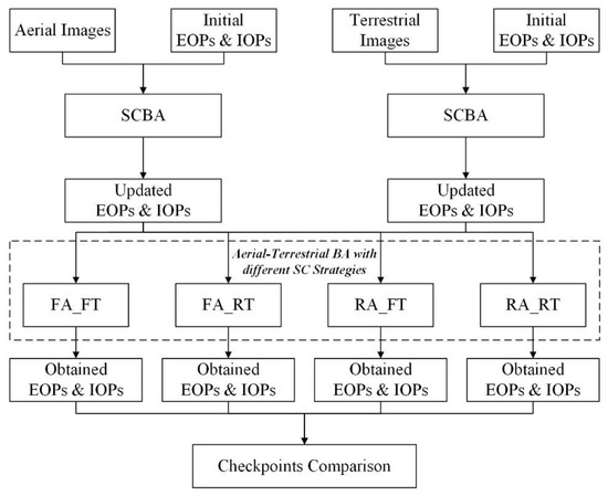
Figure 1.
The overall workflow of the study.
In this study, the camera was the classic pinhole model; the lens distortion parameter is given in Equation (1).
where X, a 3D column vector, represents the 3D position of a point in the object space, and x, a 2D vector, denotes the position of the corresponding point in the image space. Xc and R are the EOPs, where Xc is the 3D position of the camera center, while R represents a 3 × 3 rotation matrix that maps between the axes of world coordinates and the camera axes. f denotes the focal length, and x0 denotes the position of the principal point. represents the perspective projection defined by Equation (2), and u, v, and w represent the coordinates of a 3D point in the camera space. The additional parameters of the lens distortion are given by , where
Here, k1, k2, and k3 denote the radial distortion coefficients, and p1 and p2 represent the tangential distortion coefficients.
To reveal the co-registration accuracy between the aerial and terrestrial datasets, some checkpoints visible in the images captured by the two platforms were selected, measured, and triangulated. For precision, each checkpoint is measured in four images from the same platform at least. Finally, the 3D residuals between the triangulated position of the same checkpoint from the two platforms were computed, and the statistical parameters of mean value, maximum value, variance, and root mean square error (RMSE) were calculated.
3.2. Aerial–Terrestrial Datasets Used in the Experiments
To explore the performance of the different SCBA strategies, seven datasets were used in the experiments, including the benchmark datasets released by the International Society for Photogrammetry and Remote Sensing [47], SWJTU [21], and collected images. Table 1 and Table 2 present some general information on the used image datasets.

Table 1.
Basic information of the test datasets used in the study (GSD: ground sample distance).
Table 2.
Basic information of the cameras used in the study.
The Rathaus, Stadthaus, Pferdestall, Verwaltung, and Lohnhalle datasets were collected from Dortmund, Germany; the SWJTU-LIB dataset was collected from Chengdu, China; the SZU-YPS dataset was captured from Shenzhen, China. In all the tested datasets, most of the aerial (UAV) images are oblique, which would not only broaden the overlapping areas with the terrestrial views but also increase the intersection angles and result in better geometry accuracy for the image blocks. Sample images of the test datasets are shown in Figure 2. As shown in each row of Figure 2, although obvious perspective distortions and scale variations exist between aerial and terrestrial views, the lighting condition between them are rather similar. Therefore, the cross-platform image feature matching is more reliable than on those images with distinct radiometric discrepancies, which creates a good foundation for our cross-platform BA tests.
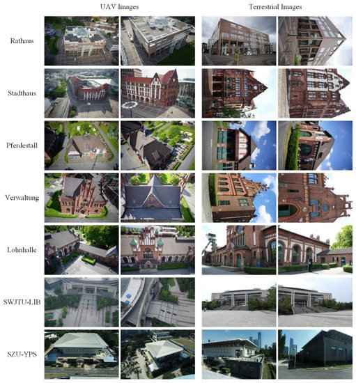
Figure 2.
Sample images of the tested datasets.
The UAV images in the SWJTU-LIB dataset were collected during regular strip flights, while the other aerial (UAV) and terrestrial images were captured surrounding and focusing on target buildings. In all datasets, the GPS information stored in the flights provided absolute ground control, and no ground control points are incorporated in the image orientation process. The SIFT algorithm [48] is implemented to find corresponding points between overlapping images, and the Gauss–Newton method [8] is adopted to solve the nonlinear least square problem in BA.
4. Experimental Results and Analysis
4.1. Experimental Results
The EOPs and sparse point clouds after the BA of both aerial and terrestrial images are shown in Figure 3. In the seven tested areas, aerial and terrestrial images were correctly aligned, which enabled integrated 3D mapping and 3D scene reconstruction. Except for the Stadthaus dataset, the aerial images were captured through convergent shooting strategies, which resulted in stable image networks. Moreover, the terrestrial image networks in the Rathaus and Verwaltung datasets were more stable than those in the other five datasets.
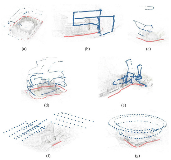
Figure 3.
EOPs of images and sparse point clouds after aerial–terrestrial BA in the tested datasets. The blue and pink squares represent aerial and terrestrial images, respectively. (a) Rathaus; (b) Stadthaus; (c) Pferdestall; (d) Verwaltung; (e) Lohnhalle; (f) SWJTU-LIB; (g) SZU-YPS.
The refined IOPs of the aerial (UAV) and terrestrial images after SCBA, and the IOPs after aerial–terrestrial BA using the four different strategies, are presented in Table 3, Table 4, Table 5, Table 6, Table 7, Table 8 and Table 9. For convenience, the focal lengths and coordinates of the principal points are represented in pixels. As presented in Table 3, Table 4, Table 5, Table 6, Table 7, Table 8 and Table 9, during the refining of the IOPs of aerial images in the BA, the focal lengths after optimization were highly stable, and the differences in focal length between RA_RT, RA_FT, and FA_FT&FA_RT were within 1 pixel. Meanwhile, the corresponding differences for terrestrial images were slightly greater; for example, the focal length after FA_RT BA strategies was greater than the original value of 1 pixel (Table 5). The principal points xp and yp also exhibited the same trend. The differences in xp and yp between the four compared BA strategies were less than 2 pixels in all of the tested datasets for aerial images, but greater than 2 pixels in the tested datasets for terrestrial images. For the Pferdestall dataset, the variations between xp obtained through the FA_RT and FA_FT&RA_FT methods were greater than 3 pixels. For the other additional parameters related to radial distortion and tangential distortion, the adjusted values obtained through the four compared BA strategies were similar.
Table 3.
IOPs of aerial (UAV) and terrestrial images after the BA of the Rathaus dataset using different SC strategies.
Table 4.
IOPs of aerial (UAV) images and terrestrial images after the BA of the Stadthaus dataset using different SC strategies.
Table 5.
IOPs of aerial (UAV) and terrestrial images after the BA of the Pferdestall dataset using different SC strategies.
Table 6.
IOPs of aerial (UAV) and terrestrial images after the BA of the Verwaltung dataset using different SC strategies.
Table 7.
IOPs of aerial (UAV) and terrestrial images after the BA of the Lohnhalle dataset using different SC strategies.
Table 8.
IOPs of aerial (UAV) and terrestrial images after the BA of the SWJTU-LIB dataset using different SC strategies.
Table 9.
IOPs of aerial (UAV) and terrestrial images after the BA of the SZU-YPS dataset using different SC strategies.
The adjusted values of RA_FT and RA_RT for the aerial images were closer to each other than they were to the original values that were only adjusted in the previous SCBA. Consequently, the optimized IOPs of FA_RT and RA_RT for the terrestrial images were closer to each other than they were to the optimized IOPs of FA_FT&RA_FT. As given in Table 1, the UAV images and terrestrial images in Rathaus and Pferdestall were obtained using the same cameras. However, the obtained IOPs were closer to one another in the Rathaus dataset than in the Pferdestall dataset (Table 3 and Table 5).
To verify the performance of co-registration between aerial and terrestrial images processed using the four compared BA strategies, the triangulated 3D positions of some checkpoints that were visible in both the aerial and terrestrial images were compared. Figure 4 illustrates some samples of checkpoints measured in the tested datasets. These points are measured on targets which are intentionally put by the data collectors, and the other CPs are measured on distinct corners in the scenes. For each checkpoint, at least four observations were measured in images captured by one platform, and the maximum back projection errors for checkpoints are limited to one pixel. Eleven to seventeen checkpoints were extracted in each of the seven tested datasets. Most of the checkpoints are distributed on vertical walls because those are the major common visible areas for aerial and terrestrial views. To reach even distribution as fair as possible in both planar and vertical directions, there are also some checkpoints measured on the roof corners and the ground. However, the absolute 3D position for checkpoints has not been measured by any topographic support since this study focuses on the relative cross-platform co-registration accuracy.
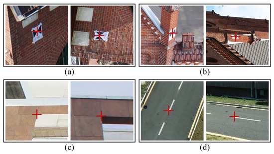
Figure 4.
Samples of checkpoints measured in the tested datasets. In each subgraph, the left is measured in aerial (UAV) image while the right is measured in terrestrial image. (a,b), checkpoints measured on targets; (c,d), checkpoints measured on distinct corners.
The statistics of 3D errors at checkpoints are listed in Table 10. For the seven tested areas, the RMSEs in the X, Y, and Z directions ranged from 4.448 to 202.729 mm. The minimax RMSE values occurred in the Verwaltung dataset, and the maximum values occurred in the SWJTU_LIB dataset. This was possibly due to the occurrence of different image GSDs and image numbers (Table 1). Comparison of the results of different BA strategies revealed that the FA_FT and FA_RT methods exhibited the minimum RMSE values. In Rathaus, Stadthaus, Pferdestall, SWJTU-LIB, and SZU-YPS, the FA_FT method obtained the minimum 3D RMSE values and the minimax deviation values, which corresponded to the highest co-registration accuracies between aerial and terrestrial images.
Table 10.
Statistics of checkpoints. No. CPs: number of checkpoints. RMSE: root mean square error. The values in bold indicate the minimal values in the compared four methods.
To qualitatively reveal the relative co-registration accuracies of the different BA strategies, the relative RMSE (rRMSE) was calculated using Equation (4).
In Equation (4), RMSEi denotes the calculated absolute RMSE value of the current method; n denotes the total number of compared methods. The lower the rRMSE value, the higher the relative co-registration accuracy. Moreover, the mean rRMSE value remained 100 in one test area. The calculated rRMSEs of the seven tested areas calculated using this equation are shown in Figure 5. For the seven tested areas, the rRMSEs obtained using the FA_FT method were less than the mean values. For the Stadthaus and SZU-YPS datasets, the rRMSEs obtained using the FA_FT method were remarkably greater than those obtained using the other three methods. For all datasets except SWJTU-LIB, the rRMSEs obtained using the FA_RT and RA_RT methods were similar. The lowest rRMSEs obtained through FA_RT belonged to the Verwaltung and Lohnhalle datasets, and the RA_RT method obtained unstable results for the SWJTU-LIB dataset. The RA_FT method obtained the largest rRMSEs for four test areas, namely Rathaus, Stadthaus, Verwaltung, and Lohnhalle. For the Lohnhalle dataset, the rRMSE values of the four methods were the closest.
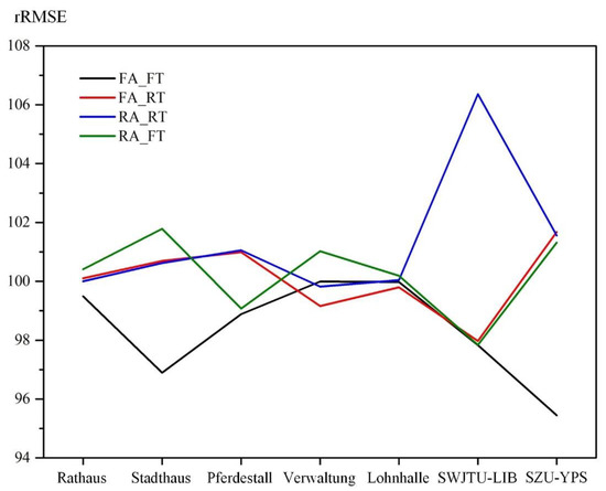
Figure 5.
The rRMSEs of the four compared BA strategies used for the seven tested areas. Different colors indicate different BA methods; black: FA_FT; red: FA_RT; blue: RA_RT; green: RA_FT.
4.2. Experimental Analysis
To further investigate the BA results of aerial and terrestrial images for different SC strategies, the tie point distribution in the image space was plotted and analyzed. Because an even tie point distribution is favorable to the SC process, the uniformities of both aerial and terrestrial tie points were qualitatively and quantitatively evaluated. The image space was equally divided into 100 parts in both the horizontal and vertical directions, and 10,000 grids were created. The number of tie points that belonged to each grid was obtained from the image coordinates of tie points.
These numbers were plotted using heatmaps to visually reveal the tie point distribution for aerial and terrestrial images. The mean values, standard deviations, and normalized standard deviations of the numbers are presented in Table 11. To compare the distribution between different image platforms and datasets, the normalized number of tie points (norNTP) was calculated using Equation (5).
where NTPi denotes the number of tie points in a certain grid, and norNTPi is the normalized value. Thus, the mean value of the normalized number of tie points in each grid was 1. The tie point distributions are illustrated in Figure 6, Figure 7, Figure 8, Figure 9, Figure 10, Figure 11 and Figure 12 using heatmaps generated from the norNTP values and histograms.
Table 11.
Mean values (MVs), standard deviations (STDs), and normalized standard deviations (NSTDs) of the number of points in equant grids.
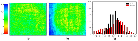
Figure 6.
Tie point distributions for the Rathaus dataset: (a) aerial (UAV) and (b) terrestrial image spaces; (c) histograms.
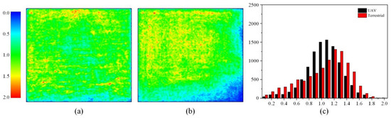
Figure 7.
Tie point distributions for the Stadthaus dataset: (a) aerial (UAV) and (b) terrestrial image spaces; (c) histograms.
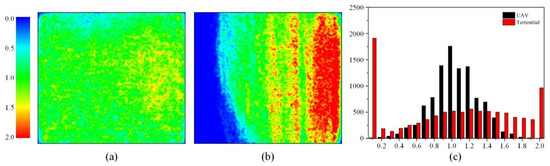
Figure 8.
Tie point distributions for the Pferdestall dataset: (a) aerial (UAV) and (b) terrestrial image spaces; (c) histograms.
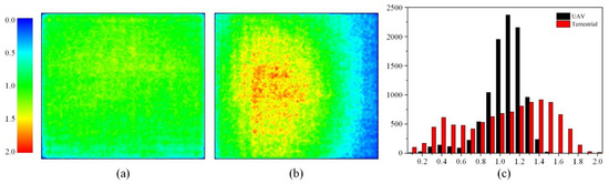
Figure 9.
Tie point distributions for the Verwaltung dataset; (a) aerial (UAV) and (b) terrestrial image spaces; (c) histograms.
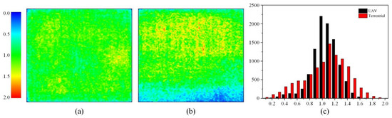
Figure 10.
Tie point distributions for the Lohnhalle dataset: (a) aerial (UAV) and (b) terrestrial image spaces; (c) histograms.
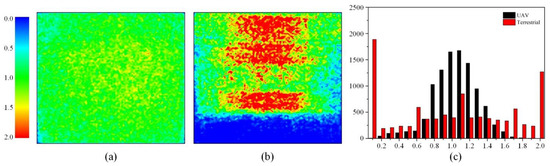
Figure 11.
Tie point distributions for the SWJIT-LIB dataset: (a) aerial (UAV) and (b) terrestrial image spaces; (c) histograms.
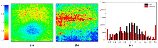
Figure 12.
Tie point distributions for the SZU-YPS dataset: (a) aerial (UAV) and (b) terrestrial image spaces; (c) histograms.
The mean values, standard deviations, and NSTDs of the number of points in equant grids for the tested datasets are given in Table 11. Comparison of the NSTDs between different platforms revealed that in the seven tested datasets, the NSTDs for the aerial images were considerably smaller than those for terrestrial images, indicating that the tie point distribution in the aerial platforms was more uniform than that in the terrestrial platforms.
The NSTD values are consistent with the visual expression of the results in Figure 6, Figure 7, Figure 8, Figure 9, Figure 10,Figure 11 and Figure 12. As illustrated in Figure 6a, Figure 7a, Figure 8a, Figure 9a, Figure 10a, Figure 11a and Figure 12a, the tie points in the aerial images were mostly distributed around the expected mean value (1.0). However, the corresponding terrestrial images (Figure 6b, Figure 7b, Figure 8b, Figure 9b, Figure 10b, Figure 11b and Figure 12b) featured blue areas, which indicate fewer tie points or even the absence of tie point spread in the margin of one side or a corner of the images. Moreover, owing to the differences in scene content, the images for the Pferdestall, SWJIT-LIB, and SZU-YPS datasets also featured large red areas (Figure 8b, Figure 11b and Figure 12b), which indicates that the tie points of the terrestrial images of the datasets had distinct focus points.
In an image space with perfectly distributed tie points, the histograms of NSTDs will have large values of bands approximately 1.0, and low values (or even zero) at other bands, particularly the minimum and maximum bands. In the histograms (Figure 6c, Figure 7c, Figure 8c, Figure 9c, Figure 10c, Figure 11c and Figure 12c), the peaks for aerial images were all at 1.0 and 1.1 for the seven tested areas, while the peaks for terrestrial images varied. For the Verwaltung and the Lohnhalle datasets, the histogram peaks for aerial images were as large as 2000, and the norNTPs for more than 7000 grids were between 0.9 and 1.2, which represents a favorable tie point distribution for SCBA. Meanwhile, the histograms for terrestrial images were rather mild. The histogram peaks for terrestrial images of the Rathaus, Stadthaus, Verwaltung, and Lohnhalle datasets were between 1.1 and 1.4. For the other three datasets, the histograms featured high values of columns for the minimum and the maximum bands for terrestrial images, which suggests extremely uneven tie point distribution. In the Pferdestall and SWJIT-LIB datasets, the norNTPs of approximately 1800 grid points were less than 0.1, implying that no tie points fell in approximately 18% of the image space. Furthermore, except for the Stadthaus dataset, the norNTPs for aerial images between 0.0 to 0.1 were near-zero, suggesting that the tie points almost covered the whole images. Moreover, for the Stadthaus, Verwaltung, and Lohnhalle datasets, the norNTPs for terrestrial images between 0.0 and 0.1 were also small, which means that the tie points were rather comprehensively distributed in the image space.
5. Discussion
According to the experimental results and statistical analysis, Table 12 summarizes the network stability, tie point distribution uniformity, and best SC strategies for the seven tested datasets.
Table 12.
Summary of the network stability (NS), distribution uniformity of tie points (DUTPs), and best self-calibration strategy (BSCS) in the BA of aerial–terrestrial images for the seven datasets.
Because the tie point distribution in aerial images is fairly even, the BA of aerial and terrestrial images may not require a second round of SC for aerial cameras. Moreover, fixing the IOPs of aerial cameras (which have already been refined) during the BA could reduce the number of unknown parameters.
However, this is not the case for terrestrial cameras. Owing to the different shooting conditions, the tie point coverage in terrestrial images is insufficient to regain the physical distortion parameters through theoretical lens calibration. Thus, herein, the IOPs obtained in the first round of the SCBA of terrestrial images inadequately represented the real IOPs of the terrestrial cameras. Hence, the IOPs of terrestrial images can be refined in the second-round BA that combines both aerial and terrestrial images if the tie points have relatively even distribution and large format coverage.
Considering this assumption, the FA_RT method will provide the best co-registration results for the Stadthaus, Verwaltung, and Lohnhalle datasets. However, the minimum rRMSE values acquired through the FA_FT strategy belonged to the Stadthaus dataset, presumably because the networks of aerial images in the Stadthaus dataset were not stable. Therefore, refining the IOPs of terrestrial cameras may degrade the EOPs of aerial images and result in suboptimal cross-platform co-registration accuracy.
According to the experimental results and above analysis, some suggestions regarding the SC strategies in the BA of aerial and terrestrial image blocks are offered. First, for aerial images, with better tie point distribution than terrestrial images, it is better to fix the IOPs in the cross-platform BA. Second, for most cases, fixing the IOPs of terrestrial images in the second-round BA will improve the co-registration accuracy. Third, if the tie point distribution in terrestrial images is relatively even and comprehensive and the networks of aerial images are reasonably stable, refining the IOPs of terrestrial cameras in the BA may yield the best results.
Future tests will investigate the effect of SC strategies on mathematical lens distortion parameters such as the Fourier SC additional parameters [34] in cross-platform image BA. Moreover, automatic optimal SC strategy selection methods related to cross-platform image orientation should be developed and investigated, to build unified precision 3D mapping references for multi-platform photogrammetry.
Author Contributions
Conceptualization, L.X. and W.W.; methodology, L.X. and Q.Z.; software, L.X. and H.H.; validation, X.Y., Y.Z. and X.Q.; formal analysis, Q.Z. and X.L.; supervision, R.G. All authors wrote the manuscript. All authors have read and agreed to the published version of the manuscript.
Funding
This work was supported by National Key R&D Program of China (2019YFB2103104), the National Natural Science Foundation of China (42001407, 42104012, 41971341, 41971354), the Guangdong Basic and Applied Basic Research Foundation (2019A1515110729, 2019A1515111163, 2019A1515010748, 2019A1515011872), the Open Research Fund of State Key Laboratory of Information Engineering in Surveying Mapping and Remote Sensing, Wuhan University (20E02, 20R06), the Guangdong Science and Technology Strategic Innovation Fund (the Guangdong–Hong Kong–Macau Joint Laboratory Program, 2020B1212030009), and the Shenzhen Key Laboratory of Digital Twin Technologies for Cities (ZDSYS20210623101800001).
Data Availability Statement
The datasets used in this study are partially available in [21,47].
Acknowledgments
The authors gratefully acknowledge the provision of the datasets by ISPRS and EuroSDR, released in conjunction with the ISPRS Scientific Initiatives 2014 and 2015, led by ISPRS ICWG I/Vb.
Conflicts of Interest
The authors declare no conflict of interest.
References
- Jiang, S.; Jiang, W.; Wang, L. Unmanned Aerial Vehicle-Based Photogrammetric 3D Mapping: A Survey of Techniques, Applications, and Challenges. IEEE Geosci. Remote Sens. Mag. 2022, 2–38. [Google Scholar] [CrossRef]
- Bouzas, V.; Ledoux, H.; Nan, L. Structure-aware Building Mesh Polygonization. ISPRS J. Photogramm. Remote Sens. 2020, 167, 432–442. [Google Scholar] [CrossRef]
- Jiang, S.; Jiang, C.; Jiang, W. Efficient structure from motion for large-scale UAV images: A review and a comparison of SfM tools. ISPRS J. Photogramm. Remote Sens. 2020, 167, 230–251. [Google Scholar] [CrossRef]
- Rupnik, E.; Nex, F.; Toschi, I.; Remondino, F. Aerial multi-camera systems: Accuracy and block triangulation issues. ISPRS J. Photogramm. Remote Sens. 2015, 101, 233–246. [Google Scholar] [CrossRef]
- Rau, J.; Jhan, J.; Hsu, Y. Analysis of Oblique Aerial Images for Land Cover and Point Cloud Classification in an Urban Environment. IEEE Trans. Geosci. Remote Sens. 2015, 53, 1304–1319. [Google Scholar] [CrossRef]
- Toschi, I.; Ramos, M.M.; Nocerino, E.; Menna, F.; Remondino, F.; Moe, K.; Poli, D.; Legat, K.; Fassi, F. Oblique photogrammetry supporting 3d urban reconstruction of complex scenarios. ISPRS-Int. Arch. Photogramm. Remote Sens. Spat. Inf. Sci. 2017, XLII-1/W1, 519–526. [Google Scholar] [CrossRef] [Green Version]
- Zhou, G.; Bao, X.; Ye, S.; Wang, H.; Yan, H. Selection of Optimal Building Facade Texture Images From UAV-Based Multiple Oblique Image Flows. IEEE Trans. Geosci. Remote Sens. 2021, 59, 1534–1552. [Google Scholar] [CrossRef]
- Triggs, B.; McLauchlan, P.F.; Hartley, R.I.; Fitzgibbon, A.W. Bundle Adjustment—A Modern Synthesis; Springer: Berlin/Heidelberg, Germay, 2000; pp. 153–177. [Google Scholar]
- Honkavaara, E.; Ahokas, E.; Hyyppä, J.; Jaakkola, J.; Kaartinen, H.; Kuittinen, R.; Markelin, L.; Nurminen, K. Geometric test field calibration of digital photogrammetric sensors. ISPRS J. Photogramm. Remote Sens. 2006, 60, 387–399. [Google Scholar] [CrossRef]
- Hu, H.; Zhu, Q.; Du, Z.; Zhang, Y.; Ding, Y. Reliable spatial relationship constrained feature point matching of oblique aerial images. Photogramm. Eng. Remote Sensing. 2015, 81, 49–58. [Google Scholar] [CrossRef]
- Xie, L.; Hu, H.; Wang, J.; Zhu, Q.; Chen, M. An asymmetric re-weighting method for the precision combined bundle adjustment of aerial oblique images. ISPRS J. Photogramm. Remote Sens. 2016, 117, 92–107. [Google Scholar] [CrossRef]
- Wang, X.; Xiao, T.; Kasten, Y. A hybrid global structure from motion method for synchronously estimating global rotations and global translations. ISPRS J. Photogramm. Remote Sens. 2021, 174, 35–55. [Google Scholar] [CrossRef]
- Duane, C.B. Close-range camera calibration. Photogramm. Eng. 1971, 37, 855–866. [Google Scholar]
- Fraser, C.S. Digital camera self-calibration. ISPRS J. Photogramm. Remote Sens. 1997, 52, 149–159. [Google Scholar] [CrossRef]
- Lichti, D.D.; Kim, C.; Jamtsho, S. An integrated bundle adjustment approach to range camera geometric self-calibration. ISPRS J. Photogramm. Remote Sens. 2010, 65, 360–368. [Google Scholar] [CrossRef]
- Luhmann, T.; Fraser, C.; Maas, H. Sensor modelling and camera calibration for close-range photogrammetry. ISPRS J. Photogramm. Remote Sens. 2016, 115, 37–46. [Google Scholar] [CrossRef]
- Griffiths, D.; Burningham, H. Comparison of pre-and self-calibrated camera calibration models for UAS-derived nadir imagery for a SfM application. Prog. Phys. Geogr. Earth Environ. 2019, 43, 215–235. [Google Scholar] [CrossRef] [Green Version]
- Babapour, H.; Mokhtarzade, M.; Valadan Zoej, M.J. Self-calibration of digital aerial camera using combined orthogonal models. ISPRS J. Photogramm. Remote Sens. 2016, 117, 29–39. [Google Scholar] [CrossRef]
- Gao, X.; Shen, S.; Zhou, Y.; Cui, H.; Zhu, L.; Hu, Z. Ancient Chinese architecture 3D preservation by merging ground and aerial point clouds. ISPRS J. Photogramm. Remote Sens. 2018, 143, 72–84. [Google Scholar] [CrossRef]
- Wu, B.; Xie, L.; Hu, H.; Zhu, Q.; Yau, E. Integration of aerial oblique imagery and terrestrial imagery for optimized 3D modeling in urban areas. ISPRS J. Photogramm. Remote Sens. 2018, 139, 119–132. [Google Scholar] [CrossRef]
- Zhu, Q.; Wang, Z.; Hu, H.; Xie, L.; Ge, X.; Zhang, Y. Leveraging photogrammetric mesh models for aerial-ground feature point matching toward integrated 3D reconstruction. ISPRS J. Photogramm. Remote Sens. 2020, 166, 26–40. [Google Scholar] [CrossRef]
- Migliazza, M.; Carriero, M.T.; Lingua, A.; Pontoglio, E.; Scavia, C. Rock Mass Characterization by UAV and Close-Range Photogrammetry: A Multiscale Approach Applied along the Vallone dell’Elva Road (Italy). Geosciences 2021, 11, 436. [Google Scholar] [CrossRef]
- Wang, X.; Rottensteiner, F.; Heipke, C. Structure from motion for ordered and unordered image sets based on random k-d forests and global pose estimation. ISPRS J. Photogramm. Remote Sens. 2019, 147, 19–41. [Google Scholar] [CrossRef]
- Clarke, T.A.; Fryer, J.G. The development of camera calibration methods and models. Photogramm. Rec. 1998, 16, 51–66. [Google Scholar] [CrossRef]
- Snavely, N.; Seitz, S.M.; Szeliski, R. Modeling the World from Internet Photo Collections. Int. J. Comput. Vis. 2008, 80, 189–210. [Google Scholar] [CrossRef] [Green Version]
- Martínez-Carricondo, P.; Agüera-Vega, F.; Carvajal-Ramírez, F.; Mesas-Carrascosa, F.; García-Ferrer, A.; Pérez-Porras, F. Assessment of UAV-photogrammetric mapping accuracy based on variation of ground control points. Int. J. Appl. Earth Obs. 2018, 72, 1–10. [Google Scholar] [CrossRef]
- James, M.R.; Robson, S. Mitigating systematic error in topographic models derived from UAV and ground-based image networks. Earth Surf. Proc. Landf. 2014, 39, 1413–1420. [Google Scholar] [CrossRef] [Green Version]
- Agarwal, S.; Snavely, N.; Simon, I.; Seitz, S.M.; Szeliski, R. Building Rome in a day. In Proceedings of the 2009 IEEE 12th International Conference on Computer Vision, Kyoto, Japan, 27 September–4 October 2009; pp. 72–79. [Google Scholar]
- Wu, C. Critical configurations for radial distortion self-calibration. In Proceedings of the IEEE Conference on Computer Vision and Pattern Recognition, Columbus, OH, USA, 28 June 2014; pp. 25–32. [Google Scholar]
- Cucci, D.A.; Rehak, M.; Skaloud, J. Bundle adjustment with raw inertial observations in UAV applications. ISPRS J. Photogramm. Remote Sens. 2017, 130, 1–12. [Google Scholar] [CrossRef]
- Jiang, S.; Jiang, W.; Huang, W.; Yang, L. UAV-Based Oblique Photogrammetry for Outdoor Data Acquisition and Offsite Visual Inspection of Transmission Line. Remote Sens. 2017, 9, 278. [Google Scholar] [CrossRef] [Green Version]
- Nex, F.; Remondino, F. UAV for 3D mapping applications: A review. Appl. Geomat. 2014, 6, 1–15. [Google Scholar] [CrossRef]
- Przybilla, H.J.; Bäumker, M.; Luhmann, T.; Hastedt, H.; Eilers, M. Interaction between direct georeferencing, control point configuration and camera self-calibration for RTK-based UAV photogrammetry. ISPRS-Int. Arch. Photogramm. Remote Sens. Spat. Inf. Sci. 2020, XLIII-B1-2020, 485–492. [Google Scholar] [CrossRef]
- Unger, J.; Reich, M.; Heipke, C. UAV-based photogrammetry: Monitoring of a building zone. Int. Arch. Photogramm. Remote Sens. Spat. Inf. Sci.-ISPRS Arch. 2014, 40, 601. [Google Scholar] [CrossRef] [Green Version]
- Nex, F.; Armenakis, C.; Cramer, M.; Cucci, D.A.; Gerke, M.; Honkavaara, E.; Kukko, A.; Persello, C.; Skaloud, J. UAV in the advent of the twenties: Where we stand and what is next. ISPRS J. Photogramm. Remote Sens. 2022, 184, 215–242. [Google Scholar] [CrossRef]
- Wackrow, R.; Chandler, J.H. Minimising systematic error surfaces in digital elevation models using oblique convergent imagery. Photogramm. Rec. 2011, 26, 16–31. [Google Scholar] [CrossRef] [Green Version]
- Elhakim, S.F.; Beraldin, J.A.; Blais, F. Critical Factors and Configurations for Practical 3D Image-Based Modeling. In Proceedings of the 6th Conference on 3D Measurement Techniques, Zurich, Switzerland, 22–25 September 2003; pp. 159–167. [Google Scholar]
- Nesbit, P.; Hugenholtz, C. Enhancing UAV–SfM 3D Modtheel Accuracy in High-Relief Landscapes by Incorporating Oblique Images. Remote Sens. 2019, 11, 239. [Google Scholar] [CrossRef] [Green Version]
- Farella, E.M.; Torresani, A.; Remondino, F. Refining the Joint 3D Processing of Terrestrial and UAV Images Using Quality Measures. Remote Sens. 2020, 12, 2873. [Google Scholar] [CrossRef]
- Jacobsen, K. Geometric handling of large size digital airborne frame camera images. Opt. 3D Meas. Tech. VIII Zürich 2007, 2007, 164–171. [Google Scholar]
- Tang, R.; Fritsch, D.; Cramer, M. New rigorous and flexible Fourier self-calibration models for airborne camera calibration. ISPRS J. Photogramm. Remote Sens. 2012, 71, 76–85. [Google Scholar] [CrossRef]
- Ebner, H. Self calibrating block adjustment. Bildmess. Und Luftbildwessen 1976, 44, 128–139. [Google Scholar]
- Bentley. Context Capture. 2022. Available online: https://www.bentley.com/en/products/brands/contextcapture (accessed on 10 March 2022).
- Agisoft. Agisoft Metashape. 2022. Available online: https://www.agisoft.com (accessed on 10 March 2022).
- DJI. DJI Terra. 2022. Available online: https://www.dji.com/cn/dji-terra?site=brandsite&from=nav (accessed on 10 March 2022).
- Jacobsen, K.; Cramer, M.; Ladstädter, R.; Ressl, C.; Spreckels, V. DGPF-project: Evaluation of digital photogrammetric camera systems geometric performance. Photogramm. Fernerkund. Geoinf. 2010, 2, 83–97. [Google Scholar] [CrossRef]
- Nex, F.; Gerke, M.; Remondino, F.; Przybilla, H.J.; Bäumker, M.; Zurhorst, A. ISPRS Benchmark for Multi-Platform Photogrammetry. ISPRS Ann. Photogramm. Remote Sens. Spat. Inf. Sci. 2015, II-3/W4, 135–142. [Google Scholar] [CrossRef] [Green Version]
- Lowe, D.G. Distinctive Image Features from Scale-Invariant Keypoints. Int. J. Comput. Vis. 2004, 60, 91–110. [Google Scholar] [CrossRef]
Publisher’s Note: MDPI stays neutral with regard to jurisdictional claims in published maps and institutional affiliations. |
© 2022 by the authors. Licensee MDPI, Basel, Switzerland. This article is an open access article distributed under the terms and conditions of the Creative Commons Attribution (CC BY) license (https://creativecommons.org/licenses/by/4.0/).