Article

A Pre-Operational System Based on the Assimilation of MODIS Aerosol Optical Depth in the MOCAGE Chemical Transport Model

CNRM, Université de Toulouse, Météo-France, CNRS, 42 Avenue Gaspard Coriolis, 31057 Toulouse, France
*
Author to whom correspondence should be addressed.
Remote Sens. 2022, 14(8), 1949; https://doi.org/10.3390/rs14081949
Submission received: 6 March 2022 / Revised: 10 April 2022 / Accepted: 12 April 2022 / Published: 18 April 2022

Abstract

:
In this study we present a pre-operational forecasting assimilation system of different types of aerosols. This system has been developed within the chemistry-transport model of Météo-France, MOCAGE, and uses the assimilation of the Aerosol Optical Depth (AOD) from MODIS (Moderate Resolution Imaging Spectroradiometer) onboard both Terra and Aqua. It is based on the AOD assimilation system within the MOCAGE model. It operates on a daily basis with a global configuration of 1 × 1 (longitude × latitude). The motivation of such a development is the capability to predict and anticipate extreme events and their impacts on the air quality and the aviation safety in the case of a huge volcanic eruption. The validation of the pre-operational system outputs has been done in terms of AOD compared against the global AERONET observations within two complete years (January 2018–December 2019). The comparison between both datasets shows that the correlation between the MODIS assimilated outputs and AERONET over the whole period of study is 0.77, whereas the biases and the RMSE (Root Mean Square Error) are 0.006 and 0.135, respectively. The ability of the pre-operational system to predict extreme events in near real time such as the desert dust transport and the propagation of the biomass burning was tested and evaluated. We particularly presented and documented the desert dust outbreak which occurred over Greece in late March 2018 as well as the wildfire event which happened on Australia between July 2019 and February 2020. We only presented these two events, but globally the assimilation chain has shown that it is capable of predicting desert dust events and biomass burning aerosols which happen all over the globe.

Graphical Abstract

1. Introduction

Extreme events such as desert dust outbreaks or biomass fires have generally direct impacts on atmospheric chemistry, particularly on air quality. Desert dust outbreaks are one of the major natural hazards that originate from arid areas with huge amounts of desert dust aerosols that are transported over thousands of kilometres away from the source regions (e.g., [1]). Desert dust aerosols are highly variable both in space and time and affect the daily life at several levels: Atmospheric chemistry, atmospheric pollution and local air quality. The Intergovernmental Panel on Climate Change [2] highlights the role of desert dust as a major component of atmospheric aerosols which has a great impact on the climate system.
Industrial and anthropogenic activities contribute to the increase of biomass burning emissions [3]. Primary aerosols resulting from biomass burning are mainly composed of inorganic species, organic matter and black carbon (BC) even if the mass fraction of BC is smaller than that of the other components (e.g., [4]). The contribution of BC particle to global atmospheric temperature increases is of the same order of the methane contribution [5,6]. This increase in temperature contributes to climate change, which in turn affects the frequency and magnitude of fires through a feedback mechanism [7]. Biomass burning aerosols have also direct and indirect impacts on the earth’s radiation budget of the earth by scattering and absorbing solar radiation or by modifying the properties of clouds (e.g., [8,9,10,11,12]). Moreover, these types of aerosols are considered as an important source of particulate matters in the atmosphere [4], which could be transported thousands of kilometres far from emission areas (e.g., [7,13]). Consequently, they have a direct consequence on the degradation of the air quality and the air pollution at local and global scales (e.g., [13,14,15]).
Complete knowledge of the spatial and temporal distribution of aerosols at both global and regional scales is essential to better understand how aerosol particles impact air quality, health, and climate at different spatial scales. The characterization, assessment and spatio-temporal evolution of the different types of aerosols is generally based on: Either the use of observations from different in situ and spatial platforms, or the use of numerical modelling that helps to better understand the physico-chemical processes that cause pollution as well as its interaction with meteorological conditions. Both satellite observations and modelling techniques have been used to evaluate and to quantify the impact of different types of aerosols on the environment (e.g., [16,17]). Observations from satellite sensors (lidar and radiometers) have been used to study tropospheric aerosols and their impacts on regional pollution (e.g., [18,19]). The aerosol measurements performed by the various instruments have provided many opportunities to monitor tropospheric aerosols at global and regional scales [20,21,22]. Nevertheless, aerosol observations from spectroradiometers are generally characterized by good horizontal coverage but with limited vertical resolution, while lidar measurements have very good vertical resolution but very low spatial coverage. On the other hand, atmospheric modelling helps the understanding of the complex nature of aerosol formation, its transport, its transformation and its impact on air quality. It has the advantage of providing a detailed three-dimensional spatio-temporal mapping of different types of aerosols. However, despite their increasing complexity, aerosol models are generally challenged by problems related mainly to the initial condition, spatial and temporal resolutions of emission inventories (e.g., [23,24]).
To overcome these difficulties and take advantage of the respective benefits of both observations and models, chemical data assimilation is often used (e.g., [25]). Chemical data assimilation consists in combining in an optimal way observations provided by instruments and a prior knowledge about a physical system such as model output. The observations act as constraints for the models, and thus can be used to overcome model deficiencies (e.g., [26,27]). Data assimilation systems produce a self-consistent description of the dynamical and chemical state of the atmosphere, taking into account both the available chemical observations and our theoretical understanding of the atmospheric system. One of the objectives of data assimilation is to constrain the model with observations in order to obtain a more accurate description of our system.
For the monitoring of air quality, environmental agencies have developed networks over past decades (e.g., [28,29,30]). The main objectives are the anticipation of the exceedances of air quality standards as well as the reduction of the pollution impact on human health [31,32]. In order to improve the capability to predict the distribution of different types of aerosols, pre-operational and operational systems often integrate new sources of information from different observations within data assimilation (e.g., [33]). The obtained analyses thus make it possible to reduce the uncertainties related to the implementation of different parameterizations within the models or the emission inventories. Observations from ground-based stations have been used to monitor and to assess in real time changes in air quality. These ground-based measurements have proved necessary to alert populations in the event of threshold exceedances. However, they still lack the necessary coverage to characterize the global or the regional distribution of the various pollutants in the atmosphere. To overcome the disadvantage of spatial coverage of ground-based measurements, new research techniques have explored the use of satellite products for global air quality monitoring [34].
The objective of this paper is to describe and validate a pre-operational aerosol prediction system which aims to improve the representation of aerosol particles within the Météo-France chemistry-transport model, MOCAGE. This assimilation system uses the assimilation of AOD at the global scale and provides, on a daily basis, analyses of different types of aerosols. It enables prediction of the spatio-temporal evolution of aerosols. Moreover, this assimilation system is intended to form the basis of an operational system for aerosol forecasting at Météo-France.
The paper outline is as follows. In Section 2 we describe the model and the assimilation system used in this study. Section 3 presents the description of the major desert dust outbreak which happened over the Eastern Mediterranean during March 2018. In Section 4 we highlight the added value of the assimilated MODIS AOD compared to the model free run to characterize the Australian wildfires of November 2019. Conclusions are presented in Section 5.

2. The Pre-Operational Assimilation System

The pre-operational chain is based on the Aerosol Optical Depth (AOD) assimilation system within the MOCAGE model already presented and validated by Sič et al. [26]. It uses the assimilation of AOD observations from MODIS (Moderate-Resolution Imaging Spectroradiometer) to provide aerosol analyses on a daily basis. It uses the assimilation system MOCAGE-Valentina (e.g., [25,35]) which uses the 3D-FGAT method, a compromise between the 3D-Var and 4D-Var techniques [36]. This technique has already been applied for scientific studies in relation to O 3 (e.g., [37,38,39,40,41]), CO (e.g., [42,43]), H 2 O (e.g., [44]), AOD (e.g., [26]), and lidar observations (e.g., [27]).
MOCAGE (Modèle de Chimie Atmosphérique à Grande Echelle) [45,46] is the three-dimensional chemistry transport model (3D-CTM) of Météo-France which takes into account the troposphere and the stratosphere with several chemical schemes. This allows scientific studies to be carried out in both atmospheric layers (e.g., [35,41,47,48,49]). It has the flexibility to offer several domain configurations with different geometries and resolutions. In the vertical, MOCAGE contains 47 hybrid levels from the surface up to 5 hPa with varying resolutions: Between 40 and 400 m in the boundary layer; from 400 to 800 m in the free troposphere and about 800 m in the proximity of the tropopause.
Aerosols considered in this study are primary species [50,51] and secondary inorganic species [52]. Primary aerosols are: Desert dust, sea salt, black carbon (BC) and organic carbon (OC), while the secondary inorganic species are: Sulfate, nitrate and ammonium, formed from gaseous precursors in the model. The particle size distribution for each aerosol type is divided into six size bins. The size ranges of the six bins for all the aerosol species are the same. They are in μ m as follows: 0.002–0.01; 0.01–0.1; 0.1–1.1; 1.1–2.5; 2.5–10 and 10–50. The aerosol sources of BC and OC from biomass burning used in this study are the same as those used in [26]. They are derived from the Global Fire Assimilation System (GFAS) version 1.1 with a daily frequency [53]. Note that there is no pyroconvection parameterization within MOCAGE. To compensate for this, we use the information contained in the GFAS files concerning the injection height to inject the biomass burning emissions.
For this pre-operational system, MOCAGE is forced dynamically by meteorological analyses from the global operational weather prediction model of Météo-France, ARPEGE (Action de Recherche Petite Echelle Grande Echelle) [54]; The MOCAGE model is run in a global configuration with a global grid of 1 × 1 .
For memory optimisation and better comparison between the model and the observations, the assimilation window is divided into time slots of 1 h. During each time slot, the observations are read, the observation operator is executed, its output field is interpolated to the locations and times of the observations for comparison with the observations and the innovation vector is calculated and stored. In this study, the length of the assimilation window is of the order of 3 h: The period over which the cost function is minimised.
The assimilation chain is driven by the MODIS AOD from the C61 collection at the 550 nm wavelength of the two instruments Terra and Aqua. The MODIS data that feed the assimilation chain concern both the deep blue and dark target products (e.g., [55]). The MODIS instruments on board the Terra and Aqua satellites, both on the EOS (Earth Observation System) platform, are designed to measure atmospheric aerosols on a global scale. They provide information on the distribution of aerosols at spatial resolutions of 3 and 10 km. The MODIS C61 version used within the pre-operational system has a resolution of 10 km × 10 km. To fit the model resolution of 1 × 1 , we calculate for each day of assimilation the so-called super-observations [56] obtained by averaging all MODIS observations within the model grid.

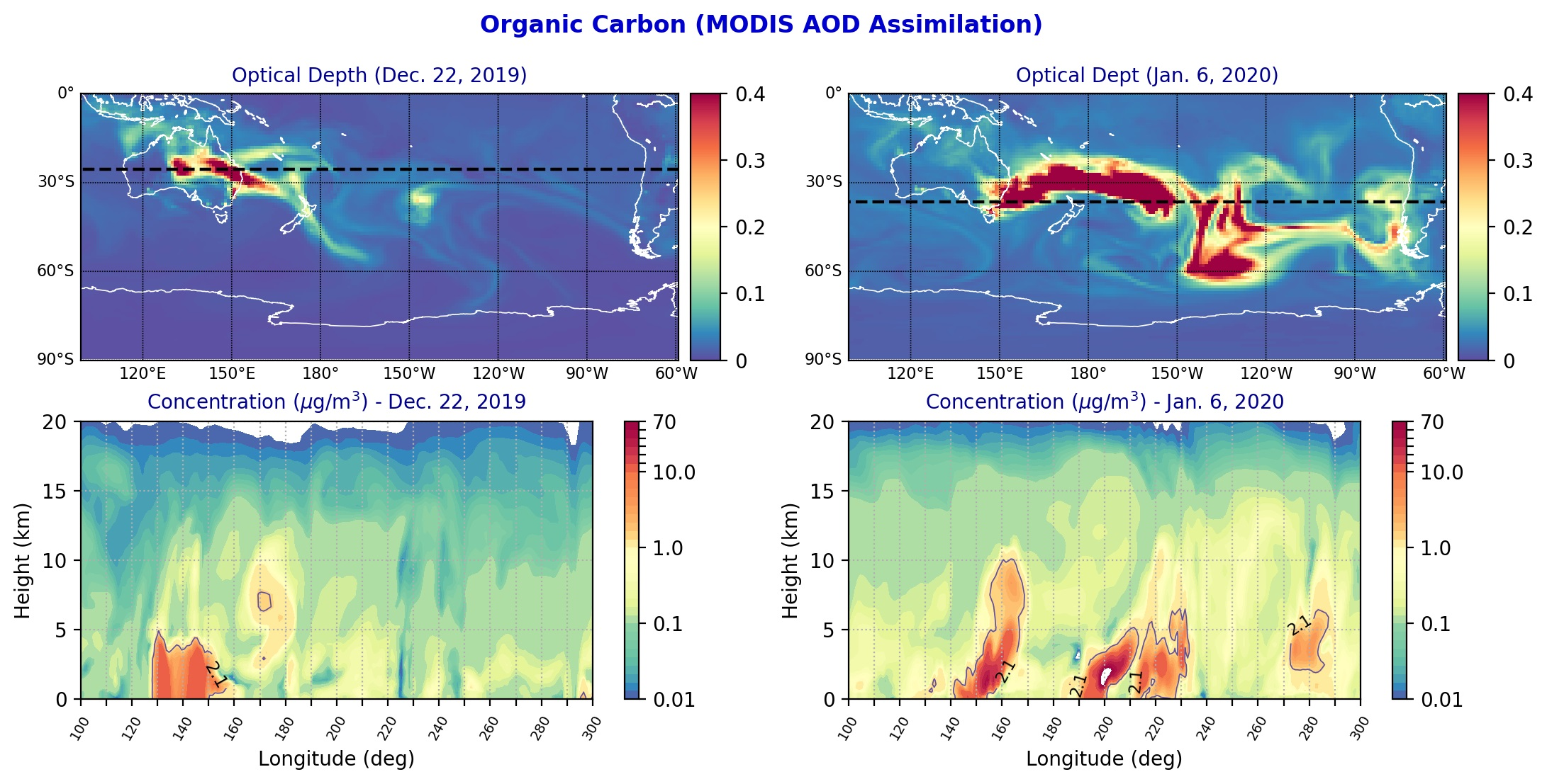
2.1. Performances of the Assimilation System

The first step will consist of validating the system based on assimilation diagnostics and by comparing the AOD analyses to independent observations at global scales. We first check the good functioning of the assimilation chain in terms of the assimilation diagnostics: OMF (observation minus forecasts) and OMA (observation minus analysis).
To evaluate the impact of MODIS AOD observations on the modelled fields, we analyse the performances of assimilation diagnostics in terms of OMA and OMF. Figure 1 shows the OMF and OMA histograms for all MODIS AOD measurements over the whole assimilation period (1 January 2018–31 December 2019). From this figure, we notice that the OMA histogram is narrower and its mean is closer to zero than that of OMF. This means that the bias between the observations and the model field is reduced due to the assimilation process. For all the year 2018, the mean value of OMF (OMA) is 0.024 (0.019) with a respective standard deviation of 0.19 (0.13). For the year 2019, these values are 0.022 (0.018) and 0.18 (0.13) for the mean values of OMF (OMA) and their standard deviations, respectively. This indicates that the analysis fields are closer to the observations than the forecast fields in terms of AOD.
Other statistics between the MODIS AOD observations and the forecasts on one hand, and between the MODIS AOD observations and the analyses in terms of correlation, bias and root mean square error (RMSE) are presented in Table 1.
The results of this assimilation diagnostics in terms of OMA and OMF show that the assimilated field is globally closer to the MODIS observations than the background field over the two year period of assimilation (1 January 2018–31 December 2019). These performances demonstrate that the MODIS assimilation improved the model field.

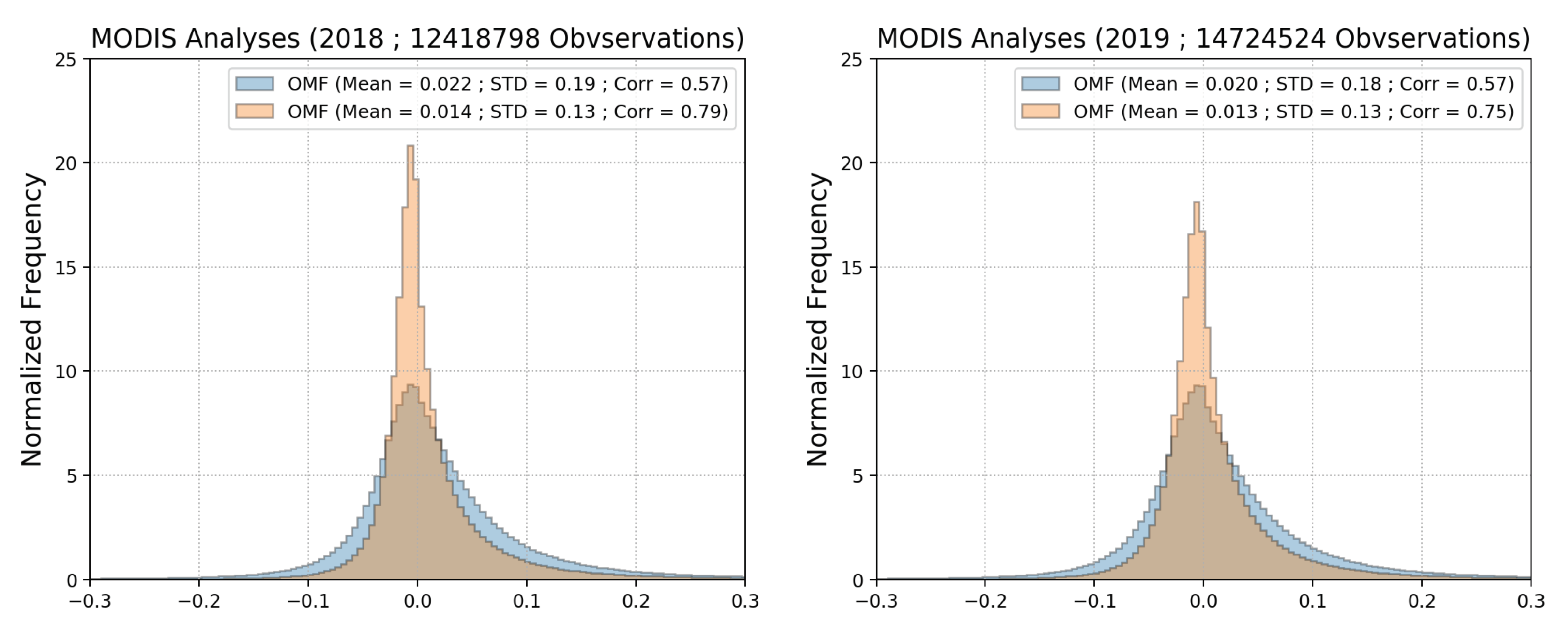
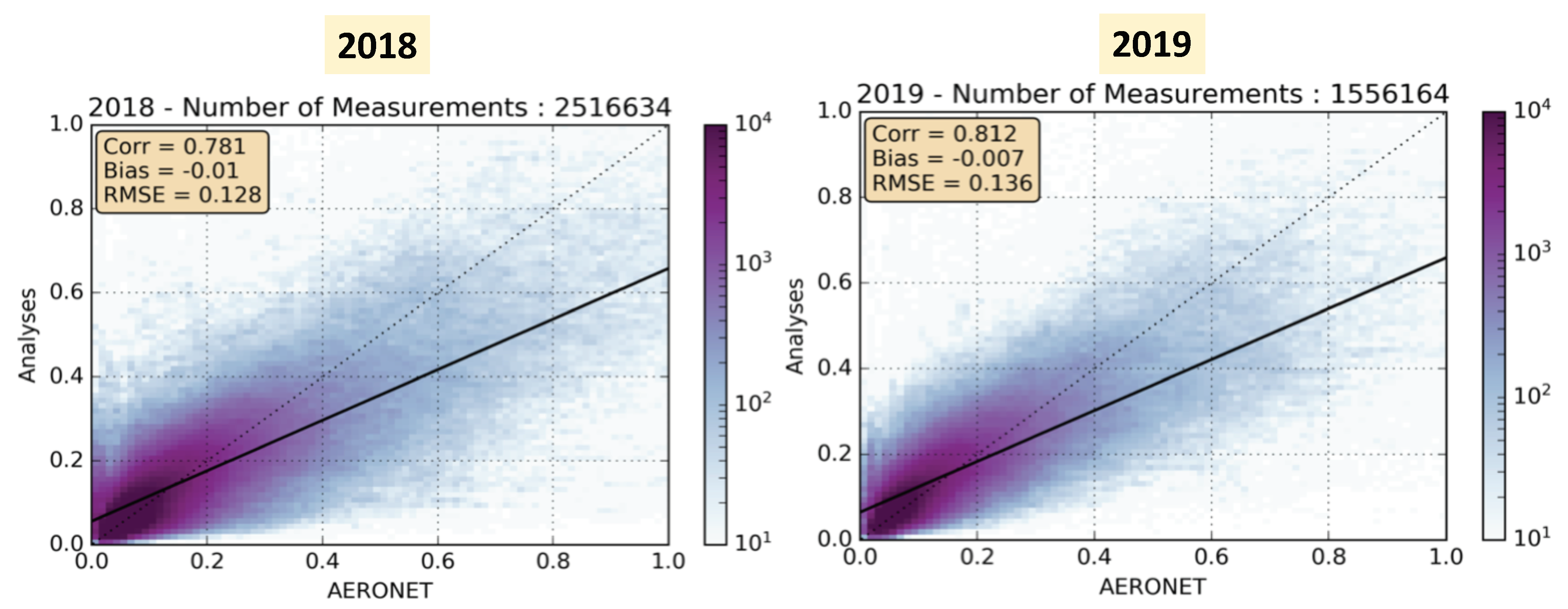
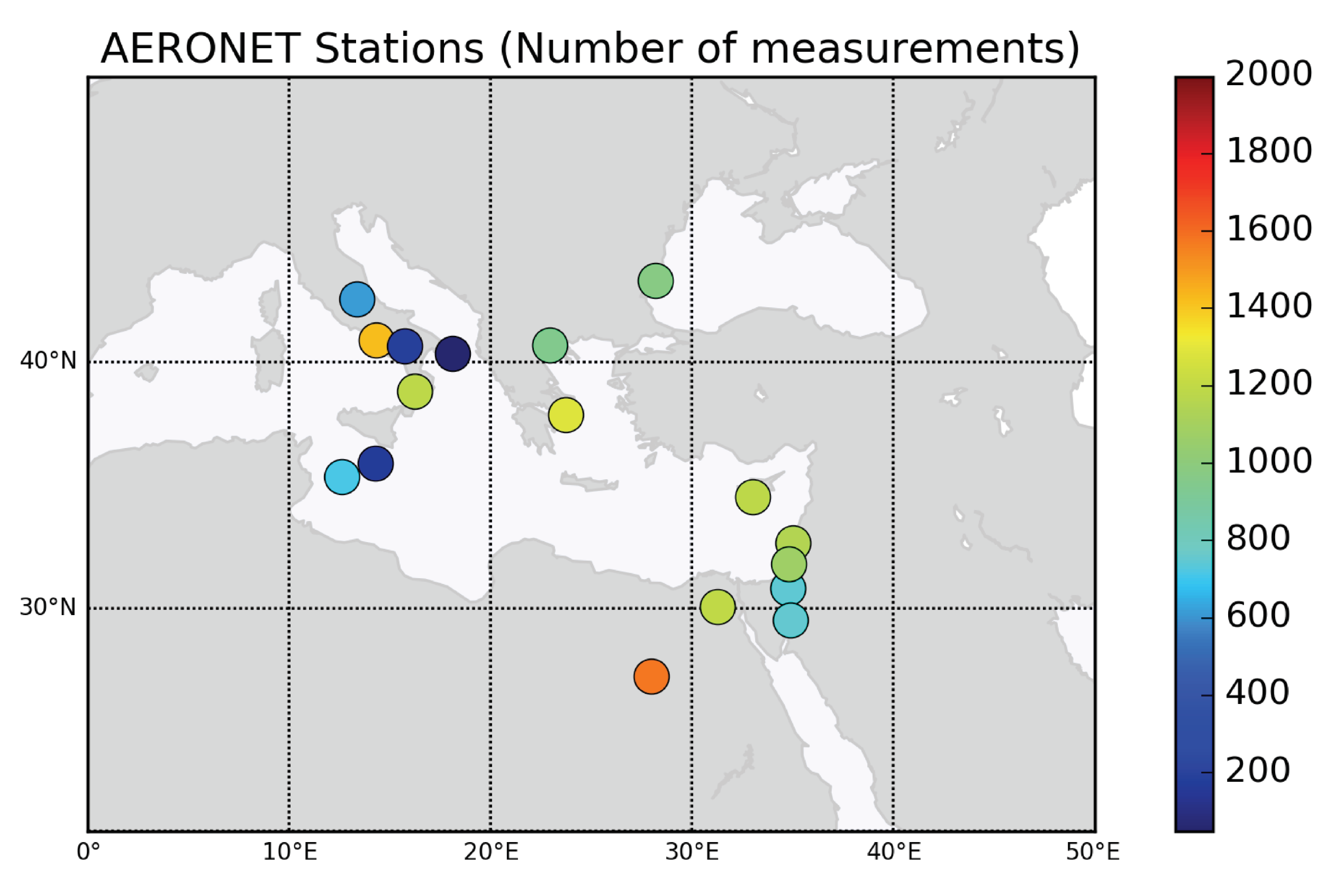
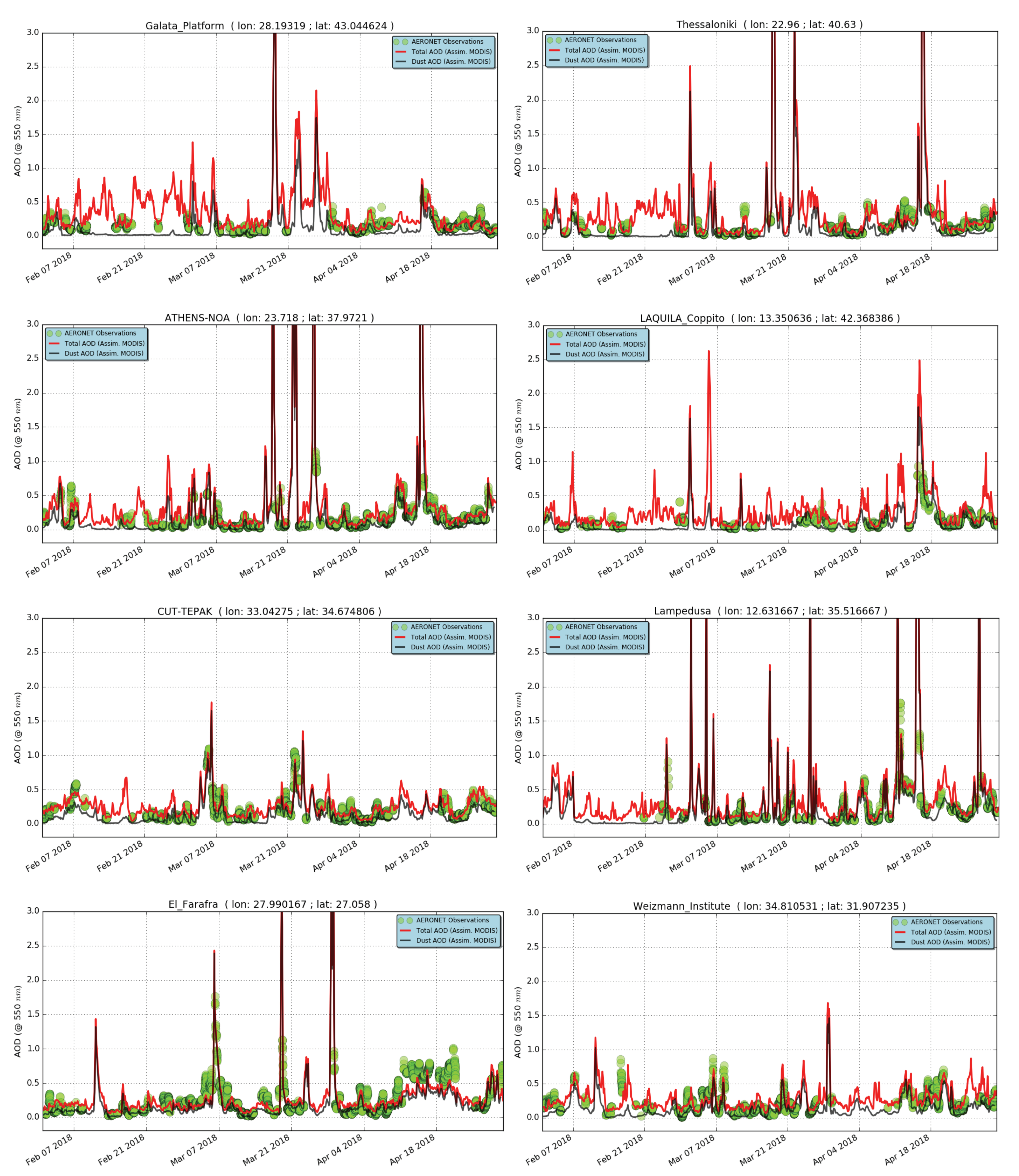
2.2. Comparison with AERONET In Situ Observations

In a second step, we validate the quality of the pre-operational assimilation chain in terms of AOD values using all available AERONET (Aerosol Robotic Network) ground-based observations over the globe within the whole assimilation period. The added value of MODIS AOD assimilated products with respect to the model free run has already been evidenced by comparison to many independent observations including SEVIRI (spinning enhanced visible and Infrared imager) geostationary, AERONET and in situ aircraft and balloon observations (see [26,57]).
The AERONET project is a global network of ground-based aerosol measurements. It uses CIMEL radiometers to measure the extinction of the direct solar radiation in the range of 340–1020 nm. AERONET provided long-term aerosol measurements for several aerosol studies and characterisation and validation of satellite observations. AERONET data are available at three levels: Level 1 (unfiltered), Level 1.5 (cloud filtered) and Level 2 (cloud filtered and quality assured). For more information on the AERONET project, the reader can refer to “https://aeronet.gsfc.nasa.gov/” (accessed on 30 March 2022).
Figure 2 shows the statistics in terms of correlation, bias and RMSE between the MODIS analyses versus available AERONET observations with respect to each measurement’s site over the two years of comparison 2018 and 2019. Generally, the correlation coefficient is greater than 0.7 for the majority of AERONET stations. Similarly, the bias and root mean square error between the assimilated product and the AERONET measurements are relatively low for the two years of comparison. Overall, we note that there is no systematic bias and that it can be positive or negative. The absolute value of the bias does not generally exceed 0.08 except over certain regions (Central Africa and South East Asia) where the bias value sometimes exceeds 0.1. This may be due to biomass fire emissions over the African continent or the anthropogenic activities in Asia which are not very well represented in the model. Note that Anderson et al. [58] report that the MODIS AODs retrieved over land have a much larger bias than the AODs retrieved from the oceans compared to AERONET in situ measurements for most of the sites located on the coast. This result is consistent with the difficulties encountered when characterizing land surfaces. It was also noted that the bias shows large variations between different coastal AERONET measurement sites, which likely reflects variations in coastal surface characteristics (e.g., [59,60]). In conclusion, the results presented in this figure illustrate the very good behaviour of the MOCAGE model using MODIS AOD data assimilation to better represent the AOD distribution at the global scale compared to the AERONET in situ observations over the two years of comparison.
In order to assess the overall behaviour of MODIS assimilated fields with respect to AERONET observations over the whole period of comparison, we represent in Figure 3 a scatter plot of AERONET AOD versus assimilated MODIS AOD for the two years of study, 2018 and 2019. The correlation between AERONET observations and the assimilated MODIS AOD output for the year of 2018 (2019) is 0.781 (0.812), whereas the bias is −0.01 (−0.007) and the RMSE is 0.128 (0.136). We note also that the AODs from the MODIS AOD assimilated field are overestimated for low AOD values (lower than 0.1). This is probably due to the observations of the stations located at high altitude, in agreement with other studies which indicate that the AOD over locations of high altitude is generally smaller than that over low altitude (e.g., [61,62]). This behaviour has also been reported recently by comparison of CALIOP (Cloud-Aerosol Lidar with Orthogonal Polarization) assimilated measurements onboard CALIPSO (Cloud-Aerosol Lidar and Infrared Pathfinder Satellite Observation) in terms of extinction coefficient to AERONET in situ observations [27].

3. Major Desert Dust Outbreak over Eastern Mediterranean: March 2018

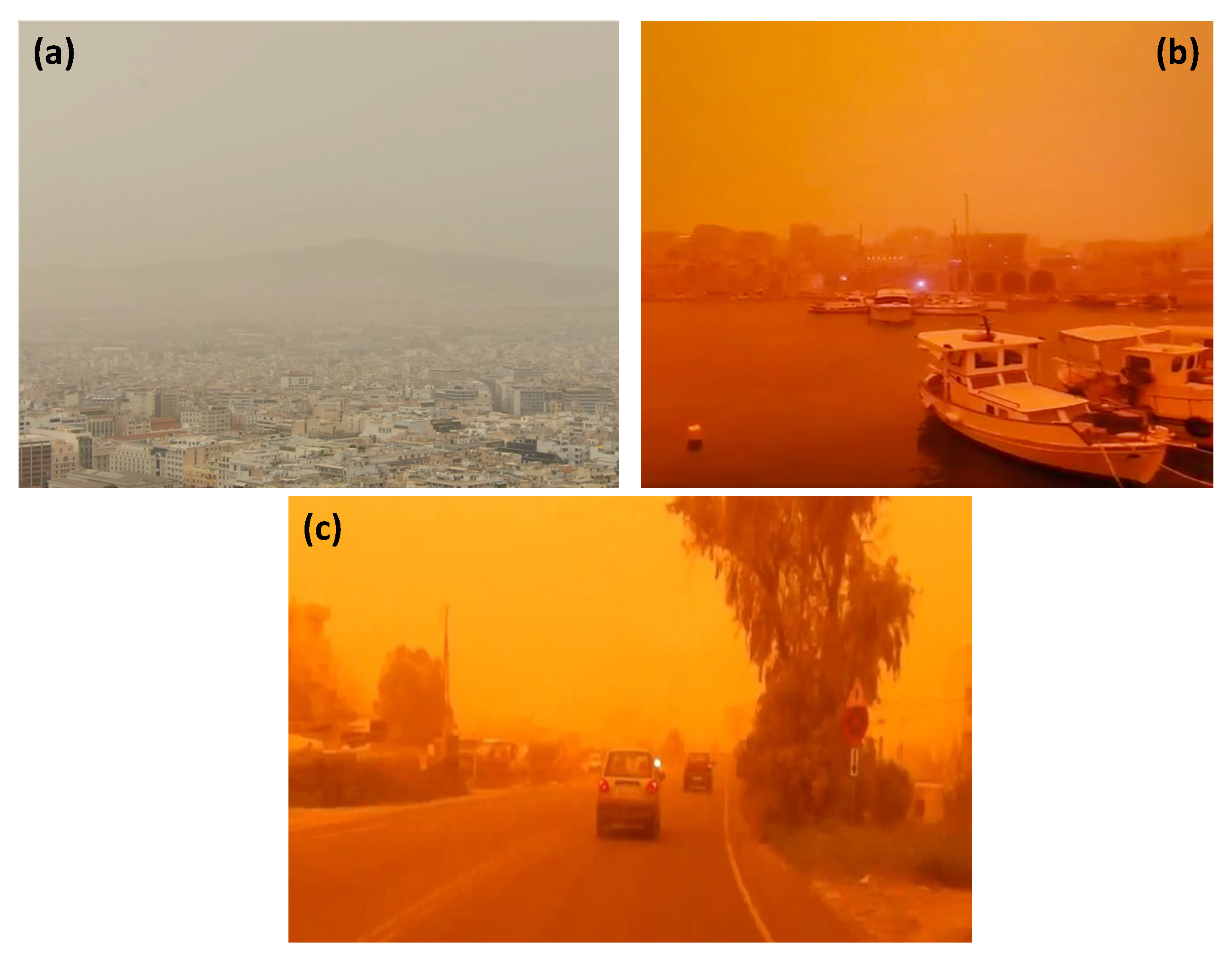
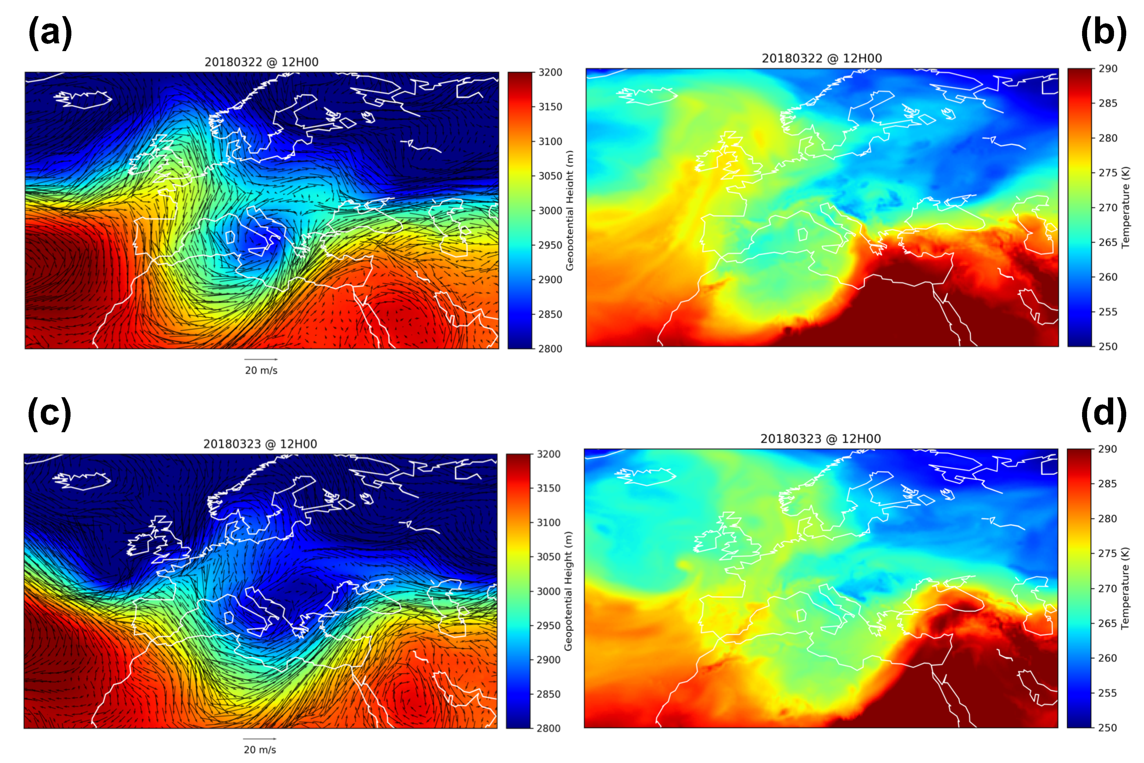
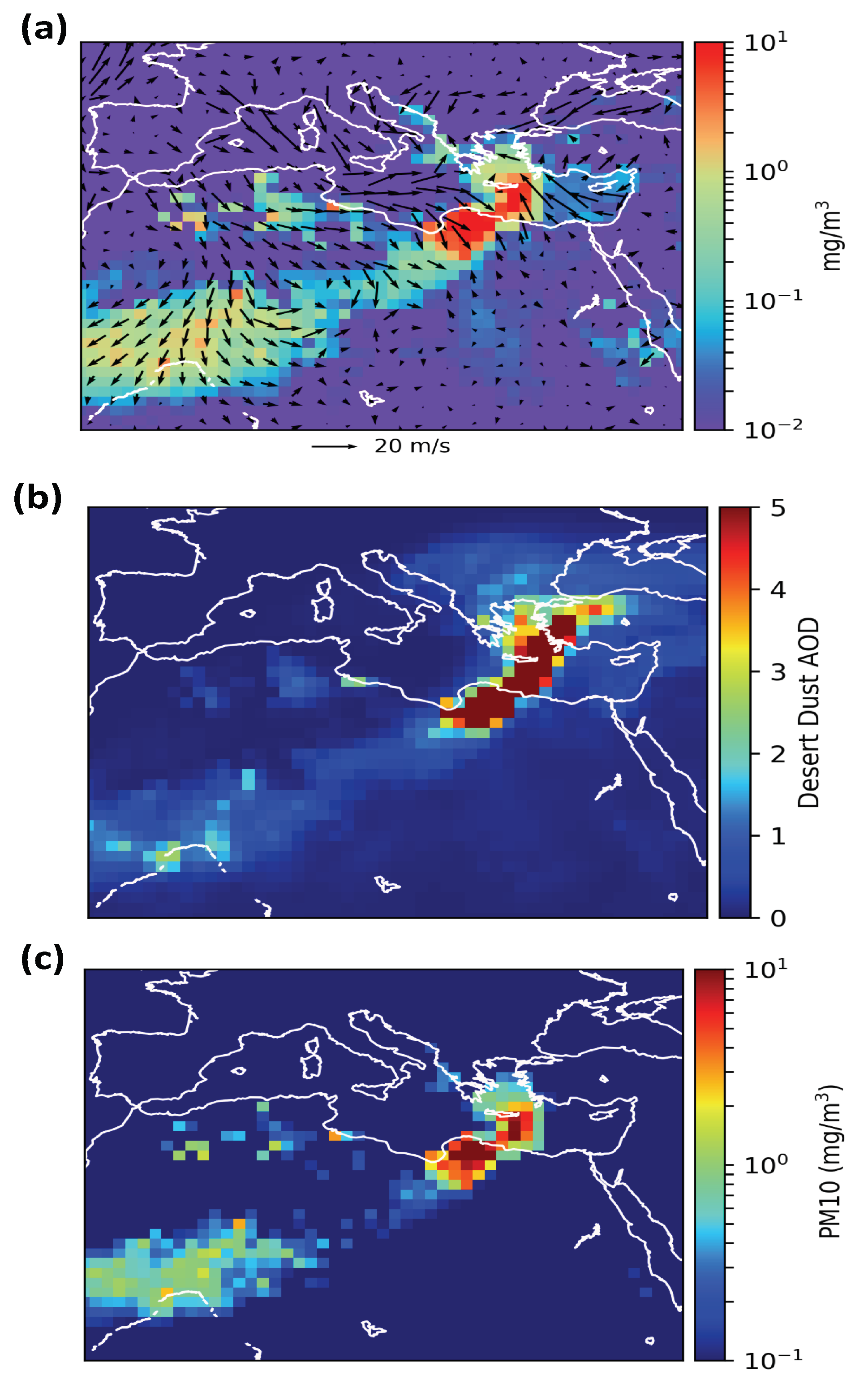
3.1. Desert Dust Event over Greece on 22 March 2018

Desert dust has direct and indirect impacts on several areas including human health, civil aviation, air quality, visibility, solar energy, agriculture and the global ecological system (e.g., [63,64,65]). It is considered to be one of the aerosol components that has a significant impact on the climate system’s variability [2] as well as on the deterioration of the air quality at regional and local scales [66]. It is also considered to be an important factor that affects meteorological weather by influencing atmospheric dynamics, clouds and precipitation formation [2].
On 22 March, 2018, huge amounts of desert dust were transported from Libya to Greece and the Eastern Mediterranean due to a localized depression in the central Mediterranean. This event had a considerable impact on the whole region, particularly on the island of Crete. It was therefore widely reported by various media (see e.g., https://watchers.news/2018/03/23/severe-dust-storm-hits-crete-greece/ accessed on 10 April 2022).
The consequences were very important since the air was completely saturated by desert dust particles and the visibility was very poor.
This episode represents a dust transport situation over the eastern part of the Mediterranean Basin, including Greece and Egypt. This episode clearly captures the transport patterns caused by the omega blocking (see the description of the synoptic situation later), with dust fluxes penetrating from the north-west of Africa to the eastern part of the Mediterranean Sea, including Greece, Egypt and the Arabian Peninsula.
Figure 4 shows some pictures illustrating the atmospheric situation over different locations in Greece during this desert dust outbreak event. Different media reported that a thick layer of Saharan sand spread on the island of Crete on the afternoon of 22 March, reducing the visibility at Heraklion airport to about 600 m. In some parts of the island, like Chania, the desert dust was mixed with the smoke from local wildfires, making the air highly saturated and unbreathable.
In order to learn more about the dynamics and the mechanisms of this desert dust event, we analyse the synoptic parameters in terms of geopotential and temperature at 700 hPa. This level has been widely used to diagnose the synoptic situation because it generally corresponds to the average desert dust transportation level (e.g., [67,68]).
Figure 5 illustrates the synoptic situation including the geopotential height in m with wind flow in m·s 1 (Figure 5a,c) and temperature in K (Figure 5b,d) at 700 hPa for the two days 22 and 23 March 2018 during the desert dust outbreak event. The meteorological data were taken from the ERA5 reanalysis (e.g., [69]). The Saharan dust event at a continental scale began on 22 March 2018 over Morocco and the south of Algeria in the north-west of the African continent. This day was also characterized by a cyclonic situation that developed over Balearic Islands and Italy which favours a cold front over this region and reached North Africa. The eastward movement of the cold front along the North African coast is illustrated in the contours of the geopotential height. The temperature field at the same day show almost the same behaviour as the geopotential height. A strong temperature gradient and baroclinic atmosphere at 700 hPa were seen in east and southeast of Greece, which are signs of the presence of a front over this region. Furthermore, the cold advection is associated with an intense temperature gradient at the west of the low-pressure centre. At this level, a trough that stretched over northern Europe reduced the temperature, while over the east of the Mediterranean Basin and the Arabian Peninsula high geopotential height dominated and the temperature was significantly higher. The cold front traversing through Italy was accompanied by strong southeasterlies ahead (>25 m·s 1 ). These strong winds were the trigger of an intense dust storm on this day.
On 23 March 2018, the core of the low-pressure moved north-east with intensification of the intensity. At the 700 hPa pressure level, a cut-off low centre prevailed over Greece, displaying similar characteristics as during 22 March but with higher intensity in its core. In addition, this trough facilitated a strong pressure gradient and the formation of a deep, low pressure accompanied by a front extended to the north-west of Turkey. A strong temperature gradient and baroclinic atmosphere were seen in the east of Egypt extending to the north of Turkey (see Figure 5d). On this day, the desert dust outbreak was particularly intense over Egypt and the east part of the Mediterranean Basin.

3.2. Comparison to AERONET Observations

In this section we highlight the performances and the effectiveness of the assimilation chain in reproducing the time evolution of the aerosol concentration during the desert dust event. We use Version 3 of AOD L2 observations issued from the AERONET network collected from the stations concerned by the desert dust outbreak on 22 March 2018 over the eastern Mediterranean.
The locations as well as the number of AOD measurements for each considered station used for the evaluation of MODIS AOD assimilation run between February and April 2018 are presented in Figure 6. Seventeen AERONET stations are located within the desert dust transport event and are considered for the comparison.
Assimilated field hourly available during the comparison period at the 550 nm wavelength is interpolated into the AERONET time measurements. In order to make the AOD wavelengths of different stations consistent with those of the assimilated field, AERONET measurements are interpolated in a logarithmic scale at 550 nm using all available neighbouring wavelengths (440, 500, 675 and 870 nm). Figure 7 presents the time evolution of the assimilated field compared to AERONET measurements in terms of AOD for the period February–April 2018 for selected stations. The time evolution of the AOD from the assimilated field is generally consistent with that of AERONET observations over the whole period of comparison. This comparison is considered as a kind of validation of the assimilated product in terms of AOD before, during and after the dust event in the same way already done by, e.g., Sič et al. [26] and El Amraoui et al. [27]. Around the period of the desert dust event, the stations located in the west recorded the event earlier than the stations located in the east in accordance with the synoptic evolution of the geopotential height and the temperature (see Figure 5). The AOD from the assimilation chain highlights very clearly the desert dust event with relatively high AOD values around 22 March 2018.
The scores in terms of correlation, bias and RMSE between the MODIS assimilation run and the AERONET in situ measurements for all the stations of comparison are given in Table 2. Generally, the agreement between MODIS analyses issued from the assimilation chain and AERONET data is very good over the three months of comparison.
In order to have an idea about the spatial extension as well as the evolution of this event, we show in Figure 8 maps in terms of the longitude–latitude of different parameters issued from the pre-operational chain during the desert dust event on 22 March 2018 at 12:00. These parameters concern the surface desert dust concentration (Figure 8a), the desert dust AOD (Figure 8b) and surface PM10 concentration (Figure 8c). This figure highlights very clearly the signature of the desert dust over the eastern mediterranean with a similar pattern for all desert dust parameters shown in the figure (desert dust of both surface concentration and AOD as well as surface PM10).

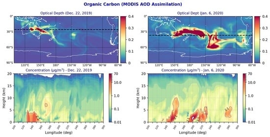
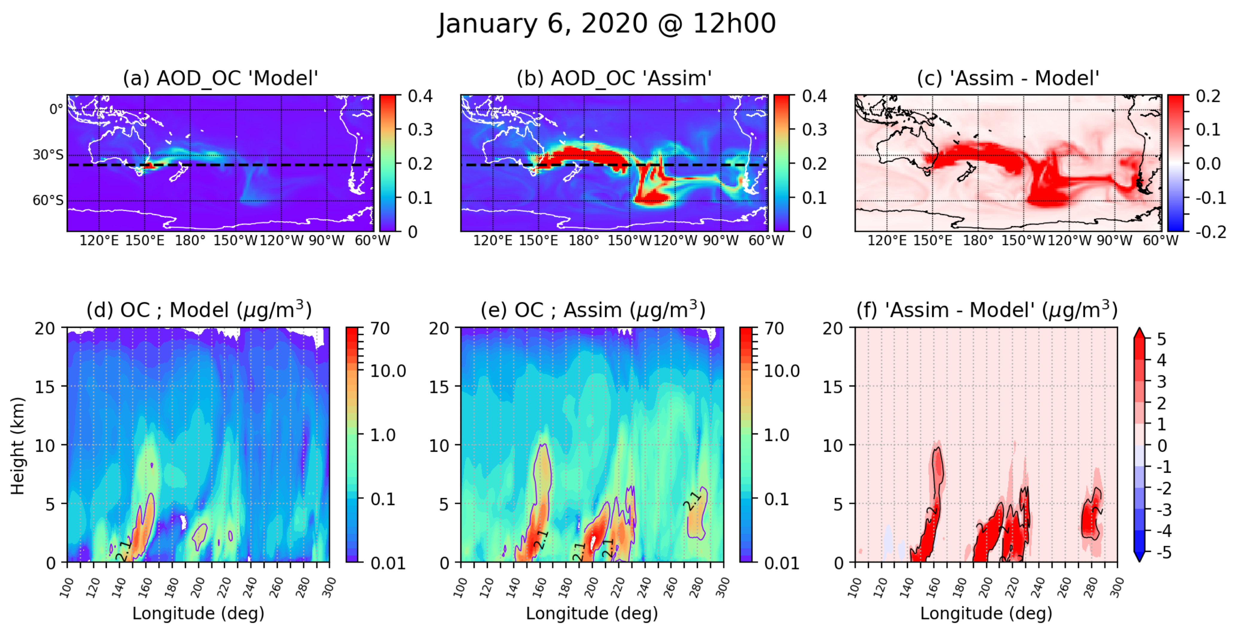
4. Australian Wildfires: November 2019

Wildfire emissions have negative impacts on air quality, visibility and generally on ecosystems at a large scale [70]. Forest fires are a key component of terrestrial socio-ecological systems (e.g., [71]). They produce a range of pollutants in terms of particulate matter, carbonaceous and nitrogenous species as well as ozone precursors (e.g., [72]). All these pollutants have an impact on atmospheric chemistry, air quality at local and regional scales as well as on global pollution (e.g., [73]). Forest fire emissions, unlike industrial emissions, are episodic in both space and time. Their effects on air quality and human health can occur in the short and long term (e.g., [74]). Forest fires are unavoidable and play an essential role in many terrestrial ecosystems. Nevertheless, the smoke produced by these fires is of considerable societal concern (e.g., [75]). Therefore, research and environmental policy that addresses fire issues must ensure a balance that will ensure the proper functioning of ecosystems, taking into account all the links with other sectors, and on the other hand maintaining and preserving air quality and thus avoiding any pollution risk in order to protect human health (e.g., [76]).
Between July 2019 and February 2020, Australia experienced huge fires with an unprecedented amplitude and a fairly large spatial extent (of the order of 97,000 km 2 ). The consequences of these fires are significant both for local biodiversity and for regional air quality and pollution.
In this section we evaluate the added value of the assimilation chain compared to the free model predictions to better document this fire event.
First, we will evaluate the assimilated run compared to the MOCAGE free model run in terms of vertical profiles during the Australian fire event. Figure 9a represents a set of trajectories from the CALIOP instrument collected during 6 January 2020 over the Australian region. The colour code refers to the number of all the ascending and descending profiles collected during that day. Figure 9b shows all vertical profiles corresponding to the trajectories of Figure 9a in terms of backscatter coefficients (in m 1 · sr 1 ), and Figure 9c shows the same vertical profiles in terms of the backscatter coefficient from the free model run. The comparison between the three products shows that the free model field produces the same structures as for the CALIOP measurements in terms of backscatter coefficient but the values are systematically underestimated. The assimilation of MODIS AOD shown in Figure 9d highlights a clear improvement of the model free run field. Figure 9d shows that the assimilation field reproduces the areas of high backscatter coefficient values. Globally, the assimilation run is closer to the CALIOP measurements than the free run model field. This comparison clearly shows that the assimilation of MODIS AOD significantly improves the outputs of the MOCAGE model. Figure 9e represents the mean vertical profiles corresponding to the ratios: CALIOP MOCAGE and CALIOP ASSIMILATION , respectively, with their respective standard deviations (Figure 9f). The mean vertical profile of CALIOP ASSIMILATION is closer to 1 than that of the ratio CALIOP MOCAGE . Moreover, the standard deviation of the ratio including the assimilation product is small than that of the ratio including MOCAGE. This confirms again that the MODIS assimilated field is close to the CALIOP independent data in terms of backscatter coefficient than that of the model.) Figure 9 shows that the assimilated product allows a better description of the Australian fire event compared to the model outputs.
Hereafter, we will document this event using the assimilated product. Figure 10 shows an illustration of the signature of the Australian wildfire in terms of both optical depth and concentration of OC. The OC is considered as one of the important tracers of aerosol smoke from fires (e.g., [77,78]). Jaffe et al. [79] reported that OC is considered as a primary component of the particulate matter emitted by fires. They also indicated that the relationship of OC with fire biomass burned in all regions is statistically significant. Figure 10a,b show the OC optical depth from the model and the MODIS assimilated product, respectively. The Australian fire signature is presented in the aerosol optical depth of OC in both the MOCAGE model as well as in the assimilated product. However, the MOCAGE model underestimates the OC AOD values especially over eastern Australia where the spread of the fire plume is well represented in the assimilated field with a much improved signature. The OC aerosol optical depth from the assimilated product shows a much more pronounced fire signature than that from the MOCAGE model. The difference between the two products presented in Figure 10c highlights the improvement of the assimilated field despite the fact that quantitatively the plume is represented in the model product. The pre-operational assimilation chain product provides a better description both qualitatively and quantitatively of the Australian fire smoke spread than the model product.
Several studies indicate that OC can be considered as a tracer for the detection of fire propagation (e.g., [79]). The threshold value above which the OC concentrations can be considered as high within a fire plume is 2.1 μ g·m 3 (see, e.g., [80]). Figure 10d shows a zonal vertical cross-section (longitude versus altitude) along the latitude line of 37.5 S (represented by a thick line in the figure) between 100 E and 60 W (noted 300 in the figure) and between 0 and 20 km in the vertical.
The high concentrations of OC as delimited by the 2.1 μ g·m 3 contour are present in the model free field at about the longitude 150 E and extend from the surface up to about 10 km and propagate upwards in the direction of the plume to the east. The assimilated product shows much more accentuated structures with several plumes containing high concentrations of OC. The plume located at the longitude 150 S in the model field is also present within the assimilated product but with higher concentrations and with an altitude which exceeds that recorded in the model field (∼10 km). In addition to this plume, the assimilated product records two other plumes, the first one around the longitude 190 (170 W) reaching 5 km, and the second around the longitude 220 (140 W) with a vertical extension exceeding 5 km. These two plumes with high OC concentrations are totally missed in the model field even if their signature exists with very low OC concentrations. This shows that even if the AOD is an integrated value over the whole atmospheric column, its assimilation allows to adjust the vertical distribution of the different aerosol types. These findings clearly illustrate the ability of the assimilation chain to predict well the evolution of the fire plume compared to the results of the free model field.

5. Conclusions

In this study we presented an assimilation system that operates in a pre-operational mode on a daily basis. It uses the assimilation of AOD observations from the MODIS (Moderate Resolution Imaging Spectroradiometer) instrument onboard both Terra and Aqua satellites at the global scale with a resolution of 1 × 1 . We validated this assimilation chain over a two-year period, 2018 and 2019, using the assimilation diagnostics in terms of OMF and OMA as well as the independent AOD data from the AERONET network. The added value of the fields resulting from this assimilation chain compared to those resulting from the free model run without assimilation was demonstrated and quantified. We also highlighted the capacity of this chain to predict and document extreme events such as desert dust transport or biomass wildfire propagation.
This chain has been improved since 2020 with the addition of other observations in the assimilation system in terms of AOD observations from the VIIRS (Visible Infrared Imaging Radiometer Suite) instrument as well as lidar profiles from the MPL (mini pulse lidars) network located over France and part of the E-PROFILE network of the European Environment Agency. The inclusion of these two sets of data in the chain has been validated. Improvements even in the scores compared to the AERONET data have been noticed. The work presented in this paper constitutes the basis of the operational chain of Météo-France for aerosol assimilation. This chain has been in operational mode since January 2022.

Author Contributions

Formal analysis, L.E.A. and F.C.; Investigation, L.E.A.; Methodology, L.E.A., M.P., V.G., F.C. and M.B.; Project administration, L.E.A.; Supervision, M.P., V.G., F.C. and M.B.; Validation, M.P., V.G., F.C. and M.B.; Visualization, F.C.; Writing—original draft, L.E.A.; Writing—review & editing, L.E.A., M.P., V.G., F.C. and M.B. All authors have read and agreed to the published version of the manuscript.

Funding

This research received no external funding.

Institutional Review Board Statement

Not applicable.

Informed Consent Statement

Not applicable.

Data Availability Statement

The MODIS data are available at: https://ladsweb.modaps.eosdis.nasa.gov/archive/allData/61, accessed on 5 Mrach 2022. The AERONET data are available at: https://aeronet.gsfc.nasa.gov, accessed on 5 Mrach 2022. The CALIOP data are available at: https://www.icare.univ-lille.fr/asd-content/calipso, accessed on 5 Mrach 2022. The MODIS assimilation products are available from the authors upon reasonable request.

Acknowledgments

This work is funded in France by the Centre National de Recherches Météorologiques (CNRM) of Météo-France and the Centre National de Recherches Scientifiques (CNRS). We would also like to thank ECMWF for providing ERA5 analyses, NASA for providing MODIS and AERONET data and the ICARE, the French atmospheric composition database (CNES and CNRS-INSU), for providing CALIOP data. We also would like to thank all the reviewers as well as the Editor for their valuable comments which were very helpful in improving the paper.

Conflicts of Interest

The authors declare no conflict of interest.

References

  1. Mahowald, N.; Luo, C.; Del Corral, J.; Zender, C.S. Interannual variability in atmospheric mineral aerosols from a 22-year model simulation and observational data. J. Geophys. Res. 2003, 108, 4352. [Google Scholar] [CrossRef] [Green Version]
  2. IPCC. Intergovernmental Panel on Climate Change, Climate Change 2013: The Physical Science Basis, Contribution of Working Group I to the Fifth Assessment Report of the Intergovernmental Panel on Climate Change; Stocker, T.F., Qin, D., Plattner, G.-K., Tignor, M.M.B., Allen, S.K., Boschung, J., Nauels, A., Xia, Y., Bex, V., Midgley, P.M., Eds.; Cambridge University Press: Cambridge, UK, 2013. [Google Scholar]
  3. Van der Werf, G.R.; Randerson, J.T.; Giglio, L.; Collatz, G.; Mu, M.; Kasibhatla, P.S.; Morton, D.C.; DeFries, R.; Jin, Y.V.; van Leeuwen, T.T. Global fire emissions and the contribution of deforestation, savanna, forest, agricultural, and peat fires (1997–2009). Atmos. Chem. Phys. 2010, 10, 11707–11735. [Google Scholar] [CrossRef] [Green Version]
  4. Jing, B.; Peng, C.; Wang, Y.; Liu, Q.; Tong, S.; Zhang, Y.; Ge, M. Hygroscopic properties of potassium chloride and its internal mixtures with organic compounds relevant to biomass burning aerosol particles. Sci. Rep. 2017, 7, 43572. [Google Scholar] [CrossRef] [PubMed] [Green Version]
  5. IPCC. Intergovernmental Panel on Climate Change, Climate Change 2001: The scientific Basis. Contribution of Working Group I to the Third Assessment Report of the Intergovernmental Panel on Climate Change; Houghton, J.T., Ding, Y., griggs, D.J., Noguer, M., van der Linden, P.J., Dai, X., Maskell, K., Johnson, C.A., Eds.; Cambridge University Press: Cambridge, UK; New York, NY, USA, 2001. [Google Scholar]
  6. Evangelista, H.; Maldonado, J.; Godoi, R.; Pereira, E.; Koch, D.; Tanizaki-Fonseca, K.; Van Grieken, R.; Sampaio, M.; Setzer, A.; Alencar, A.; et al. Sources and transport of urban and biomass burning aerosol black carbon at the South–West Atlantic Coast. J. Atmos. Chem. 2007, 56, 225–238. [Google Scholar] [CrossRef] [Green Version]
  7. Zielinski, T.; Bolzacchini, E.; Cataldi, M.; Ferrero, L.; Graßl, S.; Hansen, G.; Mateos, D.; Mazzola, M.; Neuber, R.; Pakszys, P.; et al. Study of Chemical and Optical Properties of Biomass Burning Aerosols during Long-Range Transport Events toward the Arctic in Summer 2017. Atmosphere 2020, 11, 84. [Google Scholar] [CrossRef] [Green Version]
  8. Crutzen, P.J.; Andreae, M.O. Biomass burning in the tropics: Impact on atmospheric chemistry and biogeochemical cycles. Science 1990, 250, 1669–1678. [Google Scholar] [CrossRef]
  9. Reid, J.; Koppmann, R.; Eck, T.; Eleuterio, D. A review of biomass burning emissions part II: Intensive physical properties of biomass burning particles. Atmos. Chem. Phys. 2005, 5, 799–825. [Google Scholar] [CrossRef] [Green Version]
  10. Milton, S.; Greed, G.; Brooks, M.; Haywood, J.; Johnson, B.; Allan, R.; Slingo, A.; Grey, W. Modeled and observed atmospheric radiation balance during the West African dry season: Role of mineral dust, biomass burning aerosol, and surface albedo. J. Geophys. Res. 2008, 113. [Google Scholar] [CrossRef] [Green Version]
  11. Lisok, J.; Rozwadowska, A.; Pedersen, J.; Markowicz, K.; Ritter, C.; Kaminski, J.W.; Struzewska, J.; Mazzola, M.; Udisti, R.; Becagli, S.; et al. Radiative impact of an extreme Arctic biomass-burning event. Atmos. Chem. Phys. 2018, 18, 8829–8848. [Google Scholar] [CrossRef] [Green Version]
  12. Pani, S.K.; Lin, N.H.; Chantara, S.; Wang, S.H.; Khamkaew, C.; Prapamontol, T.; Janjai, S. Radiative response of biomass-burning aerosols over an urban atmosphere in northern peninsular Southeast Asia. Sci. Total Environ. 2018, 633, 892–911. [Google Scholar] [CrossRef]
  13. Martins, L.D.; Hallak, R.; Alves, R.C.; de Almeida, D.S.; Squizzato, R.; Moreira, C.A.; Beal, A.; da Silva, I.; Rudke, A.; Martins, J.A. Long-range transport of aerosols from biomass burning over southeastern South America and their implications on air quality. Aerosol. Air Qual. Res. 2018, 18, 1734–1745. [Google Scholar] [CrossRef] [Green Version]
  14. Liu, T.; Marlier, M.E.; DeFries, R.S.; Westervelt, D.M.; Xia, K.R.; Fiore, A.M.; Mickley, L.J.; Cusworth, D.H.; Milly, G. Seasonal impact of regional outdoor biomass burning on air pollution in three Indian cities: Delhi, Bengaluru, and Pune. Atmos. Environ. 2018, 172, 83–92. [Google Scholar] [CrossRef]
  15. Uranishi, K.; Ikemori, F.; Shimadera, H.; Kondo, A.; Sugata, S. Impact of field biomass burning on local pollution and long-range transport of PM2. 5 in Northeast Asia. Environ. Pollut. 2019, 244, 414–422. [Google Scholar] [CrossRef] [PubMed]
  16. Shao, Y.; Wyrwoll, K.H.; Chappell, A.; Huang, J.; Lin, Z.; McTainsh, G.H.; Mikami, M.; Tanaka, T.Y.; Wang, X.; Yoon, S. Dust cycle: An emerging core theme in Earth system science. Aeolian Res. 2011, 2, 181–204. [Google Scholar] [CrossRef]
  17. Zhang, X.X.; Sharratt, B.; Liu, L.Y.; Wang, Z.F.; Pan, X.L.; Lei, J.Q.; Wu, S.X.; Huang, S.Y.; Guo, Y.H.; Li, J.; et al. East Asian dust storm in May 2017: Observations, modelling, and its influence on the Asia-Pacific region. Atmos. Chem. Phys. 2018, 18, 8353–8371. [Google Scholar] [CrossRef] [Green Version]
  18. Edwards, D.P.; Emmons, L.K.; Hauglustaine, D.A.; Chu, D.A.; Gille, J.C.; Kaufman, Y.J.; Pétron, G.; Yurganov, L.N.; Giglio, L.; Deeter, M.N.; et al. Observations of carbon monoxide and aerosols from the Terra satellite: Northern Hemisphere variability. J. Geophys. Res. 2004, 109, 24202. [Google Scholar] [CrossRef]
  19. Yi, B.; Yang, P.; Baum, B.A. Impact of pollution on the optical properties of trans-Pacific East Asian dust from satellite and ground-based measurements. J. Geophys. Res. 2014, 119, 5397–5409. [Google Scholar] [CrossRef]
  20. King, M.D.; Kaufman, Y.J.; Tanré, D.; Nakajima, T. Remote Sensing of Tropospheric Aerosols from Space: Past, Present, and Future. Bull. Am. Meteor. Soc. 1999, 80, 2229–2259. [Google Scholar] [CrossRef] [Green Version]
  21. Aminou, D. MSG’s SEVIRI instrument. ESA Bull. 2002, 111, 15–17. [Google Scholar]
  22. Winker, D.M.; Pelon, J.R.; McCormick, M.P. CALIPSO mission: Spaceborne lidar for observation of aerosols and clouds. In Lidar Remote Sensing for Industry and Environment Monitoring III; Singh, U.N., Itabe, T., Lui, Z., Eds.; International Society for Optics and Photonics: Bellingham, WA, USA, 2003; Volume 4893, pp. 1–11. [Google Scholar]
  23. Textor, C.; Schulz, M.; Guibert, S.; Kinne, S.; Balkanski, Y.; Bauer, S.; Berntsen, T.; Berglen, T.; Boucher, O.; Chin, M.; et al. Analysis and quantification of the diversities of aerosol life cycles within AeroCom. Atmos. Chem. Phys. 2006, 6, 1777–1813. [Google Scholar] [CrossRef] [Green Version]
  24. Schutgens, N.; Miyoshi, T.; Takemura, T.; Nakajima, T. Applying an ensemble Kalman filter to the assimilation of AERONET observations in a global aerosol transport model. Atmos. Chem. Phys. 2010, 10, 2561–2576. [Google Scholar] [CrossRef] [Green Version]
  25. El Amraoui, L.; Attié, J.L.; Ricaud, P.; Lahoz, W.A.; Piacentini, A.; Peuch, V.H.; Warner, J.X.; Abida, R.; Barré, J.; Zbinden, R. Tropospheric CO vertical profiles deduced from total columns using data assimilation: Methodology and Validation. Atmos. Meas. Tech. 2014, 7, 3035–3057. [Google Scholar] [CrossRef] [Green Version]
  26. Sič, B.; El Amraoui, L.; Piacentini, A.; Marécal, V.; Emili, E.; Cariolle, D.; Prather, M.; Attié, J.L. Aerosol data assimilation in the chemical transport model MOCAGE during the TRAQA/ChArMEx campaign: Aerosol optical depth. Atmos. Meas. Tech. 2016, 9, 5535–5554. [Google Scholar] [CrossRef] [Green Version]
  27. El Amraoui, L.; Sič, B.; Piacentini, A.; Marécal, V.; Frebourg, N.; Attié, J.L. Aerosol data assimilation in the MOCAGE chemical transport model during the TRAQA/ChArMEx campaign: Lidar observations. Atmos. Meas. Tech. 2020, 13, 4645–4667. [Google Scholar] [CrossRef]
  28. Klumpp, A.; Ansel, W.; Klumpp, G.; Belluzzo, N.; Calatayud, V.; Chaplin, N.; Garrec, J.; Gutsche, H.; Hayes, M.; Hentze, H.; et al. EuroBionet: A Pan-European biomonitoring network for urban air quality assessment. Environ. Sci. Pollut. Res. 2002, 9, 199–203. [Google Scholar] [CrossRef] [PubMed]
  29. Guerreiro, C.B.; Foltescu, V.; De Leeuw, F. Air quality status and trends in Europe. Atmos. Environ. 2014, 98, 376–384. [Google Scholar] [CrossRef] [Green Version]
  30. Barrero, M.; Orza, J.; Cabello, M.; Cantón, L. Categorisation of air quality monitoring stations by evaluation of PM10 variability. Sci. Total Environ. 2015, 524, 225–236. [Google Scholar] [CrossRef]
  31. Baldasano, J.; Jorba, O.; Vivanco, M.; Palomino, I.; Querol, X.; Pandolfi, M.; Sanz, M. Caliope: An operational air quality forecasting system for the Iberian Peninsula, Balearic Islands and Canary Islands–first annual evaluation and ongoing developments. Adv. Sci. Res. 2008, 2, 89. [Google Scholar] [CrossRef]
  32. Stortini, M.; Arvani, B.; Deserti, M. Operational Forecast and Daily Assessment of the Air Quality in Italy: A Copernicus-CAMS Downstream Service. Atmosphere 2020, 11, 447. [Google Scholar] [CrossRef]
  33. Wagner, A.; Blechschmidt, A.M.; Bouarar, I.; Brunke, E.G.; Clerbaux, C.; Cupeiro, M.; Cristofanelli, P.; Eskes, H.; Flemming, J.; Flentje, H.; et al. Evaluation of the MACC operational forecast system-potential and challenges of global near-real-time modelling with respect to reactive gases in the troposphere. Atmos. Chem. Phys. 2015, 15, 14005. [Google Scholar] [CrossRef] [Green Version]
  34. Gupta, P.; Christopher, S.A.; Wang, J.; Gehrig, R.; Lee, Y.; Kumar, N. Satellite remote sensing of particulate matter and air quality assessment over global cities. Atmos. Environ. 2006, 40, 5880–5892. [Google Scholar] [CrossRef]
  35. Emili, E.; Barret, B.; Massart, S.; Le Flochmoen, E.; Piacentini, A.; El Amraoui, L.; Pannekoucke, O.; Cariolle, D. Combined assimilation of IASI and MLS observations to constrain tropospheric and stratospheric ozone in a global chemical transport model. Atmos. Chem. Phys. 2014, 14, 177–198. [Google Scholar] [CrossRef] [Green Version]
  36. Fisher, M.; Andersson, E. Developments in 4D-Var and Kalman Filtering; Technical Memorandum Research Department: Berkshire, UK, 2001; Volume 347. [Google Scholar]
  37. Semane, N.; Peuch, V.H.; El Amraoui, L.; Bencherif, H.; Massart, S.; Cariolle, D.; Attié, J.L.; Abida, R. An observed and analysed stratospheric ozone intrusion over the high Canadian Arctic UTLS region during the summer of 2003. Quart. J. Roy. Meteor. Soc. 2007, 133, 171–178. [Google Scholar] [CrossRef]
  38. El Amraoui, L.; Peuch, V.H.; Ricaud, P.; Massart, S.; Semane, N.; Teyssèdre, H.; Cariolle, D.; Karcher, F. Ozone loss in the 2002–2003 Arctic vortex deduced from the assimilation of Odin/SMR O3 and N2O measurements: N2O as a dynamical tracer. Quart. J. Roy. Meteor. Soc. 2008, 134, 217–228. [Google Scholar] [CrossRef]
  39. El Amraoui, L.; Semane, N.; Peuch, V.H.; Santee, M.L. Investigation of dynamical processes in the polar stratospheric vortex during the unusually cold winter 2004/2005. Geophys. Res. Lett. 2008, 35, L03803. [Google Scholar] [CrossRef]
  40. Rabier, F.; Bouchard, A.; Brun, E.; Doerenbecher, A.; Guedj, S.; Guidard, V.; Karbou, F.; Peuch, V.; El Amraoui, L.; Puech, D.; et al. The Concordiasi Project in Antarctica. Bull. Am. Meteor. Soc. 2010, 91, 69–86. [Google Scholar] [CrossRef]
  41. Bencherif, H.; El Amraoui, L.; Kirgis, G.; Leclair De Bellevue, J.; Hauchecorne, A.; Mzé, N.; Portafaix, T.; Pazmino, A.; Goutail, F. Analysis of a rapid increase of stratospheric ozone during late austral summer 2008 over Kerguelen (49.4S, 70.3E). Atmos. Chem. Phys. 2011, 11, 363–373. [Google Scholar] [CrossRef] [Green Version]
  42. El Amraoui, L.; Attié, J.L.; Semane, N.; Claeyman, M.; Peuch, V.H.; Warner, J.; Ricaud, P.; Cammas, J.P.; Piacentini, A.; Josse, B.; et al. Midlatitude stratosphere–troposphere exchange as diagnosed by MLS O3 and MOPITT CO assimilated fields. Atmos. Chem. Phys. 2010, 10, 2175–2194. [Google Scholar] [CrossRef] [Green Version]
  43. Claeyman, M.; Attie, J.L.; Peuch, V.H.; El Amraoui, L.; Lahoz, W.A.; Josse, B.; Ricaud, P.; von Clarmann, T.; Hopfner, M.; Orphal, J.; et al. A geostationary thermal infrared sensor to monitor the lowermost troposphere: O3 and CO retrieval studies. Atmos. Meas. Tech. 2011, 4, 297–317. [Google Scholar] [CrossRef] [Green Version]
  44. Payra, S.; Ricaud, P.; Abida, R.; El Amraoui, L.; Attié, J.L.; Rivière, E.; Carminati, F.; Clarmann, T.V. Evaluation of water vapour assimilation in the tropical upper troposphere and lower stratosphere by a chemical transport model. Atmos. Meas. Tech. 2016, 9, 4355–4373. [Google Scholar] [CrossRef] [Green Version]
  45. Josse, B.; Simon, P.; Peuch, V.H. Radon global simulation with the multiscale chemistry trasnport model MOCAGE. Tellus 2004, 56, 339–356. [Google Scholar] [CrossRef]
  46. Teyssèdre, H.; Michou, M.; Clark, H.L.; Josse, B.; Karcher, F.; Olivié, D.; Peuch, V.H.; Saint-Martin, D.; Cariolle, D.; Attié, J.L.; et al. A new tropospheric and stratospheric Chemistry and Transport Model MOCAGE-Climat for multi-year studies: Evaluation of the present-day climatology and sensitivity to surface processes. Atmos. Chem. Phys. 2007, 7, 5815–5860. [Google Scholar] [CrossRef] [Green Version]
  47. Bousserez, N.; Attié, J.L.; Peuch, V.H.; Michou, M.; Pfister, G.; Edwards, D.; Emmons, L.; Mari, C.; Barret, B.; Arnold, S.R.; et al. Evaluation of the MOCAGE chemistry transport model during the ICARTT/ITOP experiment. J. Geophys. Res. 2007, 112. [Google Scholar] [CrossRef] [Green Version]
  48. Lacressonnière, G.; Peuch, V.; Arteta, J.; Josse, B.; Joly, M.; Marécal, V.; Martin, D.; Déqué, M.; Watson, L. How realistic are air quality hindcasts driven by forcings from climate model simulations? Geosci. Model Dev. 2012, 5, 1565–1587. [Google Scholar] [CrossRef] [Green Version]
  49. Barré, J.; EL Amraoui, L.; Ricaud, P.; Lahoz, W.A.; Attié, J.L.; Peuch, V.H.; Josse, B.; Marécal, V. Diagnosing the transition layer at extratropical latitudes using MLS O3 and MOPITT CO analyses. Atmos. Chem. Phys. 2013, 13, 7225–7240. [Google Scholar] [CrossRef] [Green Version]
  50. Martet, M.; Peuch, V.H.; Laurent, B.; Marticorena, B.; Bergametti, G. Evaluation of long-range transport and deposition of desert dust with the CTM MOCAGE. Tellus B 2009, 61, 449–463. [Google Scholar] [CrossRef]
  51. Sič, B.; El Amraoui, L.; Marécal, V.; Josse, B.; Arteta, J.; Guth, J.; Joly, M.; Hamer, P. Modelling of primary aerosols in the chemical transport model MOCAGE: Development and evaluation of aerosol physical parameterizations. Geosci. Model Dev. 2015, 8, 381–408. [Google Scholar] [CrossRef] [Green Version]
  52. Guth, J.; Josse, B.; Marécal, V.; Joly, M.; Hamer, P. First implementation of secondary inorganic aerosols in the MOCAGE version R2.15.0 chemistry transport model. Geosci. Model Dev. 2016, 9, 137–160. [Google Scholar] [CrossRef] [Green Version]
  53. Kaiser, J.; Heil, A.; Andreae, M.; Benedetti, A.; Chubarova, N.; Jones, L.; Morcrette, J.J.; Razinger, M.; Schultz, M.; Suttie, M.; et al. Biomass burning emissions estimated with a global fire assimilation system based on observed fire radiative power. Biogeosciences 2012, 9, 527. [Google Scholar] [CrossRef] [Green Version]
  54. Courtier, P.; Freydier, C.; Geleyn, J.; Rabier, F.; Rochas, M. The ARPEGE project at Météo France. In Atmospheric Models; ECMWF Workshop on Numerical Methods: Reading, UK, 1991; Volume 2, pp. 193–231. [Google Scholar]
  55. Bilal, M.; Qiu, Z.; Campbell, J.R.; Spak, S.N.; Shen, X.; Nazeer, M. A new MODIS C6 Dark Target and Deep Blue merged aerosol product on a 3 km spatial grid. Remote Sens. 2018, 10, 463. [Google Scholar] [CrossRef] [Green Version]
  56. Daley, R. Atmospheric Data Analysis; Number 2; Cambridge University Press: Cambridge, UK, 1993. [Google Scholar]
  57. Sič, B. Amélioration de la Représentation des Aérosols dans un Modèle de Chimie-Transport: Modélisation et Assimilation de Données. Ph.D. Thesis, Université de Toulouse, Université Toulouse III-Paul Sabatier, Toulouse, France, 2014. [Google Scholar]
  58. Anderson, J.C.; Wang, J.; Zeng, J.; Leptoukh, G.; Petrenko, M.; Ichoku, C.; Hu, C. Long-term statistical assessment of Aqua-MODIS aerosol optical depth over coastal regions: Bias characteristics and uncertainty sources. Tellus B Chem. Phys. Meteorol. 2013, 65, 20805. [Google Scholar] [CrossRef]
  59. Bennouna, Y.; Cachorro, V.; Toledano, C.; Berjón, A.; Prats, N.; Fuertes, D.; Gonzalez, R.; Rodrigo, R.; Torres, B.; de Frutos, A. Comparison of atmospheric aerosol climatologies over southwestern Spain derived from AERONET and MODIS. Remote Sens. Environ. 2011, 115, 1272–1284. [Google Scholar] [CrossRef]
  60. Remer, L.; Mattoo, S.; Levy, R.; Munchak, L. MODIS 3 km aerosol product: Algorithm and global perspective. Atmos. Meas. Tech. 2013, 6, 1829–1844. [Google Scholar] [CrossRef] [Green Version]
  61. Toledano, C.; González, R.; Fuertes, D.; Cuevas, E.; Eck, T.F.; Kazadzis, S.; Kouremeti, N.; Gröbner, J.; Goloub, P.; Blarel, L.; et al. Assessment of Sun photometer Langley calibration at the high-elevation sites Mauna Loa and Izaña. Atmos. Chem. Phys. 2018, 18, 14555–14567. [Google Scholar] [CrossRef] [Green Version]
  62. Wang, Y.; Yuan, Q.; Li, T.; Shen, H.; Zheng, L.; Zhang, L. Evaluation and comparison of MODIS Collection 6.1 aerosol optical depth against AERONET over regions in China with multifarious underlying surfaces. Atmos. Environ. 2019, 200, 280–301. [Google Scholar] [CrossRef] [Green Version]
  63. Zhang, X.; Zhao, L.; Tong, D.Q.; Wu, G.; Dan, M.; Teng, B. A systematic review of global desert dust and associated human health effects. Atmosphere 2016, 7, 158. [Google Scholar] [CrossRef] [Green Version]
  64. Nickovic, S.; Cvetkovic, B.; Petković, S.; Amiridis, V.; Pejanović, G.; Solomos, S.; Marinou, E.; Nikolic, J. Cloud icing by mineral dust and impacts to aviation safety. Sci. Rep. 2021, 11, 6411. [Google Scholar] [CrossRef]
  65. Middleton, N. Desert dust hazards: A global review. Aeolian Res. 2017, 24, 53–63. [Google Scholar] [CrossRef]
  66. Ramírez-Romero, C.; Jaramillo, A.; Córdoba, M.F.; Raga, G.B.; Miranda, J.; Alvarez-Ospina, H.; Rosas, D.; Amador, T.; Kim, J.S.; Yakobi-Hancock, J.; et al. African dust particles over the western Caribbean–Part I: Impact on air quality over the Yucatán Peninsula. Atmos. Chem. Phys. 2021, 21, 239–253. [Google Scholar] [CrossRef]
  67. Rodríguez, S.; Cuevas, E.; Prospero, J.M.; Alastuey, A.; Querol, X.; López-Solano, J.; García, M.I.; Alonso-Pérez, S. Modulation of Saharan dust export by the North African dipole. Atmos. Chem. Phys. 2015, 15, 7471–7486. [Google Scholar] [CrossRef] [Green Version]
  68. Hermida, L.; Merino, A.; Sánchez, J.; Fernández-González, S.; García-Ortega, E.; López, L. Characterization of synoptic patterns causing dust outbreaks that affect the Arabian Peninsula. Atmos. Res. 2018, 199, 29–39. [Google Scholar] [CrossRef]
  69. Hersbach, H.; Bell, B.; Berrisford, P.; Hirahara, S.; Horányi, A.; Muñoz-Sabater, J.; Nicolas, J.; Peubey, C.; Radu, R.; Schepers, D.; et al. The ERA5 global reanalysis. Q. J. R. Meteorol. Soc. 2020, 146, 1999–2049. [Google Scholar] [CrossRef]
  70. Hyde, J.C.; Yedinak, K.M.; Talhelm, A.F.; Smith, A.M.; Bowman, D.M.; Johnston, F.H.; Lahm, P.; Fitch, M.; Tinkham, W.T. Air quality policy and fire management responses addressing smoke from wildland fires in the United States and Australia. Int. J. Wildland Fire 2017, 26, 347–363. [Google Scholar] [CrossRef] [Green Version]
  71. Allen, C.D.; Savage, M.; Falk, D.A.; Suckling, K.F.; Swetnam, T.W.; Schulke, T.; Stacey, P.B.; Morgan, P.; Hoffman, M.; Klingel, J.T. Ecological Restoration Of Southwestern Ponderosa Pine Ecosystems: A Broad Perspective. Ecol. Appl. 2002, 12, 1418–1433. [Google Scholar] [CrossRef]
  72. Reisen, F.; Duran, S.M.; Flannigan, M.; Elliott, C.; Rideout, K. Wildfire smoke and public health risk. Int. J. Wildland Fire 2015, 24, 1029–1044. [Google Scholar] [CrossRef]
  73. Damoah, R.; Spichtinger, N.; Forster, C.; James, P.; Mattis, I.; Wandinger, U.; Beirle, S.; Wagner, T.; Stohl, A. Around the world in 17 days - hemispheric-scale transport of forest fire smoke from Russia in May 2003. Atmos. Chem. Phys. 2004, 4, 1311–1321. [Google Scholar] [CrossRef] [Green Version]
  74. Adetona, O.; Reinhardt, T.E.; Domitrovich, J.; Broyles, G.; Adetona, A.M.; Kleinman, M.T.; Ottmar, R.D.; Naeher, L.P. Review of the health effects of wildland fire smoke on wildland firefighters and the public. Inhal. Toxicol. 2016, 28, 95–139. [Google Scholar] [CrossRef]
  75. Smith, A.M.; Kolden, C.A.; Paveglio, T.B.; Cochrane, M.A.; Bowman, D.M.; Moritz, M.A.; Kliskey, A.D.; Alessa, L.; Hudak, A.T.; Hoffman, C.M.; et al. The Science of Firescapes: Achieving Fire-Resilient Communities. BioScience 2016, 66, 130–146. [Google Scholar] [CrossRef]
  76. Schweizer, D.; Cisneros, R. Forest fire policy: Change conventional thinking of smoke management to prioritize long-term air quality and public health. Air Qual. Atmos. Health 2017, 10, 33–36. [Google Scholar] [CrossRef]
  77. Ikemori, F.; Honjyo, K.; Yamagami, M.; Nakamura, T. Influence of contemporary carbon originating from the 2003 Siberian forest fire on organic carbon in PM2.5 in Nagoya, Japan. Sci. Total Environ. 2015, 530–531, 403–410. [Google Scholar] [CrossRef]
  78. Dreessen, J.; Sullivan, J.; Delgado, R. Observations and impacts of transported Canadian wildfire smoke on ozone and aerosol air quality in the Maryland region on June 9–12, 2015. J. Air Waste Manag. Assoc. 2016, 66, 842–862. [Google Scholar] [CrossRef] [PubMed]
  79. Jaffe, D.; Hafner, W.; Chand, D.; Westerling, A.; Spracklen, D. Interannual variations in PM2.5 due to wildfires in the Western United States. Environ. Sci. Technol. 2008, 42, 2812–2818. [Google Scholar] [CrossRef] [PubMed]
  80. Spracklen, D.V.; Logan, J.A.; Mickley, L.J.; Park, R.J.; Yevich, R.; Westerling, A.L.; Jaffe, D.A. Wildfires drive interannual variability of organic carbon aerosol in the western US in summer. Geophys. Res. Lett. 2007, 34, L16816. [Google Scholar] [CrossRef] [Green Version]
Figure 1. OMF (observation minus forecast) and OMA (observation minus analysis) assimilation diagnostics for the two years of functioning of the pre-operational system 2018 and 2019.
Remotesensing 14 01949 g001
Figure 2. Statistics in terms of correlation, bias and RMSE between AERONET observations and MODIS analyses in terms of AOD for both the years of assimilation: 2018 and 2019. Note that all AERONET observations (Version 3) available during the whole two-years period (2018 and 2019) over all the globe are considered in this comparison.
Remotesensing 14 01949 g002
Figure 3. Scatter plots of AERONET AOD versus assimilated MODIS AOD for the two years of study: 2018 and 2019. The colours represent the number of counts for each comparison. Both comparisons correspond to the whole period of comparison: From 1 January until 31 December 2018 for the left panel, and from 1 January until 31 December 2019 for the right panel. The thick black line in each panel is the regression line for each dataset.
Remotesensing 14 01949 g003
Figure 4. Pictures illustrating the desert dust outbreak that happened on 22–23 March 2018 over Greece. (a): Credit Greek Reporter (https://greece.greekreporter.com/2018/03/26/athens-acropolis-covered-in-african-dust-photos/ accessed on 10 April 2022). (b): Credit The Sun (https://www.thesun.co.uk/news/5886355/crete-orange-dust-sahara-desert-winds-africa-greek-island/ accessed on 10 April 2022). (c): Credit The Watchers (https://watchers.news/2018/03/23/severe-dust-storm-hits-crete-greece/ accessed on 10 April 2022).
Remotesensing 14 01949 g004
Figure 5. (a): Geopotential height (in m) and wind flow (in m·s 1 ), (b): Temperature (in K) both on 22 March 2018 at 12:00 at the 700 hPa pressure level. (c,d) are the same as (a,b), respectively, but for the day 23 March 2018 at 12:00.
Remotesensing 14 01949 g005
Figure 6. Map of the AERONET stations used for the validation of MODIS AOD assimilation run during the desert dust event over the eastern Mediterranean. The colour code refers to the number of observations in each station used within the period of comparison: February–April 2018.
Remotesensing 14 01949 g006
Figure 7. Time series of AOD at 550 nm of both the MODIS AOD analyses (red) compared to the AERONET in situ measurements (green circles) between 1 February 2018 and 30 April 2018. The black line corresponds to the optical depth of the desert dust. The title of each panel refers to each station’s name with its coordinates (longitude and latitude). The scores corresponding to the comparison between both datasets in terms of correlation, bias and RMSE for all the stations are presented in Table 2.
Remotesensing 14 01949 g007
Figure 8. Map lon–lat issued from the pre-operational assimilation system for the day 22 March 2018 at 12:00 for different aerosol products: (a) Surface desert dust concentration in mg·m 3 super-imposed by the wind direction and intensity presented by the black arrows; (b) the desert dust aerosol optical depth; (c) the surface PM10 concentration in mg·m 3 .
Remotesensing 14 01949 g008
Figure 9. (a) The measurement orbits of the CALIOP instrument during 6 January 2020 over the Australian region. The colour code refers to the number of vertical profiles from the beginning of measurement. (b) The vertical profiles of CALIOP observations in terms of backscatter coefficient (m 1 · sr 1 ). The x-axis corresponds to the number of vertical profiles shown in (a). The corresponding profiles as for (b) from the model free run and the assimilated product are given in (c,d), respectively. (e) The mean vertical profiles of the ratios CALIOP MOCAGE (cyan), and CALIOP ASSIMILATION (orange), respectively. The corresponding vertical profiles of the standard deviations are presented in (f). The dashed vertical line in (e) represents the mean ratio of 1.
Remotesensing 14 01949 g009
Figure 10. (Top): Aerosol Optical Depth of Organic Carbon (OC) over the Australian continent issued from the model free run (a) and the MODIS assimilated field (b) for 6 January 2020. The difference between (b) and (a) is presented in (c). (d) The zonal cross-section of OC concentration issued from the model free run at 37.5 S between 110 and 300 in longitude and between 0 and 20 km in the vertical. Part (e) is the same as (d) but for the MODIS assimilated field. The differences between the assimilation and the model free run fields are presented in (f).
Remotesensing 14 01949 g010
Table 1. Scores in terms of correlation, bias and RMSE between the MODIS AOD observations and the forecasts on one hand, and between the MODIS AOD observations and the analyses on the other hand, for the two years 2018 and 2019.
20182019
CorrelationBiasRMSECorrelationBiasRMSE
Forecast vs. MODIS Observations0.57−0.0210.190.57−0.0190.18
Analyses vs. MODIS Observations0.79−0.0100.130.76−0.0090.14
Table 2. Scores in terms of correlation, bias and RMSE between the AERONET in situ measurements and the MODIS AOD assimilation over the stations shown in Figure 6.
Station (Lat ( )); Lon ( ))Altitude (m) N obs CorrelationBiasRMSE
Lampedusa (35.517; 12.632)45.014570.73−0.0410.178
Napoli_CeSMA (40.837; 14.307)50.025910.89−0.0500.107
Technion_Haifa_IL (32.776; 35.025)230.021590.52−0.0240.118
Thessaloniki (40.63; 22.96)60.018240.84−0.0010.059
Gozo (36.034; 14.265)111.05790.73−0.1290.296
SEDE_BOKER (30.855; 34.782)480.015030.730.0120.093
El_Farafra (27.058; 27.991)92.028360.660.0120.191
Lamezia_Terme (38.876; 16.232)8.022230.82−0.0310.099
Weizmann_Institute (31.907; 34.811)73.020360.65−0.0110.106
IMAA_Potenza (40.601; 15.724)770.06170.86−0.0280.058
CUT-TEPAK (34.675; 33.043)22.022130.89−0.0240.093
Eilat (29.503; 34.918)15.015230.600.0540.121
LAQUILA_Coppito (42.369; 13.351)656.013020.82−0.0540.149
ATHENS-NOA (37.972; 23.718)130.023780.84−0.0390.105
Lecce_University (40.335; 18.111)30.03850.93−0.0560.094
Cairo_EMA_2 (30.081; 31.290)70.022330.640.1300.187
Galata_Platform (43.045; 28.193)31.018790.69−0.0150.067
All sites 29,7380.710.0090.131
Publisher’s Note: MDPI stays neutral with regard to jurisdictional claims in published maps and institutional affiliations.

