Abstract
Nitrous oxide (N2O) is the third most abundant anthropogenous greenhouse gas (after carbon dioxide and methane), with a long atmospheric lifetime and a continuously increasing concentration due to human activities, making it an important gas to monitor. In this work, we present a new method to retrieve N2O concentration profiles (with up to two degrees of freedom) from each cloud-free satellite observation by the Infrared Atmospheric Sounding Interferometer (IASI), using spectral micro-windows in the N2O 3 band, the Radiative Transfer for TOVS (RTTOV) tools and the Tikhonov regularization scheme. A time series of ten years (2011–2020) of IASI N2O profiles and integrated partial columns has been produced and validated with collocated ground-based Network for the Detection of Atmospheric Composition Change (NDACC) and Total Carbon Column Observing Network (TCCON) data. The importance of consistency in the ancillary data used for the retrieval for generating consistent time series has been demonstrated. The Nitrous Oxide Profiling from Infrared Radiances (NOPIR) N2O partial columns are of very good quality, with a positive bias of 1.8 to 4% with respect to the ground-based data, which is less than the sum of uncertainties of the compared values. At high latitudes, the comparisons are a bit worse, due to either a known bias in the ground-based data, or to a higher uncertainty in both ground-based and satellite retrievals.
1. Introduction
Nitrous oxide (N2O) is the third most important anthropogenic greenhouse gas in terms of its contribution to the Earth’s radiative forcing, e.g., [1]. Its atmospheric lifetime is estimated to be about 116 years [2], and its concentration is continuously increasing with time, from a global annual average at surface of 270 ppb (parts per billion) in 1750 to about 332 ppb in 2019 [1]. The mean N2O increase rate since the 1970s was about 0.7 ppb (0.23%) per year until about 2010 [3], but has now increased to about 0.95 ppb (0.3%) per year in the last decade [1]. The anthropogenic emissions, which amounted to 40% of the total emissions from 2007 to 2016 [1], are linked to the production and use of nitrogenous fertilizers, burning fossil fuels, some industrial processes (including wastewater treatment) and biomass burning (including biofuel). Between 2007 and 2016, the increase in nitrous oxide emissions is primarily driven by anthropogenic sources, among which agriculture accounts for an estimated 80 to 90% [4]. On the other hand, the contribution to emissions from fossil fuel and industry has rapidly decreased between 1980 and 2000 due to technical improvements, but started to slowly increase again afterwards due to increased fossil fuel combustion [4].
N2O is mostly present, as a well-mixed gas, in the troposphere, where it is particularly stable (as its lifetime demonstrates). It does reach the stratosphere, where it is photolyzed and oxidized by O(D) radicals. The produced NO radicals then act as catalysers in the ozone destruction cycle [5]. N2O tropospheric variability is rather low, both geographically (latitudinal gradient of less than 2 ppb difference between the North subtropical maximum and the Antarctic minimum) and seasonally (maximum about 1 ppb amplitude of the seasonal cycle, occurring at high North latitudes) [3].
Because it has a radiative forcing potential of 265 to 300 times that of CO2 per mass unit, integrated over 100 years [3] and a large potential for ozone destruction, and because there is a huge anthropogenic contribution to its emissions, nitrous oxide has to be included in climate change mitigation strategies. A decrease in N2O emissions is possible with adapted agricultural policies (that can also lead to increased crop yields) and improved industrial technology, as demonstrated by the decreasing trend of Europe’s emissions since the late 1980s [4]. Global ground-based networks provide, since long ago, local ground-based measurements of either surface concentrations (e.g., the Advanced Global Atmospheric Gases Experiment-AGAGE [6,7], the National Oceanic and Atmospheric Administration Global Greenhouse Gas Reference Network-NOAA GGGRN [8]) or atmospheric columns (e.g., the Total Carbon Column Observing Network-TCCON [9,10]) or profiles (e.g., the Network for the Detection of Atmospheric Composition Change Infrared Working Group-NDACC IRWG [11]). These observations are invaluable because their precision and accuracy are usually very high, and they usually span a very long time range. However, they do not provide the full picture of the global atmospheric distribution. That is where the satellite observations excel, providing either data over a large area with high time repetition (with the geostationary satellites), or daily almost global observations (with the low Earth orbit-LEO-Sun-synchronous satellites), or even twice daily almost global observations with thermal infrared (TIR) instruments on LEO orbits. The satellite data quality (accuracy and precision) should be assessed using the ground-based networks data, enabling their use for climate applications.
Nitrous oxide global observations from satellites have been made since 2000, under different viewing geometries, using the Michelson Interferometer for Passive Atmospheric Sounding (MIPAS, onboard Envisat [12], limb sounder), the Atmospheric Chemistry Experiment Fourier Transform Spectrometer (ACE-FTS, onboard SCISAT [13], solar occultation sounder), the Microwave Limb Sounder (MLS, onboard Aura [14]), the Tropospheric Emission Spectrometer (TES, onboard Aura [15], limb/nadir sounder) and the Atmospheric Infrared Sounder (AIRS, onboard Aqua [16], nadir sounder). Limb and solar occultation sounders provide a higher vertical resolution, while nadir sounders offer better geographical coverage, horizontal resolution, and a better sensitivity to the low troposphere. Among those instruments, three are still operational (ACE-FTS, MLS and AIRS), although they were launched in the early 2000s and will most probably not continue to provide data for very long.
Recently, there has been a growing interest in using the nadir-viewing Infrared Atmospheric Sounding Interferometer (IASI, onboard the Metop satellite series, details provided in Section 2.1) to retrieve nitrous oxide concentrations [17,18]. IASI provides a long time series of data, since 2007, with future instruments already planned until at least the 2040s. It has a better spectral resolution and signal-to-noise ratio than AIRS, allowing for a higher quality N2O product. The first IASI nitrous oxide product that was developed is a total column obtained with an artificial neural network, distributed by the European Organisation for the Exploitation of Meteorological Satellites (EUMETSAT) as a demonstration product only (not validated) [19]. Then, another IASI N2O product was developed under the MUlti-platform remote Sensing of Isotopologues for investigating the Cycle of Atmospheric water (MUSICA) project. MUSICA retrieves simultaneously water vapor isotopologues, CH4 and N2O in the 1190–1400 cm−1 spectral window, with the PROFFIT-nadir algorithm [17,20,21]. In that retrieval, N2O was first considered an interfering gas and retrieved only to improve the CH4 results, but it then also became a validated product. Very recently, Barret et al. [18] reported another N2O retrieval from IASI, using the SOftware for a Fast Retrieval of IASI Data (SOFRID). SOFRID uses the Radiative Transfer for TOVS (RTTOV, [22]) version 9.3 and the 1D-var retrieval algorithm from the UK Met Office, and uses the 2160–2218 cm−1 spectral window. The data is then reported as a monthly average.
In this work, we present the Nitrous Oxide Profiling from Infrared Radiances (NOPIR), a new algorithm for retrieving N2O vertical profiles from IASI data. Although already two algorithms exist and provide quite good data, this field is new and has not yet been fully explored, while the long-term perspectives are exciting. In particular, all developments undertaken now using IASI data will be the basis for the future algorithms for IASI-NG, the new generation instrument that will succeed IASI in the coming years. Even though the current IASI products, including the one presented in this manuscript, do not reach sufficient accuracy and precision to precisely and reliably observe the tiny geographical and seasonal variations of N2O, a clear improvement is expected with IASI-NG due to improved spectral resolution and signal-to-noise ratio.
In the next section, we describe the different data sets used in this paper. Section 3 provides a full description of the NOPIR retrieval algorithm and a summary of the differences with SOFRID and MUSICA. Section 4 describes the quality control applied to the retrieval products, characterizes the retrieval error and information content, and presents the validation approach and results. The paper ends with conclusions and outlook to future developments, including long-term trends determination.
2. Materials and Methods
2.1. IASI
The Infrared Atmospheric Sounding Interferometer (IASI) is a Fourier Transform Michelson interferometer flying on-board the Metop satellite series on a mid-morning orbit (Equator crossing at local solar time about 9:30 and 21:30 for the descending and ascending nodes respectively). The first of these satellites (Metop-A) was launched in October 2006, the second was launched in September 2012 (Metop-B) and the third was launched in October 2018 (Metop-C). Currently, the IASI instruments on all three platforms provide data, but Metop-A has started drifting, and the platform reached end-of-life in December 2021.
IASI measures the radiance in the infrared spectral range from 645 to 2760 cm with a 0.25 cm sampling and a spectral resolution (after apodisation) of 0.5 cm. IASI observations are undertaken by across-track scanning along a 2200 km wide swath (maximum 48.3° viewing angle) with 30 elementary fields of view, each composed of 4 instantaneous fields of view (also often referred to as pixels). A pixel has a diameter of 12 km at sub-satellite point (pure nadir), and its size increases with the viewing angle to reach an ellipse with axes of 39 km by 20 km at the extremities of the swath. The scanning and orbital parameters of IASI/Metop allow almost global coverage twice per day by each IASI instrument. The radiometric noise is about 0.2 K in the spectral range used in this work (see later) [23]. In this work, we use the Metop-A IASI level 1c radiance from the Principal Components Analysis (PCA, started on 22 February 2011), the Metop-A IASI level 2 atmospheric profiles of temperature and humidity and the cloud fraction. The version of these data depends on the observation date and follows updates in the EUMETSAT operational processing. For the level 1 data version, we do not see an impact of the updates on our results except for a single change occurring on the 16th of May 2013 when the instrument point spread function (IPSF) was improved; the impact on our results will be shown in Section 4.1. Most changes in the level 2 meteorological data version do impact our results, as will be discussed later. Table 1 lists the different IASI operational level 2 versions along the time range of our data (since 22 February 2011). The most important change (for our use) is the launch of the version 6 at the end of September 2014, with great improvements in the quality of temperature and humidity profiles (both used to define our atmosphere for the radiative transfer) and also of the surface temperature (Ts, used as a priori in our retrieval). The two updates in the Piece-Wise Linear Regression (PWLR) in June 2016 and March 2018 also improve the quality of temperature and humidity profiles, impacting our retrievals again.

Table 1.
EUMETSAT IASI operational level 2 retrieval versions and dates since 22 February 2011 [19,24]. Only the changes linked to the data we use (the surface temperature, the cloud fraction and/or the temperature and humidity profiles) are listed. * AMSU/MHS = Advanced Microwave Sounding Unit/Microwave Humidity Sounder; ** PWLR = piece-wise linear regression.
2.2. GEOS-Chem
GEOS-Chem is a global 3D model of atmospheric chemistry driven by meteorological input from the Goddard Earth Observing System (GEOS) of the National Aeronautics and Space Administration (NASA) Global Modelling and Assimilation Office [25]. Wells et al. [26] implemented a N2O inversion in which the N2O emissions were optimized based on the global network of N2O measurements at AGAGE [7] and NOAA GGGRN [8] sites. The simulation used the Modern-Era Retrospective Analysis for Research and Applications, Version 2 (MERRA-2 [27]) meteorological fields.
In this work, we use the monthly GEOS-Chem N2O output vertical profiles (at 47 pressure levels) on a 4 × 5° grid (latxlon) along the years 2006 to 2016 to construct the a priori vertical profile for our retrieval, as a monthly climatology in 4° latitude bands (averaged over the years 2006 to 2016). More details about how the a priori is constructed are provided in the retrieval description in Section 3.1.
2.3. RTTOV
The Radiative Transfer for TOVS (RTTOV) is a fast radiative transfer tool developed by the EUMETSAT Satellite Application Facility for Numerical Weather Prediction (NWP SAF) to simulate top-of-atmosphere radiance in a wide range of wavelengths [22,28]. It consists of a predictor-based regression scheme, with instrument-specific coefficients. The predictors are generated from line-by-line layer-to-space transmittance computed for a set of 83 atmospheric profiles. For RTTOV version 13 [29], the Line-By-Line Radiative Transfer Model (LBLRTM [30]) version 12.8 is used for calculating the coefficients. Minor atmospheric constituents are modeled with a fixed concentration profile, while a number of gases may be “variable” (e.g., O3, CO2, N2O, CO, CH4, SO2 for IASI), meaning that the user can adapt their concentration profile and obtain their radiance Jacobians, allowing the retrieval of those gases. Water vapor is always variable and always has to be defined by the user. In this work, we use the latest RTTOV version 13 with the latest IASI v13 predictor coefficients calculated on 101 levels, with only N2O and H2O as variable gases. All other gases are modeled with fixed concentrations using the RTTOV defaults values.
2.4. NDACC
The international Network for the Detection of Atmospheric Composition Change (NDACC) is composed of more than 70 globally distributed remote-sensing research stations with more than 160 currently active instruments, some offering observations since 1991. Within the network, the Infrared Working Group (IRWG) consists of more than 20 globally distributed solar viewing Fourier-Transform Infrared Spectrometers (FTIR), all being routinely used to retrieve (among other gases) N2O volume mixing ratio (vmr) vertical profiles. Those retrievals are done with either the SFIT4 (an update of SFIT2 [31,32]) or PROFFIT9 [32] algorithms. The previous version SFIT2 and PROFFIT9 were shown to have a very good agreement (within 1% difference with the standard algorithm version) and even excellent (about 0.2% difference) when the same constraints are applied in both algorithms [32]. The N2O retrievals are done using four micro-windows in the 2480–2540 cm spectral range, and have 2.5 to 3 DOF in the full profile, from which about 1.5 in the vertical range of the IASI NOPIR retrievals (as reported in the data files). Table 2 lists the NDACC stations used in this work. The systematic (reported to be mostly linked to spectroscopy [33]) and random uncertainties are reported in the data files, and their mean value is listed in the Table. Reported systematic uncertainties range from 2 to 4.4%, while reported random uncertainties range from 0.13 to 2.4%. The NDACC data are used to validate our retrieved N2O data, with an additional outlier filtering, following the procedure described in the validation Section 4.3.1.
Table 2.
List of NDACC stations used in this work, with the reported mean N2O systematic and random uncertainties.
2.5. TCCON
The Total Carbon Column Observing Network (TCCON) is composed of ground-based Fourier-Transform Spectrometers recording direct solar spectra in the near-infrared spectral region, routinely used to invert column-averaged dry-air mole fractions of N2O (among other gases) [10]. The network started in 2004 with the Park Falls (USA) station and has expanded to 26 operational sites today [34], listed in Table 3. The current processing algorithm is called GGG2014 and is a profile scaling retrieval. All sites use the same algorithm and processing procedure for full consistency. There is no systematic uncertainty in the data, as it is corrected during the processing. The estimated random uncertainty on N2O dry air mole fraction is reported in Table 3. An additional 1% (3 ppb) random uncertainty should be added, linked to the imperfect correction of the systematic bias during the processing. The TCCON data from all stations are used to validate our retrieved N2O data, with an additional outlier filtering, following the procedure described in the validation Section 4.3.1.
Table 3.
List of TCCON stations providing N2O, with the reported mean N2O random uncertainties (to which 1% should be added, see text) and the data DOIs.
3. The Nitrous Oxide Profiling from Infrared Radiances (NOPIR) Retrieval
NOPIR is a Tikhonov regularization algorithm using the matrix constraint (purely on the profile shape). The state vector comprises only the surface temperature (Ts) and the vertical profile of N2O volume mixing ratio (vmr) relative to a priori, on 17 levels from 800 to 80 hPa. Including Ts in the state vector is a standard procedure in TIR retrievals, in which the sensitivity to Ts is very high, making it a crucial parameter and relatively easy to retrieve. Spectrally, we use micro-windows for a total of 64 IASI channels between 2170 and 2215 cm, avoiding almost all absorption features from other gases (see Table 4). The spectral noise in the retrieval is set to 0.2 K, which is similar to the reported IASI spectral noise in that spectral range [23]. Usually, a method called “noise inflation” is used, where the spectral noise used in the retrieval is larger than the real instrumental spectral noise (by a factor often empirically determined), to account for non-modeled errors in the radiative transfer, spectroscopy, etc. Here, as we use the IASI PCA spectra, the spectral noise is expected to be significantly lower than the original instrumental noise, but the precise value is difficult to assess. At the end, it means that the noise level we use in the retrieval is indeed an inflated value, but the multiplicative factor is not known. All radiative transfer calculations are done using the latest RTTOV version 13 and the corresponding coefficients for IASI on 101 levels. In the following sections, technical specifications are provided about the different parts of the retrieval.
Table 4.
List of micro-windows for the NOPIR retrieval.
3.1. Atmosphere and Surface Modelling
The retrieval is performed on a fixed pressure grid that is a subset of the RTTOV standard pressure grid (to avoid unnecessary interpolations), at the following 17 pressure levels (in hPa, from top to down): 83.231, 96.114, 110.237, 125.646, 151.266, 170.078, 200.989, 223.442, 259.969, 300, 358.966, 407.474, 459.712, 535.232, 596.306, 706.565, and 802.371. For defining atmospheric profiles for the radiative transfer calculations, 2 additional levels are used down to the surface (904.866 and 1013.95 hPa) and 13 additional levels to the top of the atmosphere. We decided to limit the retrieval range to about 800 hPa instead of down to the surface because the sensitivity is too low at lower altitude (Section 4.2). It also allows reducing the impact of the surface elevation on our retrieval.
The atmosphere is set up using the EUMETSAT IASI level 2 temperature and humidity profiles (and those are not retrieved within NOPIR), a GEOS-Chem-based monthly climatology for N2O (as a priori), and the standard RTTOV profiles for all other gases (not retrieved). The N2O vmr climatology is obtained from the GEOS-Chem monthly data by interpolating on our radiative transfer pressure grid, then averaging the data for all years by 4° latitude bands. That way, a monthly climatology (average of GEOS-Chem data during 2006 to 2016) of vertical profiles is obtained in latitude bands. Before each retrieval, for each pixel the a priori is obtained from that climatology using a linear interpolation as a function of the latitude to avoid any discontinuity. As an atmospheric constituent, only N2O is part of the state vector, as a profile, and modified during the retrieval. The N2O profile is continued outside the retrieval vertical range: as a constant from the lowest retrieval level down to the surface, and with the a priori above the highest retrieval level up to the top-of-atmosphere. At those levels, the IASI sensitivity is rather low (Section 4.2), and bias in the N2O values has very little impact on the radiative transfer calculation, and non-significant impact on the retrieval results.
The surface thermal emission is modeled using the surface emissivity from the 2015 update of the data by Daniel Zhou [68] (monthly climatology on a 0.25° horizontal grid and at the IASI spectral resolution) and Ts from IASI level 2 retrievals as a priori (Ts is then varied, being part of the state vector).
3.2. Tikhonov Regularization Setup
The Tikhonov regularization is a method to solve ill-posed mathematical problems, proposed in the 1960s by the Russian scientist who gave its name to the method [69,70]. A detailed formulation of the method for the retrieval of atmospheric parameters is provided in different more recent publications, e.g., [71,72]. In brief, regularization is a constrained least-square minimum iterative search, where the constraint matrix is not the a priori co-variance matrix as in the Optimal Estimation Method (OEM [73]), but a so-called “smoothing” constraint. The smoothing constraint is generally written as
where L is the constraint operator and is the strength of the constraint.
It is common to use derivative operators as constraint operators, because then only the shape of the profile is constrained (altitude-to-altitude differences are smoothed, avoiding oscillations), but not the absolute values [72]. This is particularly useful in the case of long-term analyses, where the target atmospheric parameter follows a specific trend. Indeed, with a regularization constraint on the profile shape only, it is not necessary to adapt the a priori to the trend in the analyzed species (unless there is also a trend in the atmospheric profile). Therefore, it is ensured that an observed trend comes from the observations and could not be the result of a trend in the constraint. In our work, we use the first-derivative operator usually called and we correct for the different layer widths in our vertical grid.
where n is the size of the state vector (here only for the 17 levels of the N2O retrieval, the added Ts in the state vector is treated separately); and are the bottom and top pressures in our retrieval grid, and is the pressure at the ith level.
The theoretical selection of the regularization strength can be done following different methods, e.g., [72,74]: (1) aiming at a precise DOF if it is known; (2) optimizing the retrieval noise (retrieval uncertainty due to propagating the instrument spectral noise); (3) optimizing the forward model parameter error (retrieval uncertainty due to propagating uncertainty in non-retrieved parameters); (4) optimizing the total error (sum of the errors in 2 and 3); and (5) following the error consistency method [74]: the difference between the regularized and non-regularized (unconstrained retrieval) profiles should on average be equal to uncertainties of the regularized profile.
In our case, the last method is impossible to apply: our retrieval does not converge when no constraint at all is applied. Method 1 cannot be applied directly as the retrieval’s DOF is not known. However, an indication of it can be obtained by using the standard OEM. This remains largely uncertain because running the OEM requires knowledge of the natural atmospheric variability of the species under analysis. We undertook test runs with the OEM, with a co-variance matrix including non-diagonal terms representing a Gaussian correlation along 4 levels. This leads, for 5 and 10% a priori standard deviation (which, respectively, match that used in SOFRID and MUSICA), to, respectively, a N2O DOF of about 1.5 to 2 at mid-latitudes and 1 to 1.3 at higher latitudes. Finally, methods 2 to 4 cited above were also used. We calculated the retrieval noise, the forward model parameter error for the temperature and the water vapor profiles (likely to be the highest source of uncertainty) and the total error for between 2 and 10 (more details in the error characterization are given in Section 4.2) for a few days of global data. As expected, the higher the regularization strength , the lower the retrieval errors, but also the lower the DOF. However, the variation of the retrieval errors with is very small, and is significant only at high latitudes. An optimum with respect to those errors seems to be , which leads to a DOF close to 2 at mid-latitudes and to 1.3 at high latitudes, roughly matching the OEM DOF with an a priori variability of 10%. We, therefore, fixed in NOPIR.
The constraint for Ts, also part of the retrieval, is included in the constraint matrix by adding a row and a column with all zeros except the diagonal element, which contains the inverse of the variance of Ts a priori, here defined as 1 K² (standard deviation of 1 K). This means that Ts is actually retrieved with the OEM.
3.3. Micro-Windows Selection
The retrieval micro-windows were selected within the asymmetric stretch vibration mode around 2200 cm and are listed in Table 4. The precise IASI channel selection was based on the following steps (details are given in the next paragraphs):
- Channels with significant absorption signature of N2O (including isotopes) only were selected, and in addition some channels as transparent as possible;
- Only channels with post-retrieval root-mean-square of spectral residuals (RMSSR) mostly below 0.4 K were allowed;
- Only micro-windows of at least 4 spectral channels were kept.
For the first step, we used data from the high-resolution transmission molecular absorption (HITRAN) 2016 database to model the atmospheric transmittance, at high spectral resolution (0.002 cm), in total and separately for each molecule, for a typical atmospheric state at the Saint-Denis station (Reunion Island). Within the N2O band, we selected micro-windows where the absorption was almost exclusively due to N2O (including its isotopes). Small absorption features from interfering gases remain, mostly H2O. The error analysis presented in Section 4.2 will confirm the minimal interference from water vapor.
For the second step, we plotted the density function of the spectral residuals for each selected channel using all retrievals on 15 January 2018 and 15 June 2018 (Figure 1 shows the density functions for 15 January, for the final channel selection). We excluded channels for which a significant fraction of residuals was above 0.4 K. The goal is to limit to twice the radiometric noise any recurring bias in the radiative transfer calculations, either linked to an uncertainty in the surface or atmospheric parameters, or to RTTOV itself (including uncertainties linked to the spectroscopy). Regarding the RTTOV v13 bias (with corresponding coefficients), we used the analysis from the developers, available on the official website [75] (see also Figure 2). We verified that our selected retrieval micro-windows were not using channels with unusual RTTOV bias or variability with respect to full line-by-line calculations (using LBLRTM). Overall, in the 1970–2215 cm spectral range, the mean RTTOV bias remains below 0.035 K with a standard deviation of maximum 0.2 K. Our channel selection has a mean RTTOV bias below 0.025 K and a standard deviation below 0.11 K. This bias does not contain any uncertainty linked to the spectroscopy, as RTTOV results are compared to LBLRTM line-by-line calculations, and LBLRTM is used to compute the RTTOV coefficient tables.
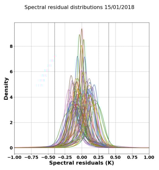
Figure 1.
Density functions (absolute numbers) of spectral residuals in all selected retrieval channels, for 15 January 2018. Each channel is plotted with a different color.
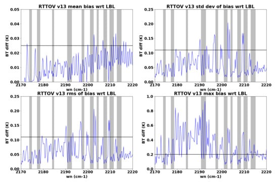
Figure 2.
RTTOV version 13 (with coefficients version 13) bias analysis with respect to line by line calculations with LBLRTM v12.8, for the set of 83 profiles used to train RTTOV, in Brightness Temperature (BT) units: mean bias (with horizontal black line at 0.025 K), standard deviation of the bias (with horizontal black line at 0.11 K), root-mean-square (rms, with horizontal black line at 0.11 K) of the bias and maximum bias (with horizontal black line at 0.2 K), as a function of the wave number (wn). The gray areas show our N2O retrieval spectral windows.
3.4. Summary of Differences with Respect to Pre-Existing IASI N2O Retrieval Algorithms
Our approach in retrieving and validating N2O from IASI is different from MUSICA and SOFRID in a number of aspects.
- Our NOPIR algorithm uses the 3 spectral band as in SOFRID because it is the most sensitive to N2O within the IASI spectral range, but we have very carefully selected a list of micro-windows to avoid interfering gases instead of adding multiple gases in the retrieval; our selection of IASI spectral channels also allows improved sensitivity down to the lower troposphere, with respect to MUSICA.
- We use RTTOV as radiative transfer, as in SOFRID, but we use the latest available version 13.0.
- Our retrieval is based on the Tikhonov regularization [69,70], with a constraint on the profile shape and not on absolute concentrations. This choice allows observing long-term trends without possible bias linked to the a priori used in the retrieval. With an Optimal Estimation [73] retrieval (as in SOFRID) or a Tikhonov constraint mimicking the inverse of a covariance matrix (MUSICA), either the variability has to be set quite high to allow for the long-term increase (e.g., 10% in MUSICA, 5% in SOFRID), or the a priori must include a trend such as to mimic the expected trend, making the retrieved trend possibly dependent on the a priori trend.
- Our NOPIR retrieval is provided and validated on a pixel basis (like MUSICA, but unlike SOFRID that is validated on a monthly basis), and provides a decent quality also at Arctic and Antarctic stations (none of the other retrievals are presented there) and during day and nighttime (SOFRID uses only nighttime IASI data). We validate integrated N2O columns (instead of only the layer with the highest sensitivity) with the available quality controlled data from NDACC and TCCON stations.
- NOPIR retrieved products have about 2 degrees of freedom (DOF) (more than MUSICA, less than SOFRID) except at high latitudes where the DOF is reduced to about 1 (similar for MUSICA, not considered in SOFRID).
4. Results
The N2O retrieval as described in the previous section is undertaken on each available IASI cloud-free scene for which good quality data is available, since 22 February 2011 (the start of the level 1 PCA data). Then, a quality control is undertaken, to ensure selecting only the highest quality retrieval results (described in Section 4.1). This filtered dataset is analyzed in this section, first in terms of its intrinsic properties, then by comparing it to reference ground-based network data.
4.1. Quality Control
We apply five strict selection criteria to our retrieval results, ensuring that only the best results are exploited. The spectral residuals are the differences between the observation and the modeled spectrum after the retrieval.
- Maximum 10 iterations in the retrieval; after that, the retrieval is stopped and considered non-converging;
- The root-mean-square of the spectral residuals (RMSSR) must be below 0.2 K, which is about the IASI noise in our retrieval spectral range;
- Each spectral channel’s residual must be below 0.4 K, which is about twice the IASI noise in our retrieval spectral range;
- At least 0.75 DOF in the retrieval; below this threshold we consider that the sensitivity was too low to trust the result; this occurs very rarely;
- A retrieved Ts between 200 and 350 K; the minimum boundary allows filtering out scenes with undetected clouds and/or aerosols while the maximum boundary rejects unphysical results, occurring very rarely.
The filters on DOF and Ts only extremely rarely remove pixels for which the convergence was reached. The other two criteria, on the total RMSSR and especially that on single spectral residuals, remove a significant amount of results as can be seen in Figure 3 where the line for the final quality control (black) is almost superimposed on the line for the single residual criterion (cyan). The criterion on the single residuals is indeed very strong: no residual, at any wave number, is allowed with more than twice the IASI noise. Globally, only about 40% of the pixels lead to a good N2O retrieval in 2011, while this ratio is up to about 75% since mid 2016, coinciding with the start of the EUMETSAT IASI level 2 version 6.2.2.
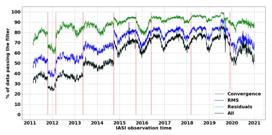
Figure 3.
Statistics on the NOPIR quality control filtering (with previous cloud filtering) as a function of observation date. The cyan curve (filtering on each spectral residual) falls below the black curve (all filters applied). Red vertical lines relate to dates in Table 1, linked to changes in the EUMETSAT IASI operational level 2 processing. A red line has also been added for 16 May 2013, when an update in the EUMETSAT IASI operational level 1 processing occurred [76],which clearly influences the NOPIR retrieval residuals.
The analysis on the quality control of our N2O data also brings interesting information on the evolution of the quality over time. As our retrieval method, N2O a priori and surface emissivity do not change at all over the years (but do vary seasonally), the only possibility for a changed quality over the years is the other input data we use: the IASI level 1c PCA spectra, the IASI level 2 Ts (used as a priori), temperature and humidity profiles (not retrieved) or even the cloud product (used for selecting cloud-free pixels). Indeed, the clear improvements in the number of good quality N2O retrievals are all but one (mid-May 2013) linked to a reported change in the IASI level 2 processor version (see also Table 1). End October 2011, the update (cloud screening) causes a smaller ratio of converging retrievals, which is then corrected at the next update (cloud product) end February 2012. The lower ratio of converging N2O retrievals between these two changes is most probably due to a higher number of unreported cloudy pixels, for which our retrieval is attempted and fails. Mid-May 2013 our ratio of good retrievals is improved, with no change in the EUMETSAT level 2 data processor. However, a calibration change in the IASI level 1c spectra occurred in the processing chain on 16 May 2013 (the IASI point spread function was improved [76]), to which we attribute the improvement in our retrieval residuals. The switch to the IASI level 2 processor version 6 in September 2014 leads to a clear increase in the ratio of converging and of good quality N2O retrievals, attributed mostly to the improved quality in the IASI temperature profiles but also partially to the improved cloud product (improving the convergence ratio). García et al. [17] have also shown that, in the MUSICA algorithm, the EUMETSAT IASI level 2 version 6 IASI data lead to higher quality N2O retrievals than the level 2 version 5 data. The next update in September 2015 shows also some improvements in our ratio of good retrievals, although it is less clear because of the seasonal cycle in that ratio. The next level 2 updates do not seem to have a strong impact on the ratio of good quality results, except for the last one in December 2019, which actually leads to an increase of the spectral residuals in our retrieval.
In addition to the changes in the quality statistics linked to changes in the IASI level 2 processor, there is a seasonal cycle in the ratio of good quality N2O retrievals. This cycle is mostly due to the high latitudes: at high North latitudes there are little good retrievals during the winter and much more during the summer, while at high south latitudes there are few good retrievals all year long. The number of high latitude good retrievals seems to relate to the surface temperature: during the local summer, high north latitudes (especially land areas) heat up more than high south latitudes (see Figure 4, where both the retrieved surface temperature and the number of good retrievals are shown as a monthly mean for June and December 2018), and a higher surface temperature usually leads to a better sensitivity and therefore more good retrievals.
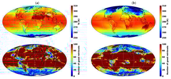
Figure 4.
(Top) Retrieved surface temperature (monthly average) and (bottom) number of good retrievals per grid cell for (a) June and (b) December 2018, using a 1° × 1° lat/lon grid.
After this quality control, there remained areas and periods for which we found the retrieval results doubtful (see for example Figure 5, showing monthly averaged N2O partial columns for June and December 2018): high N2O in the Tropics during Northern Hemisphere spring and summer, high N2O in some high latitude areas during the summer, higher N2O over high altitude mountains as the Andes or plateaus as Tibet.
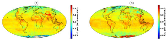
Figure 5.
Retrieved N2O partial column from 800 to 80 hPa (monthly average) for (a) June and (b) December 2018.
The local higher N2O columns in the Tropics, and especially over North Africa and offshore, could be clearly associated with the presence of atmospheric dust aerosols, as seen in Figure 6 where we show the correlation between our retrieved N2O column along the retrieval vertical range and the dust 10 m aerosol optical depth (AOD) from the Mineral Aerosol Profiling from Infrared Radiances (MAPIR) IASI dust retrieval [77], for 1st of June 2018 in the Saharan and dust outflow area (latitude 15 to 35° N, longitude 30° W to 30° E), when a large dust plume was observed in the Western part of the Sahara and offshore. Although there is a non-negligible variability of the retrieved N2O column, it is clear that the latter tends to increase with large dust AOD. This can be linked either to the direct impact of dust aerosols on the radiance, which is broadband, or to the indirect impact of the dust on the EUMETSAT IASI retrieval of temperature and humidity, which then impacts our N2O retrieval. We decided to filter out the “dusty” scenes, using a threshold of maximum MAPIR 10 m dust AOD of 0.25. Obviously, filtering all plausibly “dusty” pixels even with very low AOD would prevent from observing N2O in most of the dust belt during the dust season, so a compromise must be made. Figure 7 shows the result of the additional dust filter for the 1st of June 2018. It is obvious that, in this case, most of the local high N2O values are linked to the presence of dust and are removed when applying the additional filtering. Figure 8 shows what would the N2O overestimation be on a monthly basis for June 2018 if not filtering out dusty pixels. This overestimation can reach 2.5% locally in the monthly average, so it is clearly not negligible. It would not be reflected in most validation exercises, as most instruments do not provide data under heavy dusty conditions (as for cloudy conditions). All data presented from here on are filtered with this additional quality criterion on the dust AOD.

Figure 6.
Correlation between the MAPIR [77] dust AOD and our retrieved N2O partial column along the retrieval vertical range, for the 1st of June 2018 in the Saharan area (latitude 15 to 35° N, longitude 30° W to 30° E).
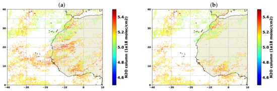
Figure 7.
N2O partial column along the retrieval vertical range for the 1st of June 2018, (a) with the standard quality control and (b) with the added filtering to remove dusty scenes.
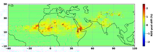
Figure 8.
Monthly average for June 2018 of the difference between the retrieved N2O partial column using simple quality control or with the additional dust filter.
Regarding the high N2O partial column at high latitudes during the summer and over high altitude mountains and plateaus, the problem seems to be linked to a low sensitivity of the retrieval. Indeed, in those areas during the summer (i.e., central Greenland, the Andes and the Tibetan Plateau in June, Antarctica in December) the number of good retrievals and the surface temperature are lower (see also Figure 9, showing the DOF). In addition, at high latitudes there could be a larger bias in the surface emissivity, and a higher propagated temperature profile uncertainty (see Section 4.2). For the high altitude areas, there could be a bias in the retrieval linked to a non-physical a priori profile. Indeed, we use averages by latitude bands, which could not well represent vertical profiles at the high altitude locations.
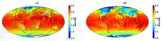
Figure 9.
Monthly mean N2O DOF for (a) June 2018 and (b) December 2018 (after full quality control).
4.2. Characterization of the Retrieved N2O Profiles: Error Analysis, Averaging Kernels and Information Content
The OEM formalism to characterize the retrieval’s sensitivity and perform an error analysis can be used also when the OEM constraint matrix (atmospheric variability) is replaced by a profile shape constraint, as in the Tikhonov regularization scheme. Averaging kernels are calculated during our retrieval, following Rodger’s theory [73]. All data shown have undergone the full quality control.
The trace of the averaging kernel matrix represents the number of degrees of freedom (DOF) for the retrieval. Here, we look separately at the DOF for Ts and N2O retrievals. For Ts, the DOF is always very close to 1 (not shown), meaning that its retrieval should be independent of the a priori, provided that this a priori value is close enough to the true value (the standard deviation was set to 1 K). The N2O DOF is close to 2 in the Tropics area, about 1.5 over mid-latitude oceans, and can lower to 1 at high latitudes (see Figure 9). Of course, over land there are local/seasonal patterns in the sensitivity, linked to the surface emissivity and temperature, which control the total amount of radiance emitted. For example, over mid-latitude land the DOF clearly depends on the season, being higher when the Ts is higher (see Figure 4). We also observe that the DOF is lower over high altitude mountains and plateaus, especially the Tibetan Plateau and the Andes, again correlated with the lower Ts. The high-latitude lands show an interesting pattern of sensitivity, having a higher sensitivity during the winter than during the summer. This is linked to the thermal contrast between the surface and the atmosphere, which is low over land at high latitude during the summer (Ts is close to the atmospheric temperature) while high during the winter (Ts is even lower than 250 K, much lower than the atmosphere, creating a thermal contrast which gives more sensitivity even if it is a negative contrast). Within a IASI swath, one can clearly see (Figure 10a) a higher DOF for higher viewing zenith angle (VZA), as is also seen in Figure 10b. This link between DOF and VZA does, however, not relate to any impact on the N2O column itself. There is no significant difference in DOF for daytime and nighttime (no shown), except when there is a significant difference in Ts.

Figure 10.
(a) N2O DOF for 15 December 2018 during day-time and (b) N2O retrieval DOF as a function of satellite VZA for global data in December 2018. The result is similar for other months.
To characterize the retrieval’s uncertainty, we propagate the spectral noise and uncertainties of the temperature and humidity profiles to the retrieved N2O profiles, using Rodger’s formalism based on Gaussian statistics in particular Equation (3).16 therefrom in Ref. [73]. Doing so requires knowledge of uncertainties of those parameters. The spectral noise is defined, in the retrieval, to the approximate true value. The uncertainty on the IASI level 2 temperature and humidity profiles is set, for this analysis, to 1 K and 10%, respectively. Those were the target accuracy at the design of the instrument [78], and the real accuracy evolves over time with the different algorithm versions, which would be difficult to follow for our error analysis. As the propagated uncertainties are random, the calculated N2O error is also random.
Figure 11 and Figure 12 show examples of the retrieved versus a priori profiles, averaging kernels and error analysis, for a random tropical pixel and a random high latitude pixel. Of course, these vary with the local situation, but general tendencies can be observed. The a priori (GEOS-Chem-based climatology) and retrieved N2O profiles are also shown. One clearly sees that the retrieved profile can deviate a lot from the a priori profile, in terms of absolute values. This is expected because the a priori is an average of GEOS-Chem simulations over the years 2006 to 2016, while we look here at data during 2018, for which a significantly higher N2O concentration is expected. This large absolute variation in the N2O concentration is easily allowed by the Tikhonov regularization scheme that constrains only on the profile shape.
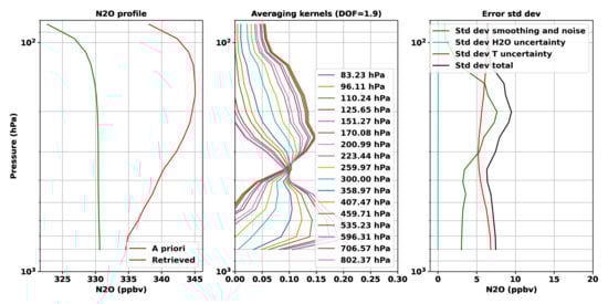
Figure 11.
Example of retrieval results, averaging kernels and error analysis (standard deviation of the covariance matrices) for a tropical latitude (10.6° S 0.1° E), 15 December 2018.
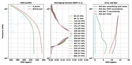
Figure 12.
Example of retrieval results, averaging kernels and error analysis for a high South latitude (80.2° S, 0.2° E), 15 December 2018.
The averaging kernels (rows of the averaging kernel matrix) are broad, as expected with approximately 2 DOF. When the DOF tends to 1, the averaging kernels for all altitudes become identical. Averaging kernels sometimes seem to show a good sensitivity in the lowest layers, however, this originates again in the profile shape constraint and not in the radiance sensitivity to N2O in low layers. Indeed, the N2O Jacobians (see Figure 13 for an example) show a huge decrease in sensitivity when going towards the surface. There is still a significant sensitivity to the lowest retrieval level (the lowest level in the plot), but the sensitivity continues to drop drastically below. This is the reason for not including levels lower than about 800 hPa in the retrieval. Following von Clarmann et al. [79], we verified that the row sum of the averaging kernels (also called measurement response function) are unity, “ensuring that the retrieval is a smoothed but unbiased representation of the true profile” (except for the measurement and parameter error propagation).
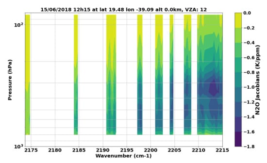
Figure 13.
Example of N2O Jacobians at the NOPIR retrieval wave numbers, for 15 June 2018 at 19.5° N, 39.1° W.
The error analysis can vary much for different situations, but it usually shows similar properties. First, the N2O uncertainty linked to propagating uncertainty on the water vapor content is extremely low, which is consistent with our strategy to avoid all spectral channels impacted (significantly) by interfering gases. Second, the impact of the spectral noise and vertical smoothing (due to the constraint) on the retrieved N2O is significant and usually of the same order of magnitude as the propagated uncertainty on the temperature profile. Third, the total uncertainty (linked to spectral noise, vertical smoothing, uncertainties in water vapor and temperature profiles) is usually between 5 and 10 ppb (1–3%) along the vertical profile. Finally, at high latitudes, the impact of the uncertainty on the temperature profile increases significantly and usually dominates the error analysis. The total uncertainty exceeds 3% in that case. Figure 14 shows, for 15 December 2018, the calculated total uncertainty on the N2O partial columns along the retrieval vertical range. There is a significant difference (of about 0.5%, not shown) between daytime and nighttime uncertainties over surfaces subject to large temperature changes, as deserts, with a higher uncertainty at night when the surface is colder. Indeed, the total uncertainty is correlated to Ts as shown in Figure 15, and this correlation is due to the propagated T profile uncertainty (not shown).

Figure 14.
Example of N2O partial column total uncertainty due to vertical smoothing, spectral noise, water vapor and temperature profiles, for 15 December 2018.
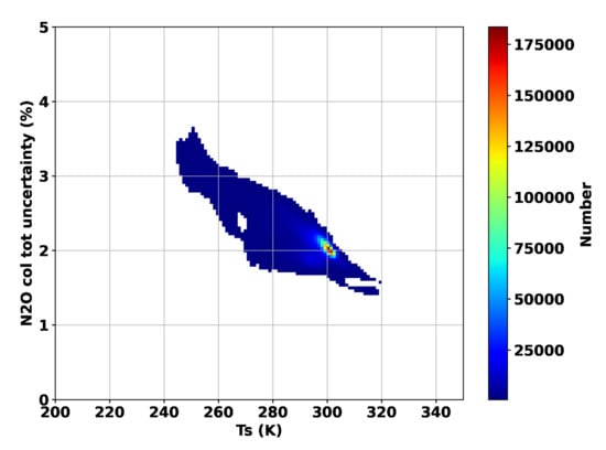
Figure 15.
N2O partial column total uncertainty (due to vertical smoothing, spectral noise, water vapour and temperature profiles) correlation with surface temperature, for 15 December 2018.
There remains one important parameter for which the uncertainty is not propagated in this analysis: the surface emissivity. RTTOV does not produce Jacobians with respect to surface emissivity, therefore the generalized propagation of its uncertainty can not be done. However, we evaluated the impact of a change in surface emissivity on the retrieved N2O by a sensitivity study on a very limited data set (15 June 2018 and 15 December 2018, not shown): a 5% change in the surface emissivity, which is unreasonably high over oceans or well-analyzed land surfaces, but could occur at difficult land surfaces such as deserts, mountains or ice, may lead to a maximum 2.5% change in the retrieved N2O column, the largest impact observed at night over land (lower Ts).
Finally, the uncertainty on RTTOV model spectra in the retrieval windows was discussed in Section 3.3: the estimated RTTOV mean bias is a factor of magnitude lower than the IASI noise and is therefore not considered relevant. The RTTOV bias, however, does not contain the uncertainty linked to the spectroscopy; that uncertainty is accounted for in the use of an inflated noise for the retrieval.
The total uncertainty, being 1–3% over ocean, possibly up to about 5% at high latitudes and/or over surface with high uncertainty in the emissivity (as deserts or ice) is high with respect to the low variability of N2O, but still in the same range as the ground-based observation uncertainties.
4.3. Validation against NDACC and TCCON
4.3.1. Comparison Methodology
The methodology for the validation of the IASI N2O data against NDACC and TCCON data is very similar, with small differences linked to the fact that NDACC provides vertical profiles of N2O vmr while TCCON provides dry-air column-averaged mole fractions. We first describe in detail the method for NDACC comparisons, then we will highlight the differences for the TCCON comparisons. Co-locations are done between IASI and NDACC observations, with maximum 100 km distance and 6 h time difference. This maximum time difference is long, but necessary because the NDACC observations are done only a few times per day. This should, however, not be a problem because the N2O amount does not have a pronounced diurnal cycle. The allowed distance between IASI and the ground-based instrument has to be considered in comparison to the IASI pixel size (reminder: 12 km circle at nadir, 39 by 20 km ellipse at scan edges). The selected 100 km allows having enough co-located IASI measurements to reduce the variability in the comparisons. For the same reason, for each NDACC observation, the co-located IASI pixels are averaged. If a ground-based observation is co-located with less than 5 IASI pixels, it is not considered in the validation. In the case more than 10 pixels match the co-location criteria, only the 10 closest in time are taken into account. As TCCON observations are much more frequent along a day, the maximum time difference allowed for those comparisons is reduced to 30 min. For both networks, after co-location with satellite observations, the ground-based data are filtered for outliers as follows: (1) we average the ground-based data (as dry-air column-averaged mole fractions, the standard TCCON unit and applying a conversion for NDACC data originally in vmr units) with a binomial rolling window of size 5 on bi-daily temporal median values (so, the rolling window spans over 10 days); (2) an observation is removed if its difference with the rolling mean exceeds 1.5 the interquartile range (IQR, the difference between the 75th and 25th percentiles) away from the quartiles.
The inter-comparisons are undertaken based on the theory from Rodgers and Connor [80]. The retrieved N2O profiles are adjusted to take into account the difference in a priori profiles for the ground-based (NDACC or TCCON) and IASI retrievals. The ground-based a priori profiles are used as common profiles. This choice avoids grid mismatch issues when re-gridding because the satellite grid has a limited vertical range. The ground-based a priori is re-gridded to the IASI vertical grid using linear interpolation. In case the ground-based vertical grid was set up at a higher surface altitude than the bottom of the satellite profile (at high altitude stations), it is continued downwards by linear extrapolation. Because the ground-based a priori is the common profile, only the IASI retrieved profiles are adjusted as in Rodgers and Connor [80]:
where x represents the retrieved profile, A is the averaging kernel, I is the identity matrix of the same size as A and stands for “adjusted”, for “a priori”, and for “regridded”. In a second step, which further reduces the impact of the common a priori in the comparison, the NDACC retrieved profiles (regridded on the IASI vertical grid) are smoothed using the IASI averaging kernels:
where stands for “smoothed”. Then, both profiles are integrated in a partial column along the IASI retrieval range (800 to 80 hPa). The IASI bias discussed in the next section is:
where stands for “partial column”.
For TCCON observations, only a total column value is retrieved, and the comparison methodology therefore has to be slightly adapted. A pseudo-retrieved TCCON profile is obtained from the TCCON a priori profile, multiplied by a scaling factor being the ratio between the retrieved TCCON column and the a priori TCCON column:
where and are, respectively, the TCCON a priori and retrieved dry-air column-averaged mole fractions. An additional difference is that NDACC products are N2O vertical profiles of vmr, while the pseudo retrieved TCCON profiles () are in dry-air partial column mole fractions. Therefore, the IASI profiles have to be converted to the same units, using the dry-air partial columns from the satellite data.
4.3.2. Analysis
Different ways to look at the data will be used:
- Full period bias analysis at selected stations (the analysis was done at all stations, but it is impossible to show all plots): to determine if the data quality changes over time;
- Weekly bias analysis at all stations over a short period: to analyze any seasonal patterns in the bias;
- Bias and standard deviation for all stations for the period of improved quality: for an assessment of the NOPIR accuracy and precision;
- Correlation between ground-based and satellite data.
Long-term bias analyses (see Figure 16, Figure 17 and Figure 18) show a small positive mean bias (less than 4%) of the NOPIR N2O columns. The impact on our data quality of the EUMETSAT IASI level 2 processor upgrade to version 6 in September 2014 is obvious. The IASI retrieved N2O variability (within the quality controlled data) is much higher before that date, at all stations. At some stations (but not all) there is also a positive step in the bias at that date. This inconsistency in the time series and the larger variability in the older data led to the decision to use only our N2O retrieved data starting on 30 September 2014 (when the EUMETSAT IASI level 2 processor version 6 was switched on). This also explains why we have not considered processing the IASI retrievals prior to 2011 when the PCA do not exist: it would represent a significant development time to use the “non-PCA” IASI data and would not bring very interesting results. The further updates in the IASI level 2 data version lead to smaller differences in the N2O retrievals, not very clearly visible in Figure 17 and Figure 18 (except maybe a lower bias at Wollongong with the IASI level 2 version 6.1.1 from end 2015 to mid 2016), but clearly visible if one creates time series on large geographical averages, to reduce the variability (not shown).

Figure 16.
Validation time series at the NDACC Lauder station: time series of (top) relative bias of the averaged co-located IASI data and (bottom) IASI adjusted N2O partial columns () and ground-based (GB) smoothed partial columns (). Statistics of the comparisons are also shown: mean and median bias, standard deviation of the bias and median of absolute deviations (MAD) adjusted to correspond to the standard deviation of a Gaussian distribution (multiplied by 1.4826). Dotted red vertical lines represent the changes in the EUMETSAT IASI level 2 processor version listed in Table 1, and in addition the 16 May 2013 when an update in the EUMETSAT operational level1 processing occurred [76].
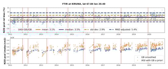
Figure 17.
Same as Figure 16 for the NDACC Kiruna station.
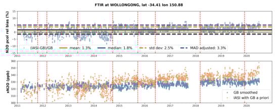
Figure 18.
Same as Figure 16 for the TCCON Wollongong station but here in terms of dry-air column-averaged mole fractions, the standard TCCON unit.
Figure 19 shows the weekly averaged relative bias at NDACC and TCCON stations, for the years 2017 and 2018. Except for some very limited periods and stations, the IASI bias is positive. It remains mostly below 5%, with no clear seasonal pattern. The IASI retrievals at high latitudes overall present a slightly larger bias, confirming what was already identified in the analysis of the N2O partial columns (Section 4.1). Comparisons at NDACC stations are significantly different for years 2017 and 2018 (with a higher IASI bias in 2018), while at TCCON stations the bias is very similar for both years. This is yet unexplained.
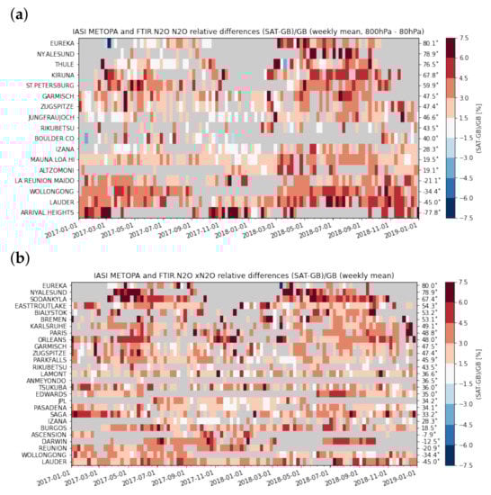
Figure 19.
Relative bias of IASI NOPIR N2O at (a) NDACC and (b) TCCON stations: weekly average for the years 2017 and 2018.
Figure 20 shows the mean bias and the bias standard deviation for all NDACC and TCCON stations for the period since 30 September 2014 until end 2020. As comparison (not shown), the validation was also undertaken without the a priori substitution and averaging kernel smoothing, and leads to very similar results (overall bias differences within 0.2%, standard deviation differences within 0.3%). It is also interesting to note that the N2O spectroscopy should not be responsible for the difference between the ground-based and IASI N2O data, because the N2O spectroscopy has not changed between HITRAN2008 (used in the ground-based retrievals) and HITRAN2012 (used to create the RTTOV coefficient tables) [81].
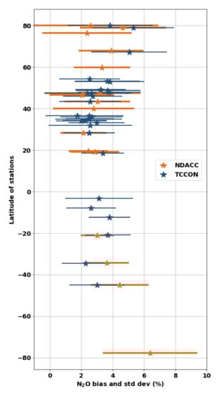
Figure 20.
Mean relative bias and standard deviations (std dev) of IASI NOPIR N2O at NDACC and TCCON stations, for comparisons from 30 September 2014 to 31 December 2020.
Except at high latitude stations, the (positive) bias is between 1.8 and 4%. In Antarctica (Arrival Heights), the IASI bias with respect to NDACC is as high as 6.4%, yet unexplained except by plausible difficulties (lower sensitivity and larger uncertainties) for both ground-based and IASI retrievals in this difficult location. At high North latitude stations, the bias with respect to TCCON is significantly larger than the usual bias while the bias with respect to NDACC remains below 4%, except at Ny Ålesund. For the latter station, we attribute the larger IASI bias to a low bias of the NDACC data, for which indeed the systematic and random uncertainties are reported to be, respectively, about 4% and 2%, much higher than at most stations. The difference between NDACC and TCCON comparisons at high north latitudes can be linked to the work of Zhou et al. [82], who compared total column averaged N2O from NDACC and TCCON at 7 stations (Ny Ålesund, Sodankylä, Bremen, Izaña, Réunion, Wollongong and Lauder). They showed that at high north latitudes, NDACC columns tend to be larger than TCCON columns (especially when the station is inside the polar vortex: TCCON tends to underestimate the N2O column), which could explain that in our comparisons the IASI bias, being positive, is much larger with respect to TCCON than NDACC, at all northern latitude stations.
On the other hand, at Wollongong and Lauder the TCCON columns are reported by Zhou et al. [82] to be much larger than the NDACC columns, explaining that our IASI positive bias is larger with respect to NDACC than TCCON at those stations.
The standard deviation of the comparisons varies between 1.5 and 3%, exceeding the expected natural seasonal and latitudinal variability (respectively, of 1 ppb/0.3% and 2 ppb/0.6%). The standard deviation of the comparisons is, however, in the range of the random uncertainty on the IASI retrievals, and also showing larger values at higher latitudes where the uncertainty is larger.
Finally, the Pearson correlation between IASI and NDACC/TCCON N2O data is of, respectively, 0.44 and 0.49 if grouping all data from a network (all stations, all years) in a single analysis. However, we think that the correlation is not very representative when characterizing the data quality of a parameter with very little variability as is N2O (1 ppb seasonal variability, 2 ppb latitudinal variability, 5.7 ppb along 6 years, for a total of about only about 2.6% expected variability over the whole analysis, well below the combined uncertainties of the compared data).
5. Discussion
We have presented a new N2O retrieval from IASI, with the Nitrous Oxide Profiling from Infrared Radiances (NOPIR) algorithm. We provided a description of the technical setup of the retrieval, of its quality control, its sensitivity and uncertainties and its validation against ground-based data from NDACC and TCCON networks. The N2O integrated columns obtained with the NOPIR algorithm are overall of very good quality: the validation at the pixel level shows overall a 1.8 to 4% positive bias (with 1.5 to 3% standard deviation) of NOPIR columns with respect to ground-based observations, except at high North latitude TCCON stations (where another analysis has shown that TCCON data can be biased [82]), and in Antarctica (yet unexplained, but there is only one NDACC station available and its data is reported with a relatively high mean systematic bias of 3.5%).
The estimated uncertainties on the NOPIR columns are usually of 1 to 3% (mostly random, but there is certainly a systematic component: the updates in the IASI level 2 data from EUMETSAT lead to step increases in the NOPIR retrieved N2O), linked mostly to the IASI spectral noise, the vertical smoothing due to the retrieval’s constraint and uncertainties in the temperature profile. At high latitudes, the uncertainty linked to the temperature profiles increases. The surface emissivity introduces a significant additional uncertainty (possibly up to 2.5% of unknown sign and varying with the season) over land where the emissivity is difficult to characterize, such as snow or deserts. The ground-based NDACC data also bears a systematic uncertainty of 2 to 4.4% of unknown sign, and random of 0.5 to 2% (as reported in the data files). The TCCON columns bear no systematic uncertainty (corrected in the processing) and a mean estimated random uncertainty of maximum about 0.5% (except at Ascension where it goes up to 0.9%, see Table 3) to which about 1% should be added as uncertainty in the systematic bias correction during the TCCON processing [10]. The IASI bias with respect to ground-based observations falls within the sum of the uncertainties on the compared values.
One can argue that uncertainties such as those of NOPIR, NDACC or TCCON are too high with respect to the expected very low natural variability of N2O, currently reported to be of about 1 ppb (0.3%) seasonally or 2 ppb (0.6%) geographically [3]. However, the local emissions lead to an increased local N2O column, and that might well exceed the observation uncertainties. This analysis is beyond the scope of the current manuscript, but is certainly an interesting future prospect. With the properties of the IASI instrument, we are not convinced that the quality of the N2O column can be improved enough to reach N2O source detection with sufficient confidence. However, the future instrument IASI-NG (New Generation) that will fly onboard the Metop-SG (Second Generation) series of platforms (the first is planned for launch in 2024) will have a twice better signal-to-noise ratio, and a twice higher spectral resolution. We expect that will allow obtaining an improved N2O product, with higher sensitivity (increased DOF) and lower uncertainty, which might allow source detection.
The analysis of long-term trends in the N2O abundance is already possible with the current IASI instrument, as was shown by Barret et al. [18]. Our product, however, suffers from the inconsistencies in the EUMETSAT IASI level 2 temperature (and humidity) vertical profiles, used to set up the atmosphere in NOPIR. We have discussed the significant impact of the update of the EUMETSAT IASI level 2 processor from version 5 to version 6, leading to the decision to use only data from the version 6 starting in September 2014. A short-term trend analysis was attempted using 6 years of data (2015 to 2020), but we rejected that analysis because it was very clear that even the small changes in the EUMETSAT IASI level 2 processing version (listed in Table 1) lead to small jumps in our N2O column time series. Those jumps are of the order of +/− 0.5 to 1% at most, observed only after significant spatial averaging of the data to remove the noise (in the attempt to observe trends, e.g., a 30° latitude band) while barely seen in the validation. Those jumps, occurring four times in 6 years, are clearly enough to prevent the successful observation of a trend expected to be about 0.3%/year. Our algorithm development in this work was aimed at a possible operational retrieval, therefore using the best data available if the retrieval is run in near-real-time: that is indeed the IASI level 2 data, available timely and aiming at the best possible quality in near-real-time. In that sense, our development can be considered very successful and the NOPIR product is of very good quality. To observe trends, the long-term consistency is the most important factor, beyond any recurring bias that can be corrected for. In a future work, we will adapt NOPIR for a trend analysis specific version using a consistent data set of temperature and humidity profiles, such as the European Center for Medium-range Weather Forecasts (ECMWF) reanalysis data.
Author Contributions
Conceptualization, S.V. and M.D.M.; data curation, S.V., B.L., C.V., M.B., N.M.D., D.G.F., O.G., J.W.H., F.H., R.K., N.K., M.M., D.B.M., I.M., T.N., J.N., H.O., I.O., C.P., M.R., M.S., C.P.S., M.K.S., K.S. (Kei Shiomi), D.S., K.S. (Kimberly Strong), R.S., Y.T., V.A.V., M.V., T.W., K.C.W., D.W., M.Z. and M.D.M.; formal analysis, S.V. and B.L.; funding acquisition, S.V. and M.D.M.; investigation, S.V. and B.L.; methodology, S.V., B.L. and C.V.; project administration, S.V. and M.D.M.; resources, S.V., B.L., C.V., M.B., N.M.D., D.G.F., O.G., J.W.H., F.H., R.K., N.K., M.M., D.B.M., I.M., T.N., J.N., H.O., I.O., C.P., M.R., M.S., C.P.S., M.K.S., K.S. (Kei Shiomi), D.S., K.S. (Kimberly Strong), R.S., Y.T., V.A.V., M.V., T.W., K.C.W., D.W., M.Z. and M.D.M.; software, S.V., B.L., C.V., M.B., N.M.D., D.G.F., O.G., J.W.H., F.H., R.K., N.K., M.M., D.B.M., I.M., T.N., J.N., H.O., I.O., C.P., M.R., M.S., C.P.S., M.K.S., K.S. (Kei Shiomi), D.S., K.S. (Kimberly Strong), R.S., Y.T., V.A.V., M.V., T.W., K.C.W., D.W., M.Z. and M.D.M.; supervision, S.V. and M.D.M.; validation, S.V. and B.L.; visualization, S.V. and B.L.; writing—original draft, S.V.; writing—review and editing, S.V., B.L., C.V., M.B., N.M.D., D.G.F., O.G., J.W.H., F.H., R.K., N.K., M.M., D.B.M., I.M., T.N., J.N., H.O., I.O., C.P., M.R., M.S., C.P.S., M.K.S., K.S. (Kei Shiomi), D.S., K.S. (Kimberly Strong), R.S., Y.T., V.A.V., M.V., T.W., K.C.W., D.W., M.Z. and M.D.M. All authors have read and agreed to the published version of the manuscript.
Funding
This research and the APC were funded by the Belgian Science Policy (belspo)/European Space Agency (ESA) PROgramme for the Development of scientific EXperiments (PRODEX) Hyperspectral atmospheric IR Sounding mission (HIRS) project, grant number 400013459. K.C.W. and D.B.M. acknowledge support from the US National Oceanic and Atmospheric Administration (grant no. NA13OAR4310086). The Ascension Island TCCON station has been supported by the European Space Agency (ESA) under grant 4000120088/17/I-EF and by the German Bundesministerium für Wirtschaft und Energie (BMWi) under grants 50EE1711C and 50EE1711E. We thank the ESA Ariane Tracking Station at North East Bay, Ascension Island, for hosting and local support. The NDACC site at Rikubetsu is operated as parts of the joint research programme of the Institute for Space-Earth Environmental Research (ISEE), Nagoya University, and supported in part by the GOSAT series project. TCCON sites at Tsukuba, Rikubetsu and Burgos are supported in part by the GOSAT series project. Burgos is supported in part by the Energy Development Corp. Philippines. Measurements at Lauder and Arrival Heights are core funded by NIWA through New Zealand’s Ministry of Business, Innovation and Employment Strategic Science Investment Fund. D.S. thanks Antarctica New Zealand for providing support for the measurements at Arrival Heights. The Paris TCCON site has received funding from Sorbonne Université, the French research center CNRS, the French space agency CNES, and Région Île-de-France. The University of Liège (ULiège) team has been primarily supported by the Fonds de la Recherche Scientifique (F.R.S.—FNRS, Brussels, Belgium), the Federation Wallonie-Bruxelles (FWB, Belgium) and by the GAW-CH program of MeteoSwiss (Zürich, Switzerland). C.S. thanks the International Foundation High Altitude Research Stations Jungfraujoch and Gornergrat (HFSJG, Bern) for supporting the facilities needed to perform the FTIR observations at Jungfraujoch. The TCCON and NDACC sites at Réunion Island is operated by the Royal Belgian Institute for Space Aeronomy and local activities supported by LACy/UMR8105 and by OSU-R/UMS3365—Université de La Réunion. The TCCON Réunion Island site is financially supported since 2014 by the EU project ICOS-Inwire and the ministerial decree for ICOS (FR/35/IC1 to FR/35/IC6). The National Center for Atmospheric Research is sponsored by the National Science Foundation. The NCAR FTS observation programs at Thule, GR, Boulder, CO and Mauna Loa, HI are supported under contract by the National Aeronautics and Space Administration (NASA). The Thule work is also supported by the NSF Office of Polar Programs (OPP). We wish to thank the Danish Meteorological Institute for support at the Thule site and NOAA for support at the MLO site. The TCCON Nicosia site has received additional support from the European Union’s Horizon 2020 research and innovation programme under grant agreement No. 856612 (EMME-CARE) and the Cyprus Government, and by the University of Bremen. The Eureka TCCON and NDACC measurements were made at the Polar Environment Atmospheric Research Laboratory by the Canadian Network for the Detection of Atmospheric Change, primarily supported by the Natural Sciences and Engineering Research Council of Canada, Environment and Climate Change Canada, and the Canadian Space Agency. The Izaña NDACC and TCCON station has been supported by the German Bundesministerium für Wirtschaft und Energie (BMWi) via DLRunder grants 50EE1711A and by the Helmholtz Association via the research programme ATMO, and by AEMet. NMD is supported by an Australian Research Council (ARC) Future Fellowship, FT180100327. The Darwin and Wollongong TCCON/NDACC sites have been supported by a series of ARC grants, including DP160100598, DP140100552, DP110103118, DP0879468 and LE0668470, and NASA grants NAG5-12247 and NNG05-GD07G.
Data Availability Statement
The data is being prepared to be available on iasi.aeronomie.be and with a DOI.
Acknowledgments
The IASI data used in this publication was obtained from the EUMETSAT, and is freely available. The ground-based data used in this publication were obtained as part of the Network for the Detection of Atmospheric Composition Change (NDACC) and the Total Carbon Column Observing Network (TCCON). The NDACC data is available through the website www.ndacc.org. The TCCON data were obtained from the TCCON Data Archive hosted by CaltechDATA available online (accessed on 21 January 2022): https://tccondata.org. The IT service at BIRA-IASB is acknowledged for support in the processing of the data.
Conflicts of Interest
The authors declare no conflict of interest. The funders had no role in the design of the study; in the collection, analyses, or interpretation of data; in the writing of the manuscript, or in the decision to publish the results.
Abbreviations
The following abbreviations are used in this manuscript:
| ACE-FTS | Atmospheric Chemistry Experiment Fourier Transform Spectrometer |
| AIRS | Atmospheric Infrared Sounder |
| AGAGE | Advanced Global Atmospheric Gases Experiment |
| AMSU | Advanced Microwave Sounding Unit |
| BT | Brightness Temperature |
| DOF | Degrees of Freedom |
| EUMETSAT | European Organisation for the Exploitation of Meteorological Satellites |
| FTIR | Fourier-Transform InfraRed |
| GB | Ground-based |
| GEOS | Goddard Earth Observing System |
| GGGRN | Global Greenhouse Gas Reference Network |
| HITRAN | HIgh-resolution TRANsmission molecular absorption |
| IASI | Infrared Atmospheric Sounding Interferometer |
| IASI-NG | Infrared Atmospheric Sounding Interferometer New-Generation |
| IPSF | Instrument Point Spread Function |
| IRWG | InfraRed Working Group |
| LBLRTM | Line-By-Line Radiative Transfer Model |
| LEO | Low Earth Orbit |
| MAPIR | Mineral Aerosol Profiling from Infrared Radiances |
| MERRA | Modern-Era Retrospective Analysis for Research and Applications |
| MIPAS | Michelson Interferometer for Passive Atmospheric Sounding |
| MHS | Microwave Humidity Sounder |
| MLS | Microwave Limb Sounder |
| MUSICA | MUlti-platform remote Sensing of Isotopologues for investigating the Cycle of |
| Atmospheric water | |
| NASA | National Aeronautics and Space Administration |
| NDACC | Network for the Detection of Atmospheric Composition Change |
| NOAA | National Oceanic and Atmospheric Administration |
| NOPIR | Nitrous Oxide Profiling from Infrared Radiances |
| OEM | Optimal Estimation Method |
| PCA | Principal Components Analysis |
| PWLR | Piece-Wise Linear Regression |
| RMSSR | Root Mean Square of Spectral Residuals |
| RTTOV | Radiative Transfer for TOVS |
| SOFRID | SOftware for a Fast Retrieval of IASI Data |
| TCCON | Total Carbon Column Observing Network |
| TES | Tropospheric Emission Spectrometer |
| TIR | Thermal InfraRed |
| WN | Wavenumber |
References
- Canadell, J.G.; Monteiro, P.M.; Costa, M.H.; da Cunha, L.C.; Cox, P.M.; Eliseev, A.V.; Henson, S.; Ishii, M.; Jaccard, S.; Koven, C.; et al. Global Carbon and other Biogeochemical Cycles and Feedbacks. In Climate Change 2021: The Physical Science Basis. Contribution of Working Group I to the Sixth Assessment Report of the Intergovernmental Panel on Climate Change; Cambridge University Press: Cambridge, UK, 2021; in press. [Google Scholar]
- Prather, M.J.; Hsu, J.; DeLuca, N.M.; Jackman, C.H.; Oman, L.D.; Douglass, A.R.; Fleming, E.L.; Strahan, S.E.; Steenrod, S.D.; Søvde, O.A.; et al. Measuring and modeling the lifetime of nitrous oxide including its variability. J. Geophys. Res. Atmos. 2015, 120, 5693–5705. [Google Scholar] [CrossRef] [PubMed]
- Stocker, T.; Qin, D.; Plattner, G.K.; Tignor, M.; Allen, S.; Boschung, J.; Nauels, A.; Xia, Y.; Bex, V.; Midgley, P. (Eds.) IPCC, 2013: Climate Change 2013: The Physical Science Basis. Contribution of Working Group I to the Fifth Assessment Report of the Intergovernmental Panel on Climate Change; Cambridge University Press: New York, NY, USA, 2013. [Google Scholar]
- Tian, H.; Xu, R.; Canadell, J.G.; Thompson, R.L.; Winiwarter, W.; Suntharalingam, P.; Davidson, E.A.; Ciais, P.; Jackson, R.B.; Janssens-Maenhout, G.; et al. A comprehensive quantification of global nitrous oxide sources and sinks. Nature 2020, 586, 248–256. [Google Scholar] [CrossRef] [PubMed]
- Ravishankara, A.R.; Daniel, J.S.; Portmann, R.W. Nitrous Oxide (N20): The Dominant Ozone-Depleting Substance Emitted in the 21st Century. Science 2009, 326, 123–125. [Google Scholar] [CrossRef] [Green Version]
- AGAGE Internet Site. Available online: https://agage.mit.edu/ (accessed on 3 August 2021).
- Prinn, R.G.; Weiss, R.F.; Arduini, J.; Arnold, T.; DeWitt, H.L.; Fraser, P.J.; Ganesan, A.L.; Gasore, J.; Harth, C.M.; Hermansen, O.; et al. History of chemically and radiatively important atmospheric gases from the Advanced Global Atmospheric Gases Experiment (AGAGE). Earth Syst. Sci. Data 2018, 10, 985–1018. [Google Scholar] [CrossRef] [Green Version]
- NOAA Global Greenhouse Gas Reference Network Internet Site. Available online: https://gml.noaa.gov/ccgg/about.html (accessed on 8 September 2021).
- TCCON Internet Site. Available online: http://www.tccon.caltech.edu/ (accessed on 3 August 2021).
- Wunch, D.; Toon, G.C.; Sherlock, V.; Deutscher, N.M.; Liu, X.; Feist, D.G.; Wennberg, P.O. The Total Carbon Column Observing Network’s GGG2014 Data Version. Tech. Rep. 2015. Available online: https://doi.org/10.14291/tccon.ggg2014.documentation.R0/1221662 (accessed on 10 February 2022). [CrossRef]
- NDACC IRWG Internet Site. Available online: https://www2.acom.ucar.edu/irwg (accessed on 3 August 2021).
- Plieninger, J.; von Clarmann, T.; Stiller, G.P.; Grabowski, U.; Glatthor, N.; Kellmann, S.; Linden, A.; Haenel, F.; Kiefer, M.; Höpfner, M.; et al. Methane and nitrous oxide retrievals from MIPAS-ENVISAT. Atmos. Meas. Tech. 2015, 8, 4657–4670. [Google Scholar] [CrossRef] [Green Version]
- Bernath, P.; Steffen, J.; Crouse, J.; Boone, C. Sixteen-year trends in atmospheric trace gases from orbit. J. Quant. Spectrosc. Radiat. Transf. 2020, 253, 107178. [Google Scholar] [CrossRef]
- Livesey, N.J.; Read, W.G.; Froidevaux, L.; Lambert, A.; Santee, M.L.; Schwartz, M.J.; Millán, L.F.; Jarnot, R.F.; Wagner, P.A.; Hurst, D.F.; et al. Investigation and amelioration of long-term instrumental drifts in water vapor and nitrous oxide measurements from the Aura Microwave Limb Sounder (MLS) and their implications for studies of variability and trends. Atmos. Chem. Phys. 2021, 21, 15409–15430. [Google Scholar] [CrossRef]
- Worden, J.; Kulawik, S.; Frankenberg, C.; Payne, V.; Bowman, K.; Cady-Peirara, K.; Wecht, K.; Lee, J.E.; Noone, D. Profiles of CH4, HDO, H2O, and N2O with improved lower tropospheric vertical resolution from Aura TES radiances. Atmos. Meas. Tech. 2012, 5, 397–411. [Google Scholar] [CrossRef] [Green Version]
- Xiong, X.; Maddy, E.S.; Barnet, C.; Gambacorta, A.; Patra, P.K.; Sun, F.; Goldberg, M. Retrieval of nitrous oxide from Atmospheric Infrared Sounder: Characterization and validation. J. Geophys. Res. Atmos. 2014, 119, 9107–9122. [Google Scholar] [CrossRef]
- García, O.E.; Schneider, M.; Ertl, B.; Sepúlveda, E.; Borger, C.; Diekmann, C.; Wiegele, A.; Hase, F.; Barthlott, S.; Blumenstock, T.; et al. The MUSICA IASI CH4 and N2O products and their comparison to HIPPO, GAW and NDACC FTIR references. Atmos. Meas. Tech. 2018, 11, 4171–4215. [Google Scholar] [CrossRef] [Green Version]
- Barret, B.; Gouzenes, Y.; Le Flochmoen, E.; Ferrant, S. Retrieval of Metop-A/IASI N2O Profiles and Validation with NDACC FTIR Data. Atmosphere 2021, 12, 219. [Google Scholar] [CrossRef]
- EUMETSAT. IASI Level 2 Product Guide. Technical Report EUM/OPS-EPS/MAN/04/0033. 2017. Available online: https://www-cdn.eumetsat.int (accessed on 21 January 2022).
- Wiegele, A.; Schneider, M.; Hase, F.; Barthlott, S.; García, O.E.; Sepúlveda, E.; González, Y.; Blumenstock, T.; Raffalski, U.; Gisi, M.; et al. The MUSICA MetOp/IASI H2O and δD Products: Characterisation and long-term comparison to NDACC/FTIR data. Atmos. Meas. Tech. 2014, 7, 2719–2732. [Google Scholar] [CrossRef] [Green Version]
- Schneider, M.; Ertl, B.; Diekmann, C.J.; Khosrawi, F.; Weber, A.; Hase, F.; Höpfner, M.; García, O.E.; Sepúlveda, E.; Kinnison, D. Design and description of the MUSICA IASI full retrieval product. Earth Syst. Sci. Data Discuss. 2021, 2021, 1–51. [Google Scholar] [CrossRef]
- Saunders, R.; Hocking, J.; Turner, E.; Rayer, P.; Rundle, D.; Brunel, P.; Vidot, J.; Roquet, P.; Matricardi, M.; Geer, A.; et al. An update on the RTTOV fast radiative transfer model (currently at version 12). Geosci. Model Dev. 2018, 11, 2717–2737. [Google Scholar] [CrossRef] [Green Version]
- Clerbaux, C.; Boynard, A.; Clarisse, L.; George, M.; Hadji-Lazaro, J.; Herbin, H.; Hurtmans, D.; Pommier, M.; Razavi, A.; Turquety, S.; et al. Monitoring of atmospheric composition using the thermal infrared IASI/MetOp sounder. Atmos. Chem. Phys. 2009, 9, 6041–6054. [Google Scholar] [CrossRef] [Green Version]
- EUMETSAT. EUMETSAT User Notification Service. Available online: https://uns.eumetsat.int/ (accessed on 30 June 2021).
- GEOS-Chem Community. GEOSChem Internet Site. Available online: http://www.geos-chem.org (accessed on 2 August 2021).
- Wells, K.C.; Millet, D.B.; Bousserez, N.; Henze, D.K.; Chaliyakunnel, S.; Griffis, T.J.; Luan, Y.; Dlugokencky, E.J.; Prinn, R.G.; O’Doherty, S.; et al. Simulation of atmospheric N2O with GEOS-Chem and its adjoint: Evaluation of observational constraints. Geosci. Model Dev. 2015, 8, 3179–3198. [Google Scholar] [CrossRef] [Green Version]
- Gelaro, R.; McCarty, W.; Suárez, M.J.; Todling, R.; Molod, A.; Takacs, L.; Randles, C.A.; Darmenov, A.; Bosilovich, M.G.; Reichle, R.; et al. The Modern-Era Retrospective Analysis for Research and Applications, Version 2 (MERRA-2). J. Clim. 2017, 30, 5419–5454. [Google Scholar] [CrossRef]
- NWPSAF. RTTOV Website. Available online: https://nwp-saf.eumetsat.int/site/software/rttov/ (accessed on 23 June 2021).
- Saunders, R.; Hocking, J.; Turner, E.; Havemann, S.; Geer, A.; Lupu, C.; Vidot, J.; Chambon, P.; Köpken-Watts, C.; Scheck, L.; et al. RTTOV-13 Science and Validation Report. Tech. Rep. 2020. Available online: https://nwp-saf.eumetsat.int/site/ (accessed on 10 February 2022).
- Line-By-Line Radiative Transfer Model Internet Site. Available online: http://rtweb.aer.com/lblrtm.html (accessed on 21 January 2022).
- Pougatchev, N.S.; Connor, B.J.; Rinsland, C.P. Infrared measurements of the ozone vertical distribution above Kitt Peak. J. Geophys. Res. Atmos. 1995, 100, 16689–16697. [Google Scholar] [CrossRef] [Green Version]
- Hase, F.; Hannigan, J.; Coffey, M.; Goldman, A.; Höpfner, M.; Jones, N.; Rinsland, C.; Wood, S. Intercomparison of retrieval codes used for the analysis of high-resolution, ground-based FTIR measurements. J. Quant. Spectrosc. Radiat. Transf. 2004, 87, 25–52. [Google Scholar] [CrossRef]
- García, O.E.; Sepúlveda, E.; Schneider, M.; Hase, F.; August, T.; Blumenstock, T.; Kühl, S.; Munro, R.; Gómez-Peláez, A.J.; Hultberg, T.; et al. Consistency and quality assessment of the Metop-A/IASI and Metop-B/IASI operational trace gas products (O3, CO, N2O, CH4, and CO2) in the subtropical North Atlantic. Atmos. Meas. Tech. 2016, 9, 2315–2333. [Google Scholar] [CrossRef] [Green Version]
- TCCON. TCCON Wiki. Available online: https://tccon-wiki.caltech.edu/Main/TCCONSites (accessed on 2 August 2021).
- Strong, K.; Roche, S.; Franklin, J.E.; Mendonca, J.; Lutsch, E.; Weaver, D.; Fogal, P.F.; Drummond, J.R.; Batchelor, R.; Lindenmaier, R. TCCON Data from Eureka (CA), Release GGG2014R3. TCCON Data Archive, Hosted by CaltechDATA. 2019. Available online: https://data.caltech.edu/records/1171 (accessed on 10 February 2022).
- Notholt, J.; Warneke, T.; Petri, C.; Deutscher, N.M.; Weinzierl, C.; Palm, M.; Buschmann, M. TCCON Data from Ny ÅLesund, Spitsbergen (NO), Release GGG2014.R1. TCCON Data Archive, Hosted by CaltechDATA. 2019. Available online: https://data.caltech.edu/records/1289 (accessed on 10 February 2022).
- Kivi, R.; Heikkinen, P.; Kyrö, E. TCCON Data from Sodankyla (FI), Release GGG2014R1. TCCON Data Archive, Hosted by CaltechDATA. 2017. Available online: https://data.caltech.edu/records/20021 (accessed on 10 February 2022).
- Wunch, D.; Mendonca, J.; Colebatch, O.; Allen, N.; Blavier, J.F.L.; Roche, S.; Hedelius, J.K.; Neufeld, G.; Springett, S.; Worthy, D.E.J.; et al. TCCON Data from East Trout Lake (CA), Release GGG2014R1. TCCON Data Archive, Hosted by CaltechDATA. 2017. Available online: https://data.caltech.edu/records/362 (accessed on 10 February 2022).
- Deutscher, N.M.; Notholt, J.; Messerschmidt, J.; Weinzierl, C.; Warneke, T.; Petri, C.; Grupe, P. TCCON Data from Bialystok (PL), Release GGG2014R2. TCCON Data Archive, Hosted by CaltechDATA. 2019. Available online: https://data.caltech.edu/records/1300 (accessed on 10 February 2022).
- Notholt, J.; Petri, C.; Warneke, T.; Deutscher, N.M.; Palm, M.; Buschmann, M.; Weinzierl, C.; Macatangay, R.; Grupe, P. TCCON Data from Bremen (DE), Release GGG2014R1. TCCON Data Archive, Hosted by CaltechDATA. 2019. Available online: https://data.caltech.edu/records/268 (accessed on 10 February 2022).
- Hase, F.; Blumenstock, T.; Dohe, S.; Gross, J.; Kiel, M. TCCON Data from Karlsruhe (DE), Release GGG2014R1. TCCON Data Archive, Hosted by CaltechDATA. 2014. Available online: https://data.caltech.edu/records/278 (accessed on 10 February 2022).
- Te, Y.; Jeseck, P.; Janssen, C. TCCON Data from Paris (FR), Release GGG2014R0. TCCON Data Archive, Hosted by CaltechDATA. 2014. Available online: https://data.caltech.edu/records/284 (accessed on 10 February 2022).
- Warneke, T.; Messerschmidt, J.; Notholt, J.; Weinzierl, C.; Deutscher, N.M.; Petri, C.; Grupe, P. TCCON Data from Orléans (FR), Release GGG2014R1. TCCON Data Archive, Hosted by CaltechDATA. 2019. Available online: https://data.caltech.edu/records/1301 (accessed on 10 February 2022).
- Sussmann, R.; Rettinger, M. TCCON Data from Garmisch (DE), Release GGG2014R2. TCCON Data Archive, Hosted by CaltechDATA. 2017. Available online: https://data.caltech.edu/records/956 (accessed on 10 February 2022).
- Sussmann, R.; Rettinger, M. TCCON Data from Zugspitze (DE), Release GGG2014R1. TCCON Data Archive, Hosted by CaltechDATA. 2018. Available online: https://data.caltech.edu/records/923 (accessed on 10 February 2022).
- Wennberg, P.O.; Roehl, C.; Wunch, D.; Toon, G.C.; Blavier, J.F.; Washenfelder, R.A.; Keppel-Aleks, G.; Allen, N.; Ayers, J. TCCON Data from Park Falls (US), Release GGG2014R1. TCCON Data Archive, Hosted by CaltechDATA. 2017. Available online: https://data.caltech.edu/records/295 (accessed on 10 February 2022).
- Morino, I.; Yokozeki, N.; Matzuzaki, T.; Horikawa, M. TCCON Data from Rikubetsu (JP), Release GGG2014R2. TCCON Data Archive, Hosted by CaltechDATA. 2017. Available online: https://data.caltech.edu/records/957 (accessed on 10 February 2022).
- Iraci, L.T.; Podolske, J.; Hillyard, P.W.; Roehl, C.; Wennberg, P.O.; Blavier, J.F.; Landeros, J.; Allen, N.; Wunch, D.; Zavaleta, J.; et al. TCCON Data from Indianapolis (US), Release GGG2014R1. TCCON Data Archive, Hosted by CaltechDATA. 2016. Available online: https://data.caltech.edu/records/274 (accessed on 10 February 2022).
- Dubey, M.; Lindenmaier, R.; Henderson, B.; Green, D.; Allen, N.; Roehl, C.; Blavier, J.F.; Butterfield, Z.; Love, S.; Hamelmann, J.; et al. TCCON Data from Four Corners (US), Release GGG2014R0. TCCON Data Archive, Hosted by CaltechDATA. 2014. Available online: https://data.caltech.edu/records/272 (accessed on 10 February 2022).
- Wennberg, P.O.; Wunch, D.; Roehl, C.; Blavier, J.F.; Toon, G.C.; Allen, N.; Dowell, P.; Teske, K.; Martin, C.; Martin, J. TCCON Data from Lamont (US), Release GGG2014R1. TCCON Data Archive, Hosted by CaltechDATA. 2016. Available online: https://data.caltech.edu/records/279 (accessed on 10 February 2022).
- Goo, T.Y.; Oh, Y.S.; Velazco, V.A. TCCON Data from Anmeyondo (KR), Release GGG2014R0. TCCON Data Archive, Hosted by CaltechDATA. 2014. Available online: https://data.caltech.edu/records/266 (accessed on 10 February 2022).
- Morino, I.; Matsuzaki, T.; Horikawa, M. TCCON Data from Tsukuba (JP), 125HR, Release GGG2014R2. TCCON Data Archive, Hosted by CaltechDATA. 2017. Available online: https://data.caltech.edu/records/958 (accessed on 10 February 2022).
- Petri, C.; Rousogenous, C.; Warneke, T.; Vrekoussis, M.; Sciare, J.; Notholt, J. TCCON Data from Nicosia, Cyprus (CY), Release GGG2014.R0. TCCON Data Archive, Hosted by CaltechDATA. 2019. Available online: https://data.caltech.edu/records/1690 (accessed on 10 February 2022).
- Iraci, L.T.; Podolske, J.; Hillyard, P.W.; Roehl, C.; Wennberg, P.O.; Blavier, J.F.; Allen, N.; Wunch, D.; Osterman, G.B.; Albertson, R. TCCON Data from Edwards (US), Release GGG2014R1. TCCON Data Archive, Hosted by CaltechDATA. 2016. Available online: https://data.caltech.edu/records/270 (accessed on 10 February 2022).
- Wennberg, P.O.; Roehl, C.; Blavier, J.F.; Wunch, D.; Landeros, J.; Allen, N. TCCON Data from Jet Propulsion Laboratory (US), 2011, Release GGG2014R1. TCCON Data Archive, Hosted by CaltechDATA. 2016. Available online: https://data.caltech.edu/records/277 (accessed on 10 February 2022).
- Wennberg, P.O.; Wunch, D.; Roehl, C.; Blavier, J.F.; Toon, G.C.; Allen, N. TCCON Data from Caltech (US), Release GGG2014R1. TCCON Data Archive, Hosted by CaltechDATA. 2014. Available online: https://data.caltech.edu/records/285 (accessed on 10 February 2022).
- Kawakami, S.; Ohyama, H.; Arai, K.; Okumura, H.; Taura, C.; Fukamachi, T.; Sakashita, M. TCCON Data from Saga (JP), Release GGG2014R0. TCCON Data Archive, Hosted by CaltechDATA. 2014. Available online: https://data.caltech.edu/records/288 (accessed on 10 February 2022).
- Cheng, L.; Wei, W.; Youwen, S. TCCON Data from Hefei (CN), Release GGG2014R0. TCCON Data Archive, Hosted by CaltechDATA. 2018. Available online: https://data.caltech.edu/records/1092 (accessed on 10 February 2022).
- Blumenstock, T.; Hase, F.; Schneider, M.; Garcia, O.E.; Sepulveda, E. TCCON Data from Izana (ES), Release GGG2014R1. TCCON Data Archive, Hosted by CaltechDATA. 2017. Available online: https://data.caltech.edu/records/302 (accessed on 10 February 2022).
- Morino, I.; Velazco, V.A.; Akihiro, H.; Osamu, U.; Griffith, D.W.T. TCCON Data from Burgos, Ilocos Norte (PH), Release GGG2014.R0. TCCON Data Archive, Hosted by CaltechDATA. 2018. Available online: https://data.caltech.edu/records/1090 (accessed on 10 February 2022).
- Dubey, M.; Henderson, B.; Green, D.; Butterfield, Z.; Keppel-Aleks, G.; Allen, N.; Blavier, J.F.; Roehl, C.; Wunch, D.; Lindenmaier, R. TCCON Data from Manaus (BR), Release GGG2014R0. TCCON Data Archive, Hosted by CaltechDATA. 2014. Available online: https://data.caltech.edu/records/282 (accessed on 10 February 2022).
- Feist, D.G.; Arnold, S.G.; John, N.; Geibel, M.C. TCCON Data from Ascension Island (SH), Release GGG2014R0. TCCON Data Archive, Hosted by CaltechDATA. 2014. Available online: https://data.caltech.edu/records/210 (accessed on 10 February 2022).
- Griffith, D.W.; Deutscher, N.M.; Velazco, V.A.; Wennberg, P.O.; Yavin, Y.; Aleks, G.K.; Washenfelder, R.a.; Toon, G.C.; Blavier, J.F.; Murphy, C.; et al. TCCON Data from Darwin (AU), Release GGG2014R0. TCCON Data Archive, Hosted by CaltechDATA. 2014. Available online: https://data.caltech.edu/records/269 (accessed on 10 February 2022).
- De Mazière, M.; Sha, M.K.; Desmet, F.; Hermans, C.; Scolas, F.; Kumps, N.; Metzger, J.M.; Duflot, V.; Cammas, J.P. TCCON Data from Reunion Island (RE), Release GGG2014R1. TCCON Data Archive, Hosted by CaltechDATA. 2017. Available online: https://data.caltech.edu/records/322 (accessed on 10 February 2022).
- Griffith, D.W.; Velazco, V.A.; Deutscher, N.M.; Murphy, C.; Jones, N.; Wilson, S.; Macatangay, R.; Kettlewell, G.; Buchholz, R.R.; Riggenbach, M. TCCON Data from Wollongong (AU), Release GGG2014R0. TCCON Data Archive, Hosted by CaltechDATA. 2014. Available online: https://data.caltech.edu/records/291 (accessed on 10 February 2022).
- Sherlock, V.; Connor, B.J.; Robinson, J.; Shiona, H.; Smale, D.; Pollard, D. TCCON Data from Lauder (NZ), 125HR, Release GGG2014R0. TCCON Data Archive, Hosted by CaltechDATA. 2014. Available online: https://data.caltech.edu/records/281 (accessed on 10 February 2022).
- Pollard, D.; Robinson, J.; Shiona, H. TCCON Data from Lauder (NZ), Release GGG2014R0. TCCON Data Archive, Hosted by CaltechDATA. 2019. Available online: https://ieeexplore.ieee.org/document/5523979 (accessed on 10 February 2022).
- Zhou, D.; Larar, A.; Liu, X.; Smith, W.; Strow, L.; Yang, P.; Schlüssel, P.; Calbet, X. Global Land Surface Emissivity Retrieved from Satellite Ultraspectral IR Measurements. Geosci. Remote Sens. IEEE Trans. 2011, 49, 1277–1290. [Google Scholar] [CrossRef]
- Tikhonov, A.N. Solution of incorrectly formulated problems and the regularization method. Soviet Math. Dokl. 1963, 4, 1035–1038. [Google Scholar]
- Tikhonov, A.N. Regularization of incorrectly posed problems. Soviet Math. Dokl. 1963, 4, 1624–1627. [Google Scholar]
- Doicu, A.; Trautmann, T.; Schreier, F. Numerical Regularization for Atmospheric Inverse Problems; Springer: Berlin/Heidelberg, Germany, 2010. [Google Scholar]
- Steck, T. Methods for determining regularization for atmospheric retrieval problems. Appl. Opt. 2002, 41, 1788–1797. Available online: https://opg.optica.org/ao/abstract.cfm?uri=ao-41-9-1788 (accessed on 10 February 2022). [CrossRef] [PubMed]
- Rodgers, C.D. Inverse Methods for Atmospheric Sounding-Theory and Practice; Series on Atmospheric, Oceanic and Planetary Physics; World Scientific: Singapore, 2000; Volume 2. [Google Scholar]
- Ceccherini, S. Analytical determination of the regularization parameter in the retrieval of atmospheric vertical profiles. Opt. Lett. 2005, 30, 2554–2556. Available online: https://opg.optica.org/ol/abstract.cfm?uri=ol-30-19-2554 (accessed on 10 February 2022). [CrossRef] [PubMed]
- NWPSAF. RTTOV Website, Specific Section on IASI Bias Analysis. Available online: https://nwp-saf.eumetsat.int/downloads/rtcoef_rttov13/visir_lbl_comp/lbl_comp_rtcoef_metop_2_iasi_o3co2_v13pred_101L.html (accessed on 23 June 2021).
- EUMETSAT. IASI Level 1 Product Guide. Technical Report EUM/OPS-EPS/MAN/04/0032. 2019. Available online: https://www.eumetsat.int/media/44030 (accessed on 21 January 2022).
- Callewaert, S.; Vandenbussche, S.; Kumps, N.; Kylling, A.; Shang, X.; Komppula, M.; Goloub, P.; De Mazière, M. The Mineral Aerosol Profiling from Infrared Radiances (MAPIR) algorithm: Version 4.1 description and evaluation. Atmos. Meas. Tech. 2019, 12, 3673–3698. Available online: https://amt.copernicus.org/articles/12/3673/2019/ (accessed on 10 February 2022). [CrossRef] [Green Version]
- EUMETSAT. EUMETSAT IASI Description Page. Available online: https://www.eumetsat.int/iasi (accessed on 1 July 2021).
- Von Clarmann, T.; Degenstein, D.A.; Livesey, N.J.; Bender, S.; Braverman, A.; Butz, A.; Compernolle, S.; Damadeo, R.; Dueck, S.; Eriksson, P.; et al. Overview: Estimating and reporting uncertainties in remotely sensed atmospheric composition and temperature. Atmos. Meas. Tech. 2020, 13, 4393–4436. Available online: https://amt.copernicus.org/articles/13/4393/2020/ (accessed on 10 February 2022). [CrossRef]
- Rodgers, C.D.; Connor, B.J. Intercomparison of remote sounding instruments. J. Geophys. Res. Atmos. 2003, 108, 4116. Available online: https://agupubs.onlinelibrary.wiley.com/doi/full/10.1029/2002JD002299 (accessed on 10 February 2022). [CrossRef] [Green Version]
- Rothman, L.; Gordon, I.; Babikov, Y.; Barbe, A.; Chris Benner, D.; Bernath, P.; Birk, M.; Bizzocchi, L.; Boudon, V.; Brown, L.; et al. The HITRAN2012 molecular spectroscopic database. J. Quant. Spectrosc. Radiat. Transf. 2013, 130, 4–50. Available online: https://www.sciencedirect.com/science/article/abs/pii/S0022407313002859?via%3Dihub (accessed on 10 February 2022). [CrossRef] [Green Version]
- Zhou, M.; Langerock, B.; Wells, K.C.; Millet, D.B.; Vigouroux, C.; Sha, M.K.; Hermans, C.; Metzger, J.M.; Kivi, R.; Heikkinen, P.; et al. An intercomparison of total column-averaged nitrous oxide between ground-based FTIR TCCON and NDACC measurements at seven sites and comparisons with the GEOS-Chem model. Atmos. Meas. Tech. 2019, 12, 1393–1408. Available online: https://amt.copernicus.org/articles/12/1393/2019/ (accessed on 10 February 2022).
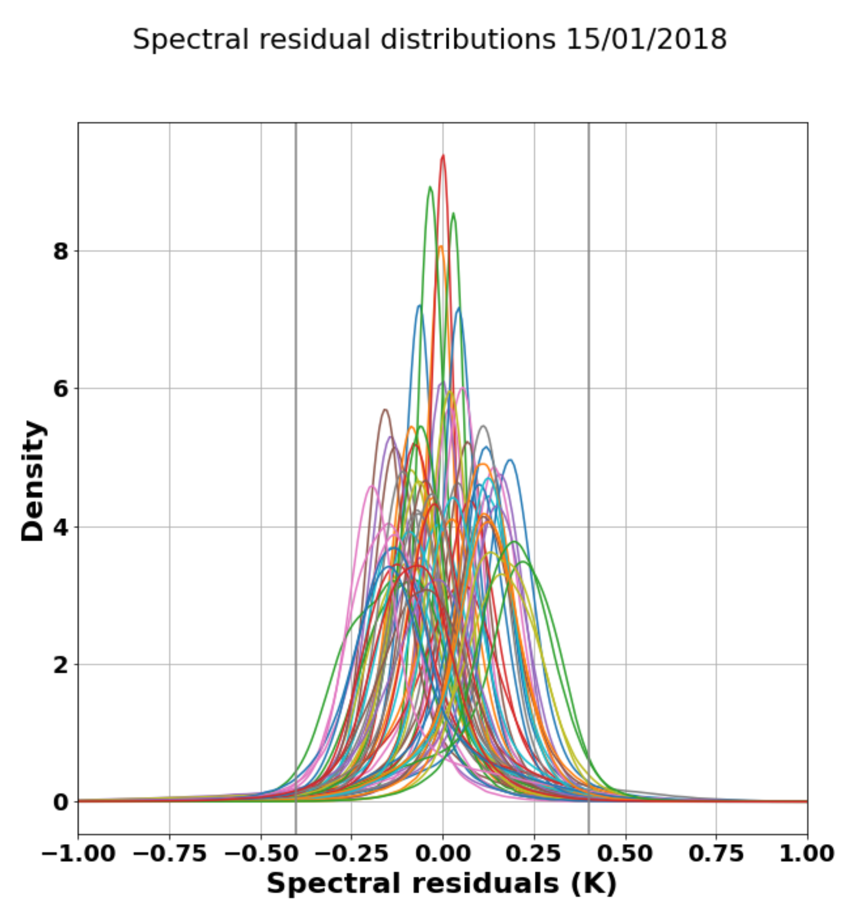

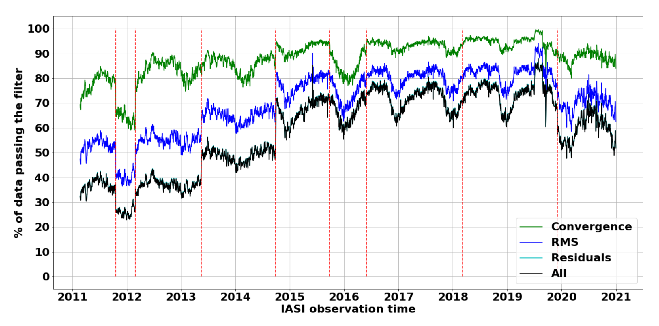
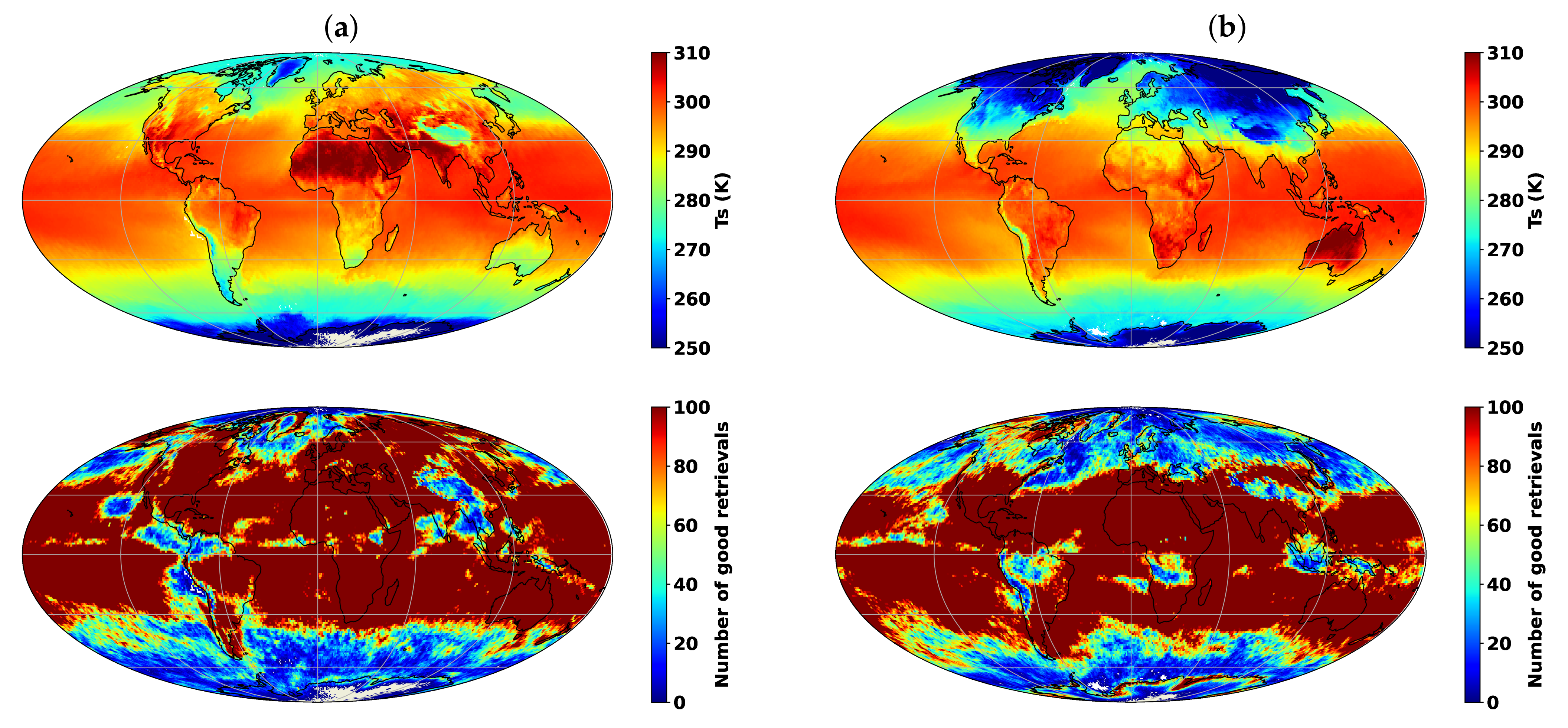
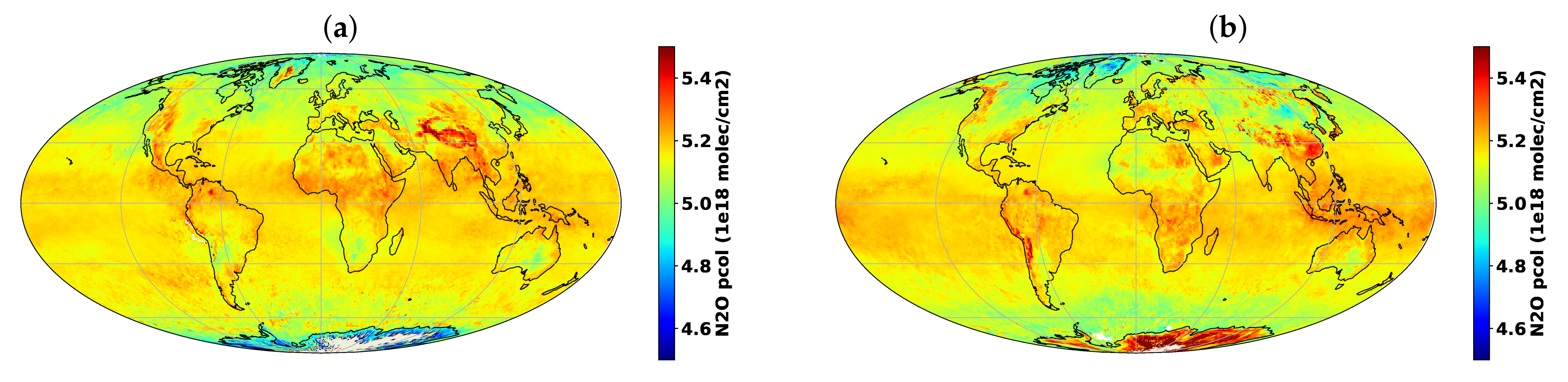
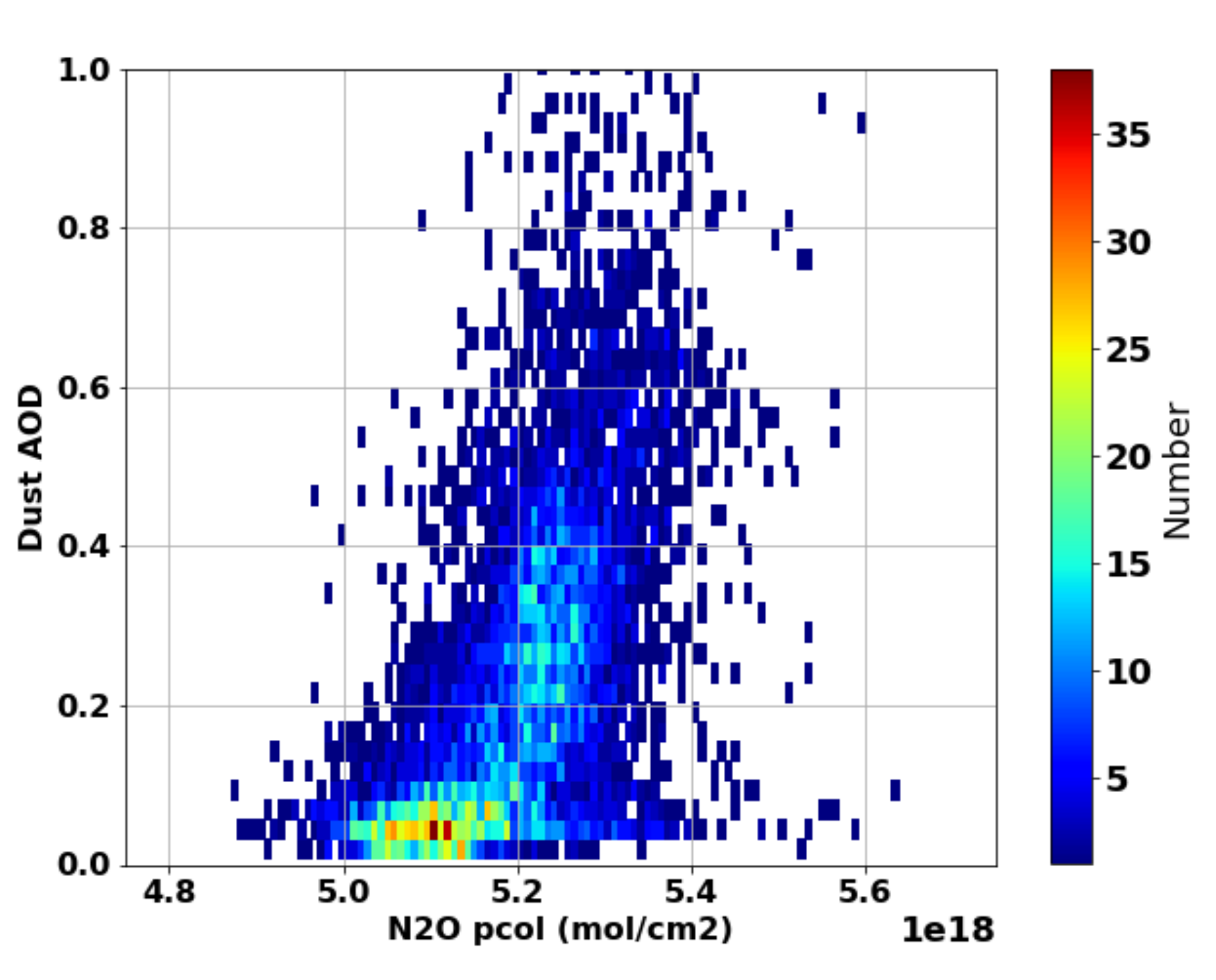
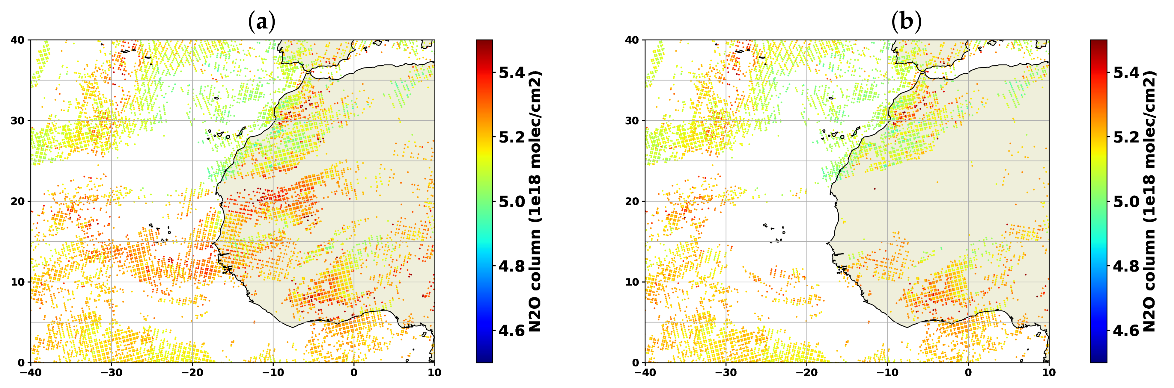
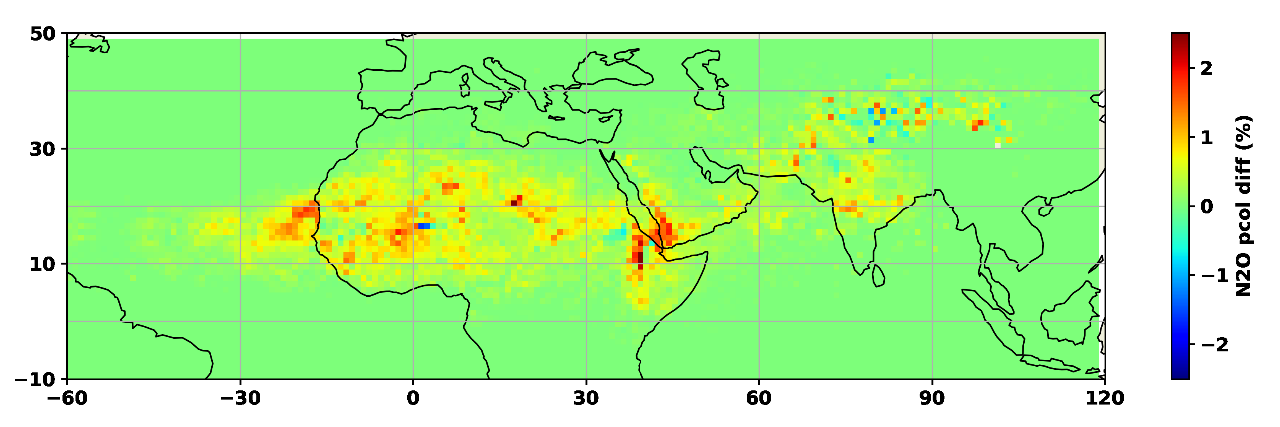
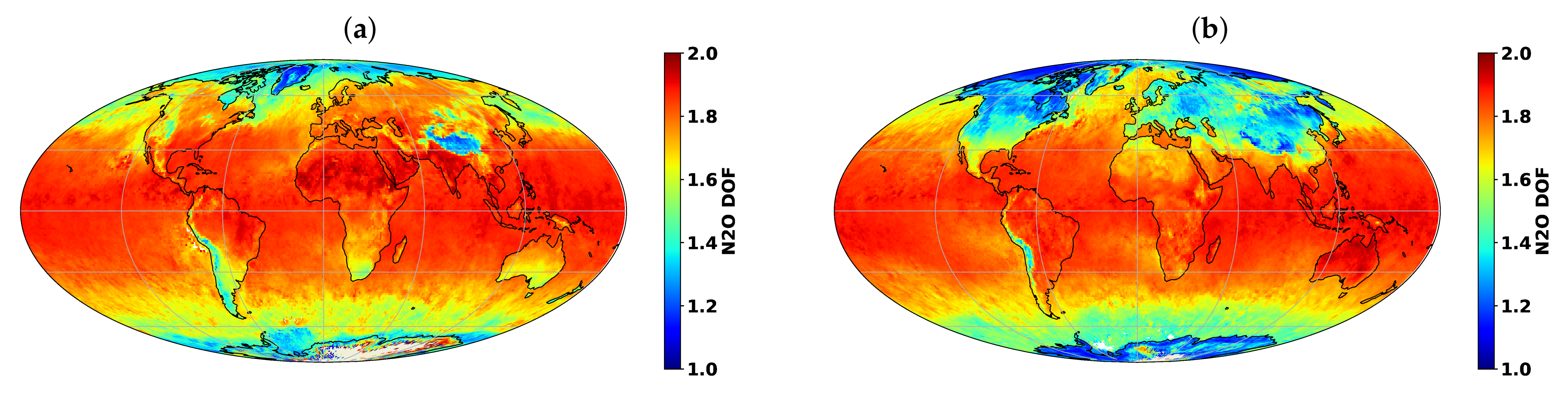
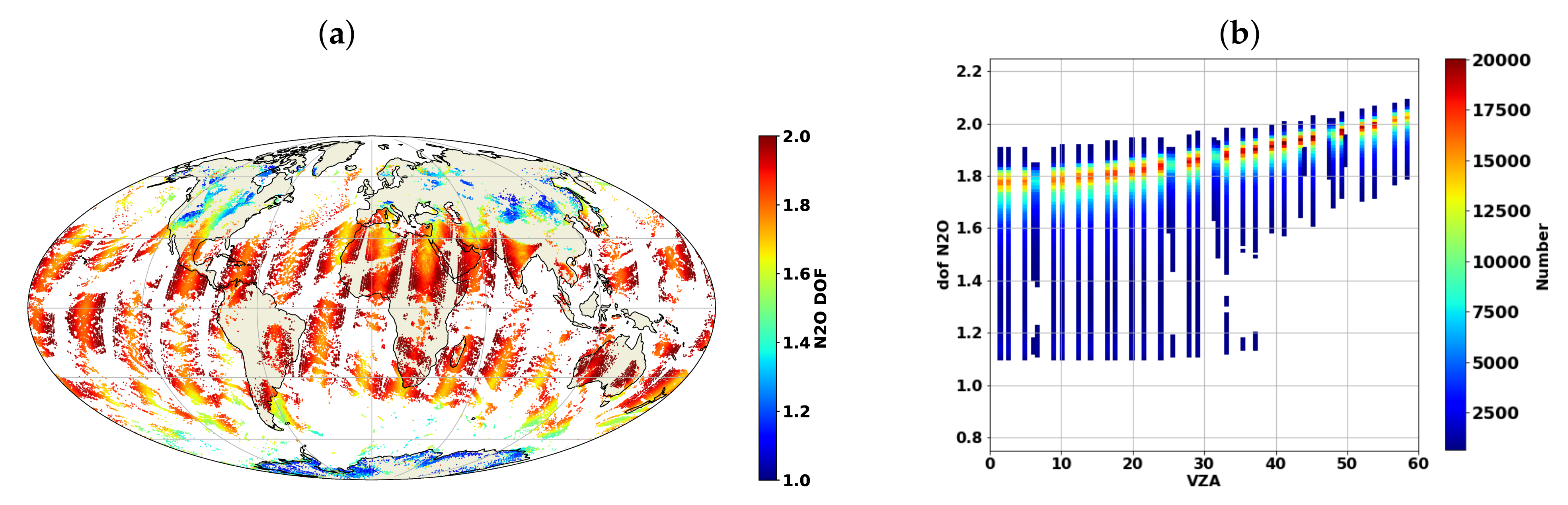

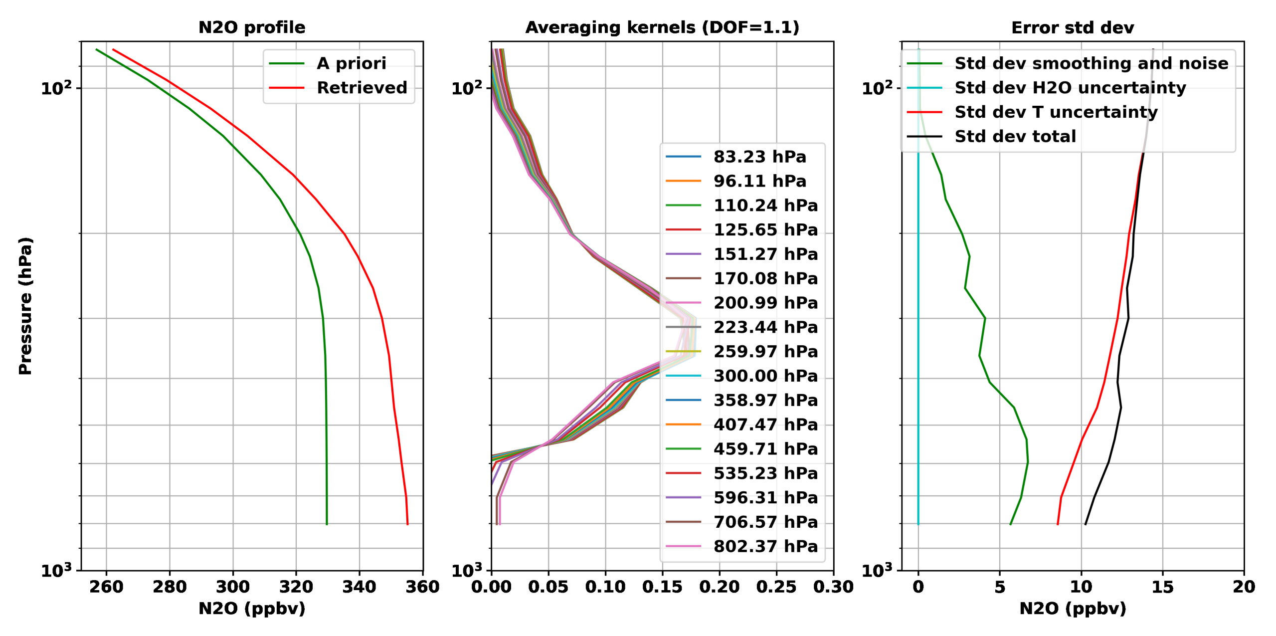
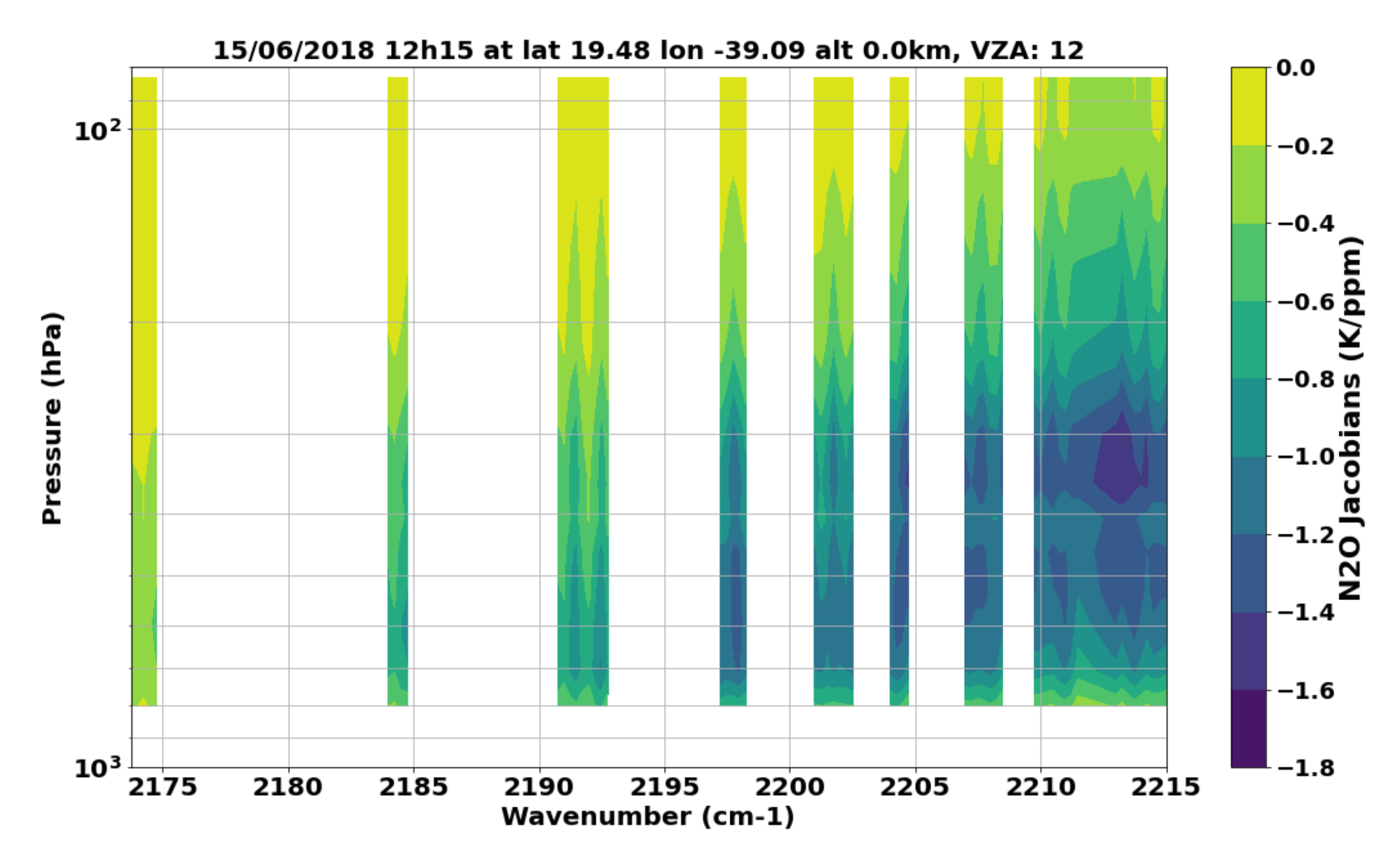
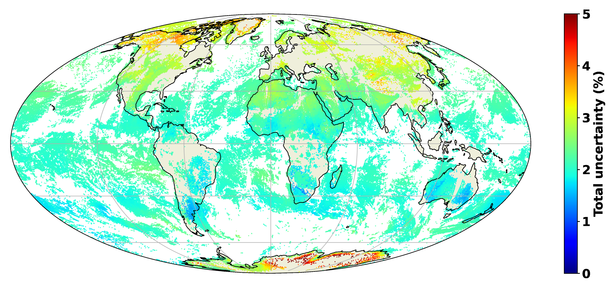

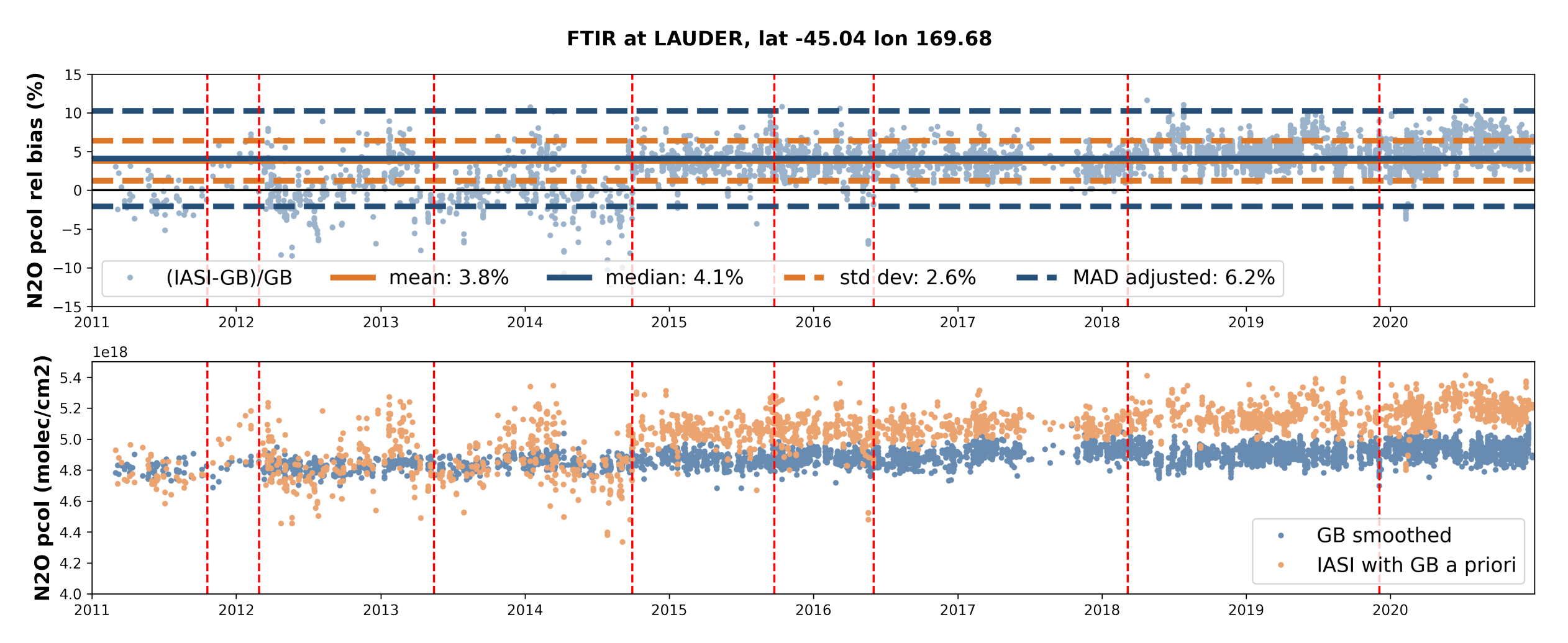
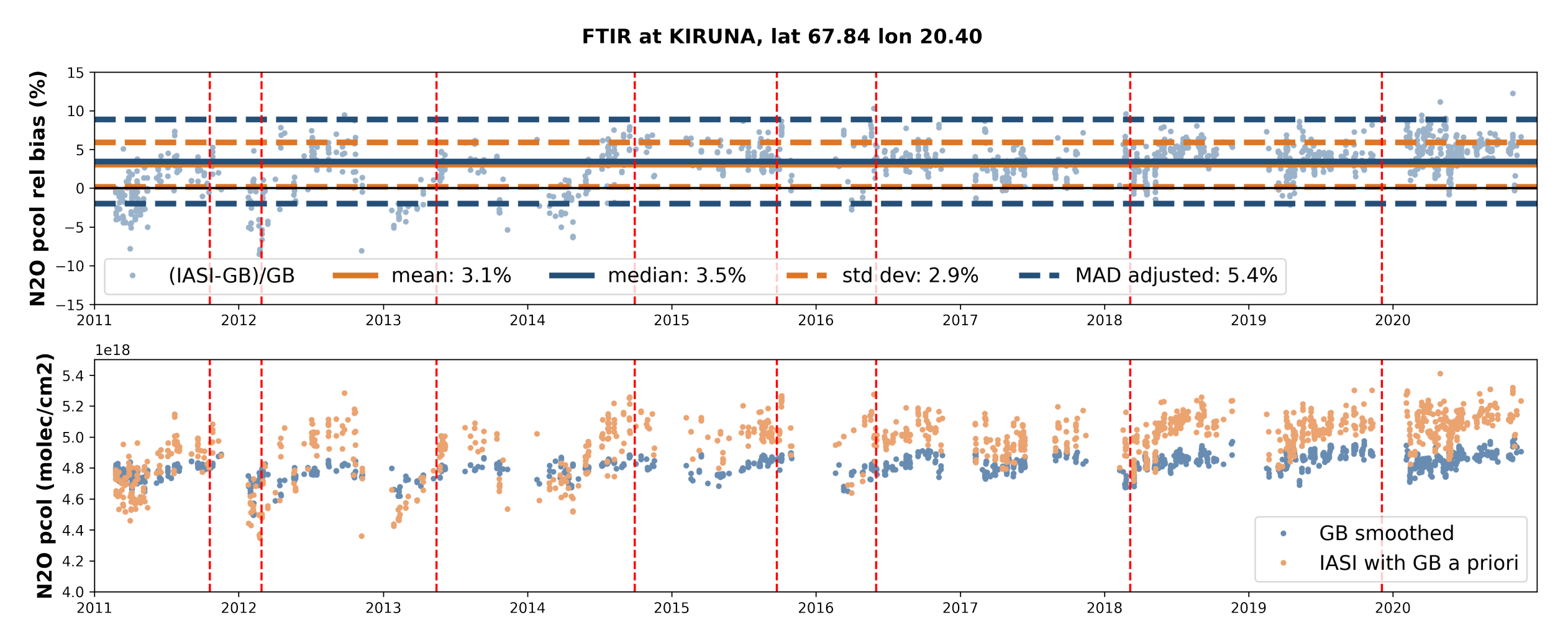


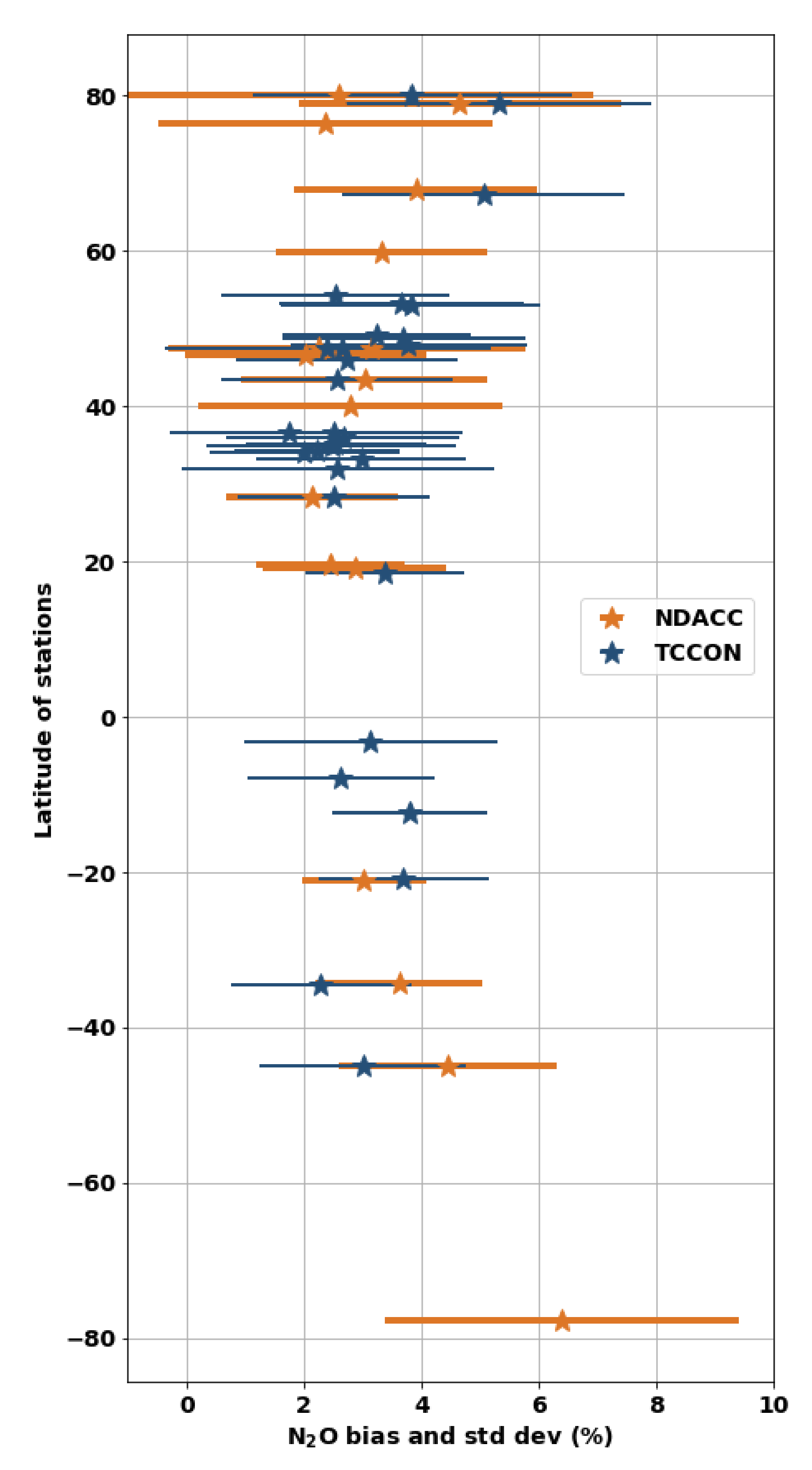
Publisher’s Note: MDPI stays neutral with regard to jurisdictional claims in published maps and institutional affiliations. |
© 2022 by the authors. Licensee MDPI, Basel, Switzerland. This article is an open access article distributed under the terms and conditions of the Creative Commons Attribution (CC BY) license (https://creativecommons.org/licenses/by/4.0/).