
Full-Resolution Quality Assessment for Pansharpening


Abstract
:
1. Introduction
- (i)
- reference-based reduced-resolution assessment (synthesis check);
- (ii)
- no-reference full-resolution assessment (consistency check).
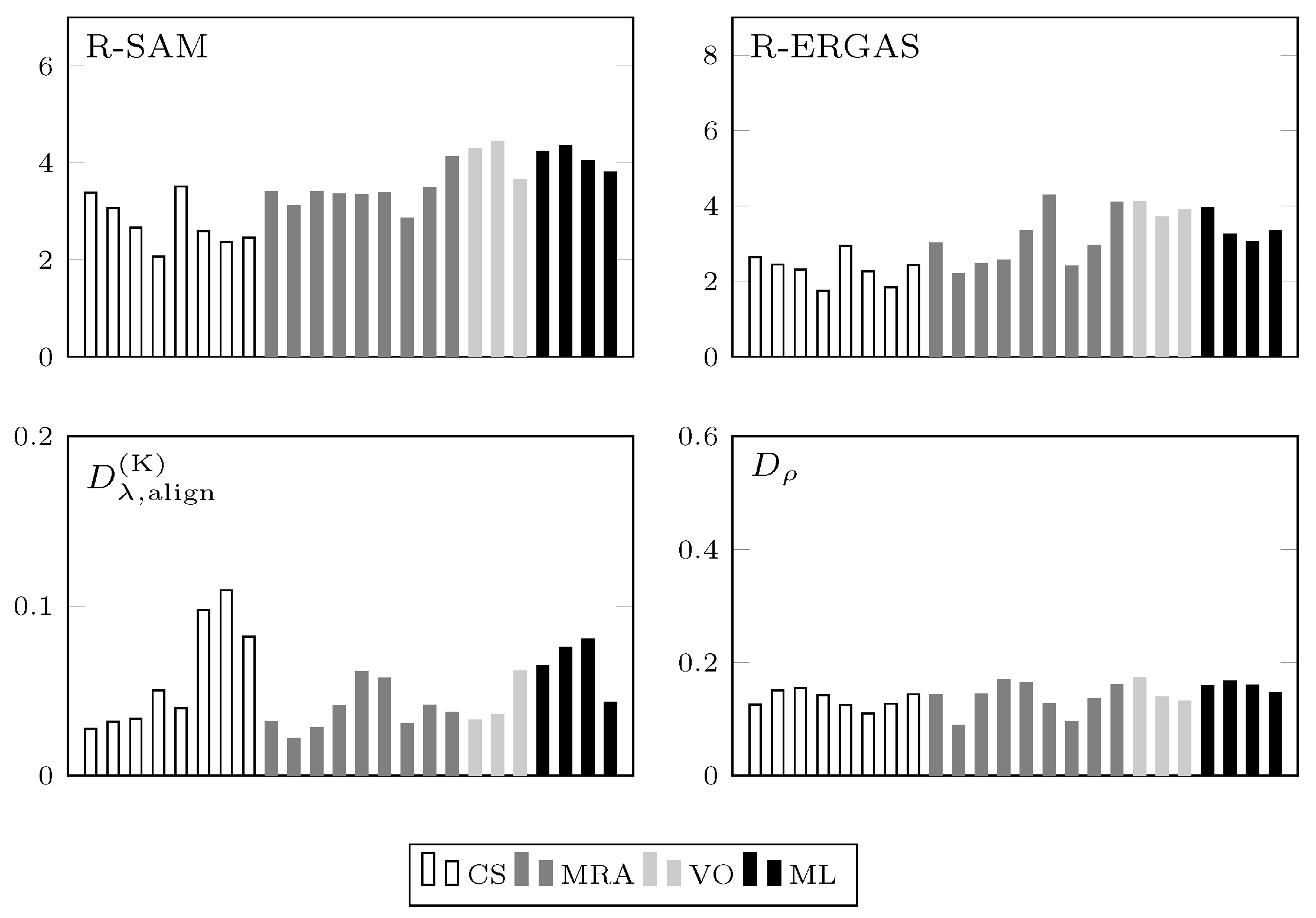
2. A Review of Panshapening Indexes
2.1. Reduced-Resolution Assessment
- (a)
- SAM (Spectral Angle Mapper) [66]. It determines the spectral similarity in terms of the pixel-wise average angle between spectral signatures. If and are two corresponding pixel spectral responses to be compared, SAM is obtained by averaging over all image locations the following “angle” among vectors:
- (b)
- ERGAS (Erreur Relative Globale Adimensionnelle de Synthése) [68]. This is one of the most popular indexes to assess both spectral and structural fidelity between a synthesized image and a target GT. Such an index presents interesting invariance properties. Indeed, it is insensitive to the radiometric range, number of bands, and resolution ratio. If B is the number of spectral bands, it is defined aswhere is the root mean square error over the b-th spectral band, and is the average intensity of the b-th band of the GT image.
- (c)
- [71]. This is a multiband extension of the universal image quality index (UIQI) [69]. Each pixel of an image with B spectral bands is accommodated into a hypercomplex (HC) number with one real part and B– 1 imaginary parts. Let and denote the HC representations of a generic GT pixel and its prediction, respectively, and then can be written as the product of three terms:The first factor provides the modulus of the HC correlation coefficient between and . The second and the third terms measure contrast changes and mean bias, respectively, on all bands simultaneously. Statistics are typically computed on 32 × 32 pixel blocks, and an average over the blocks of the whole image provides the global score, which takes values in the interval, being 1 the optimal value achieved if and only if in each location.
2.2. Full-Resolution No-Reference Assessment
- (a)
- dependence on the accuracy of the estimated MTF;
- (b)
- sensitivity to the PAN-MS alignment.
- no direct comparison between the pansharpened image and the PAN P;
- a cross-scale invariance assumption for which there are no guarantees.
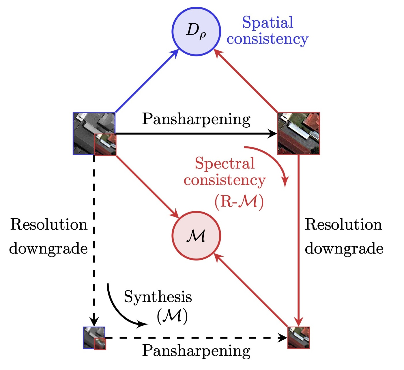
3. Proposed Full-Resolution Indexes
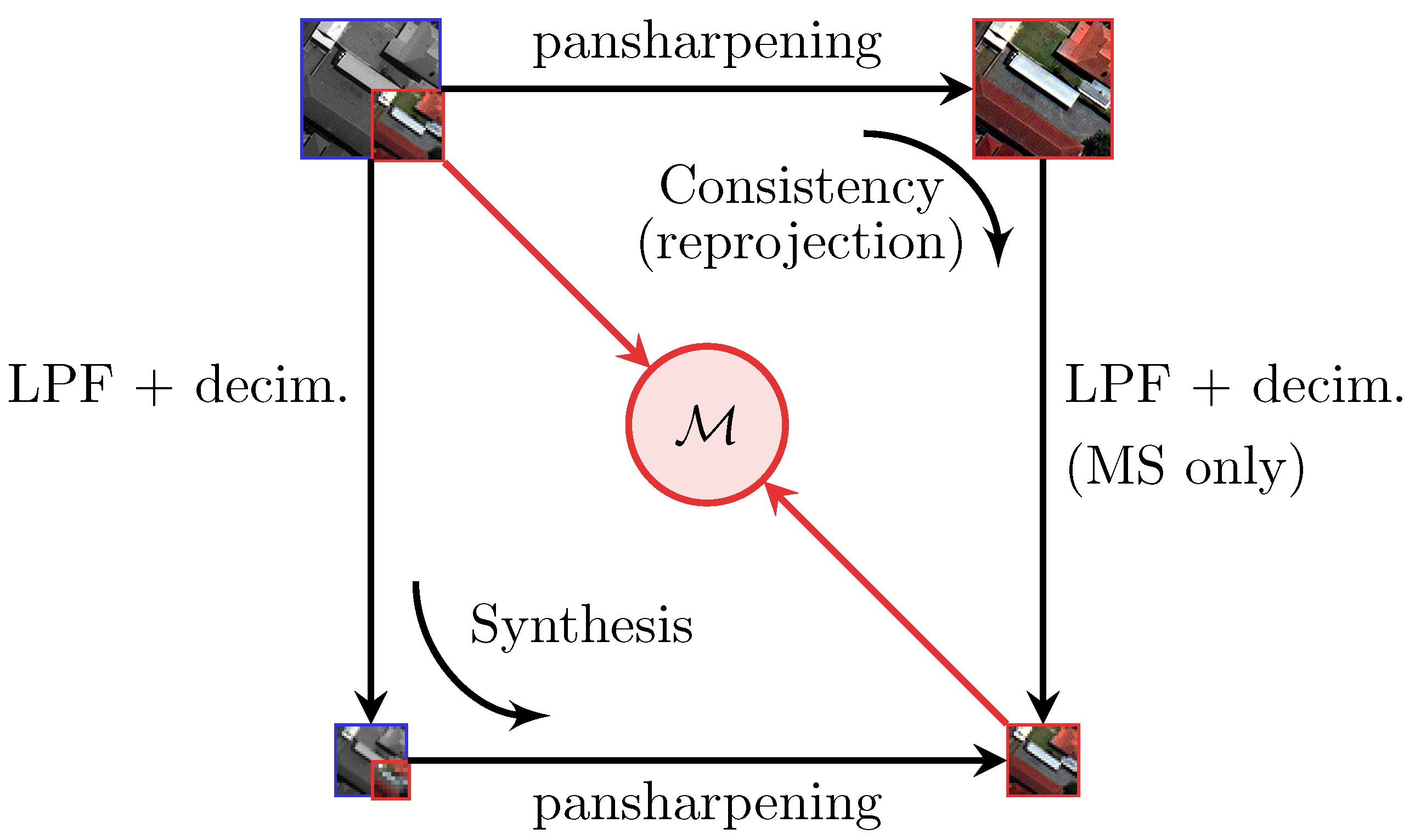
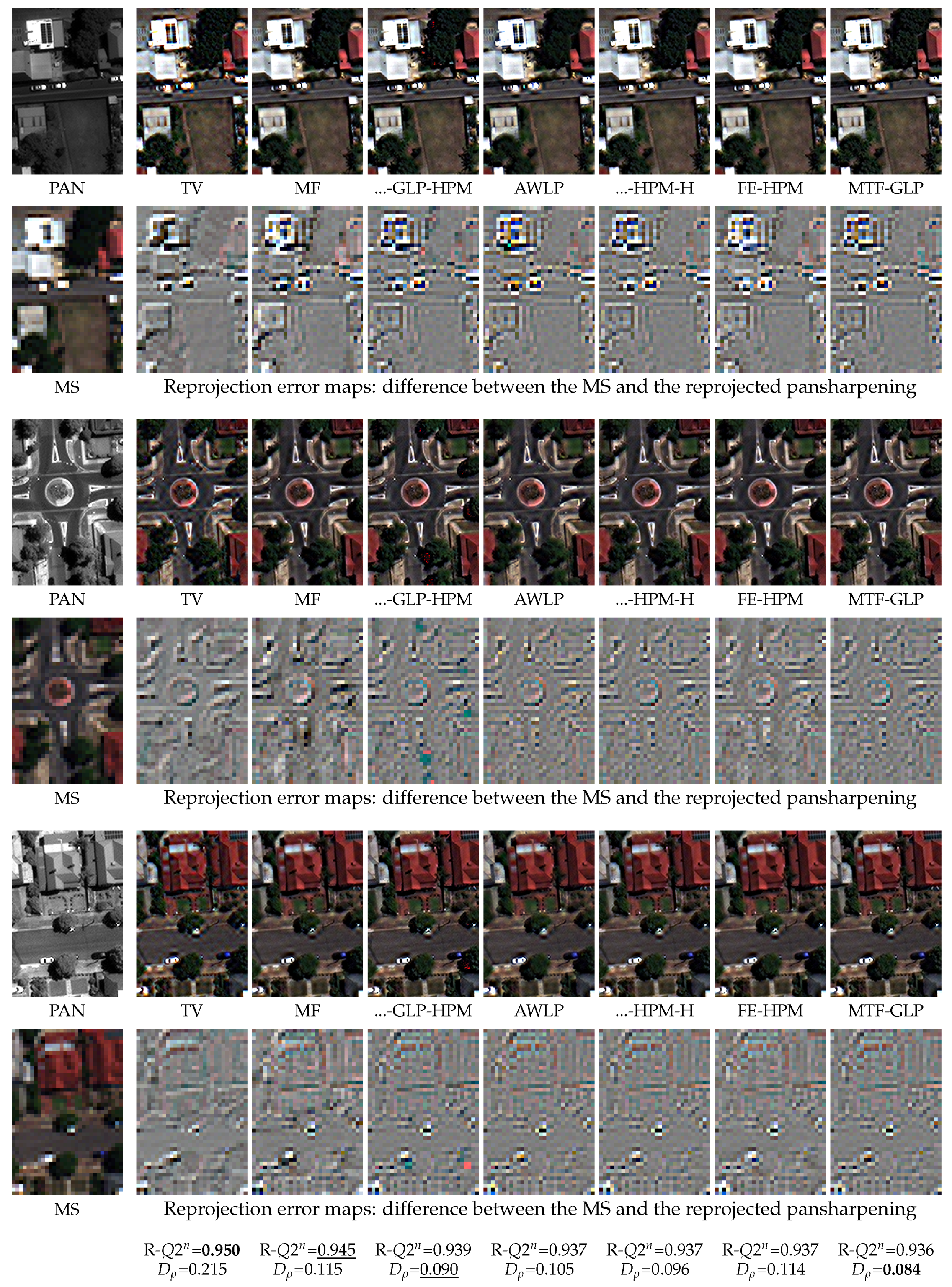
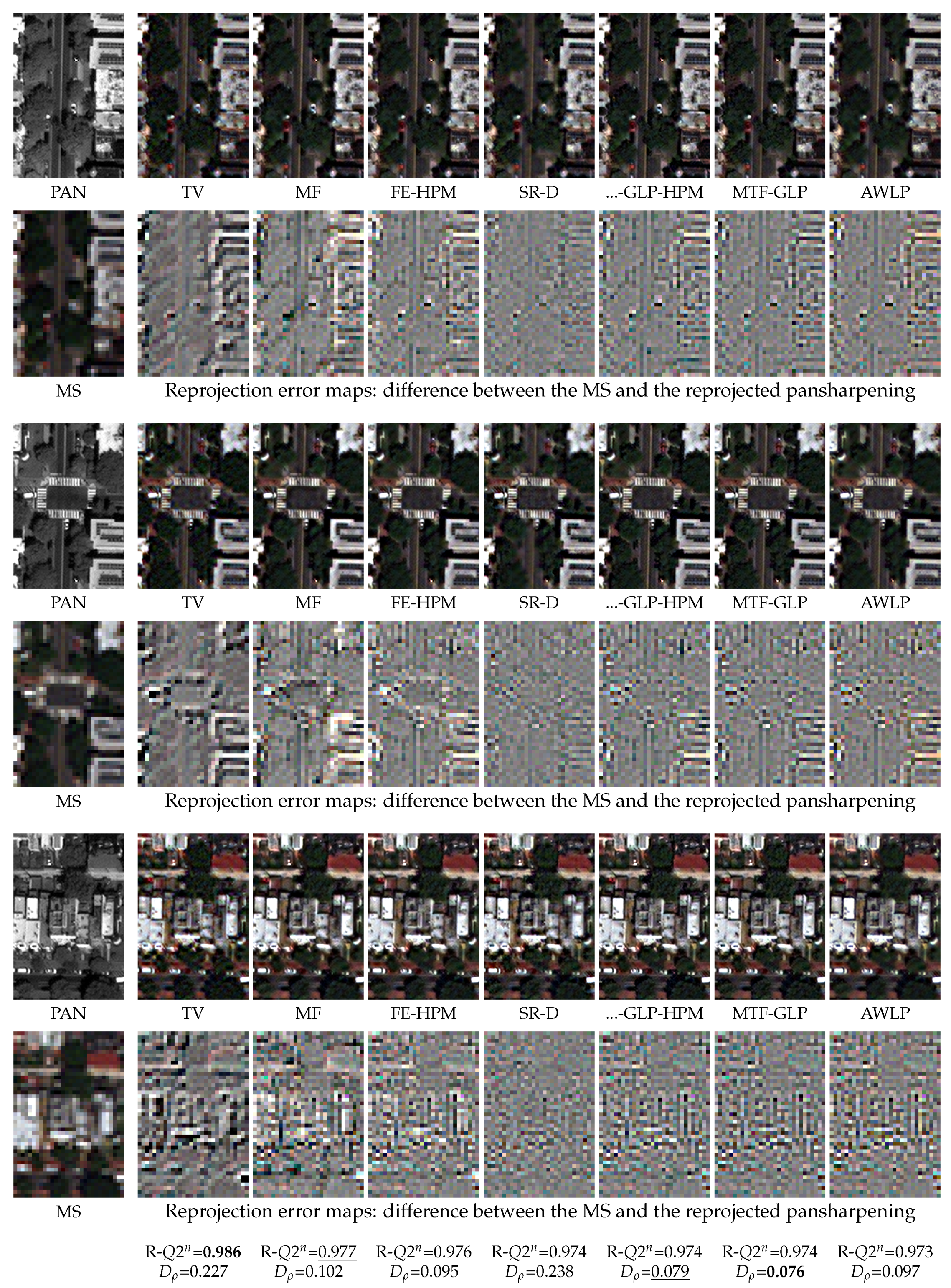
3.1. Reprojection Protocol for Spectral Accuracy Assessment
| Algorithm 1 Reprojection error assessment |
|
3.2. Correlation-Based Spatial Consistency Index
4. Experimental Results and Discussion
4.1. Datasets and Methods
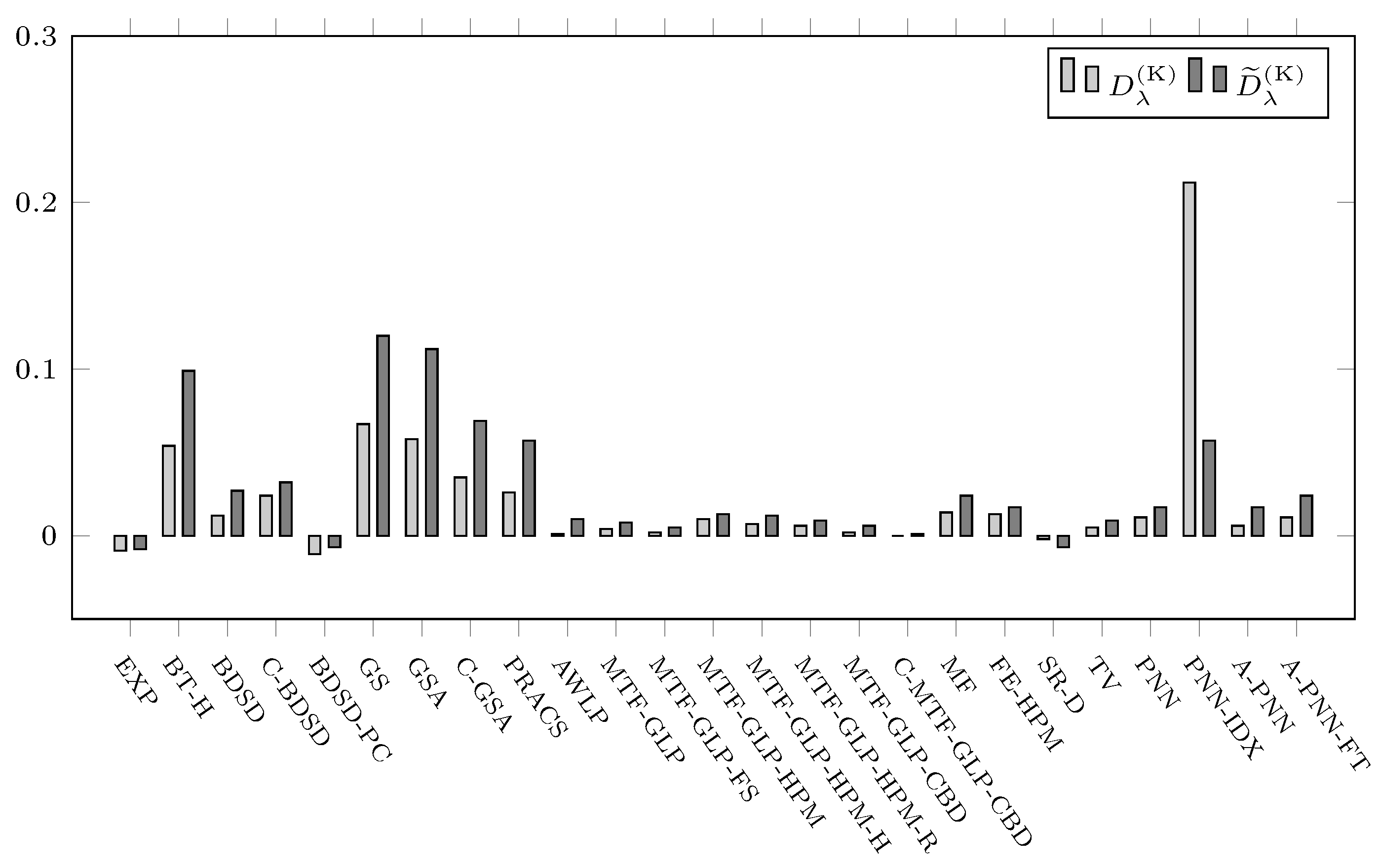
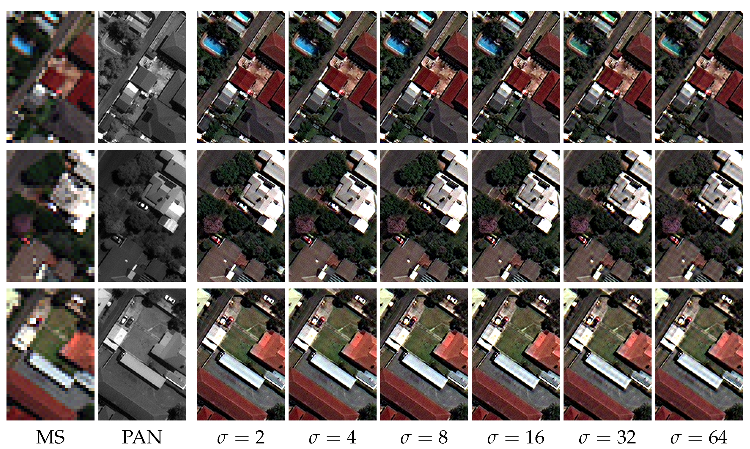
4.2. Spectral Distortion Dependence on PAN-MS Misalignment
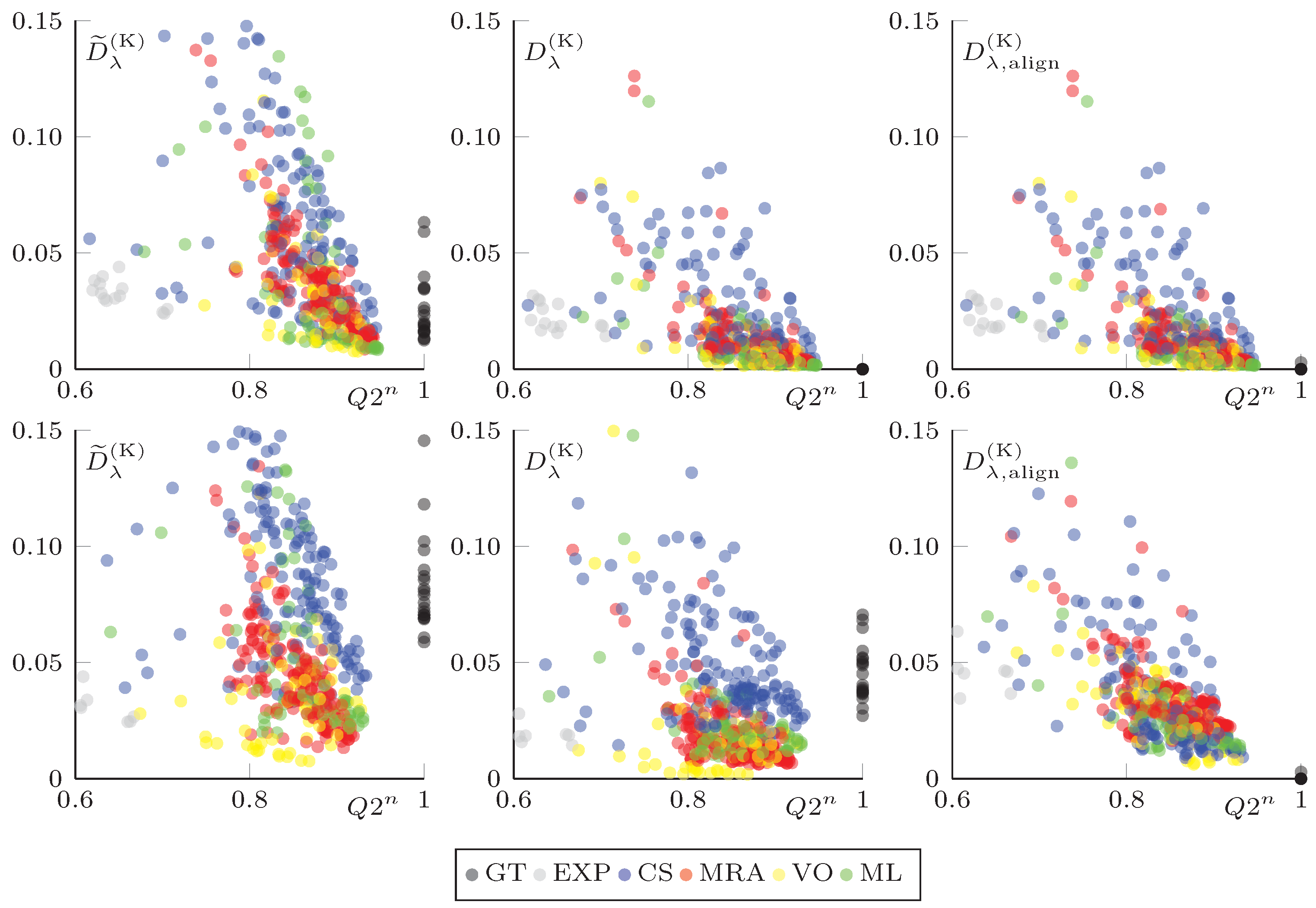
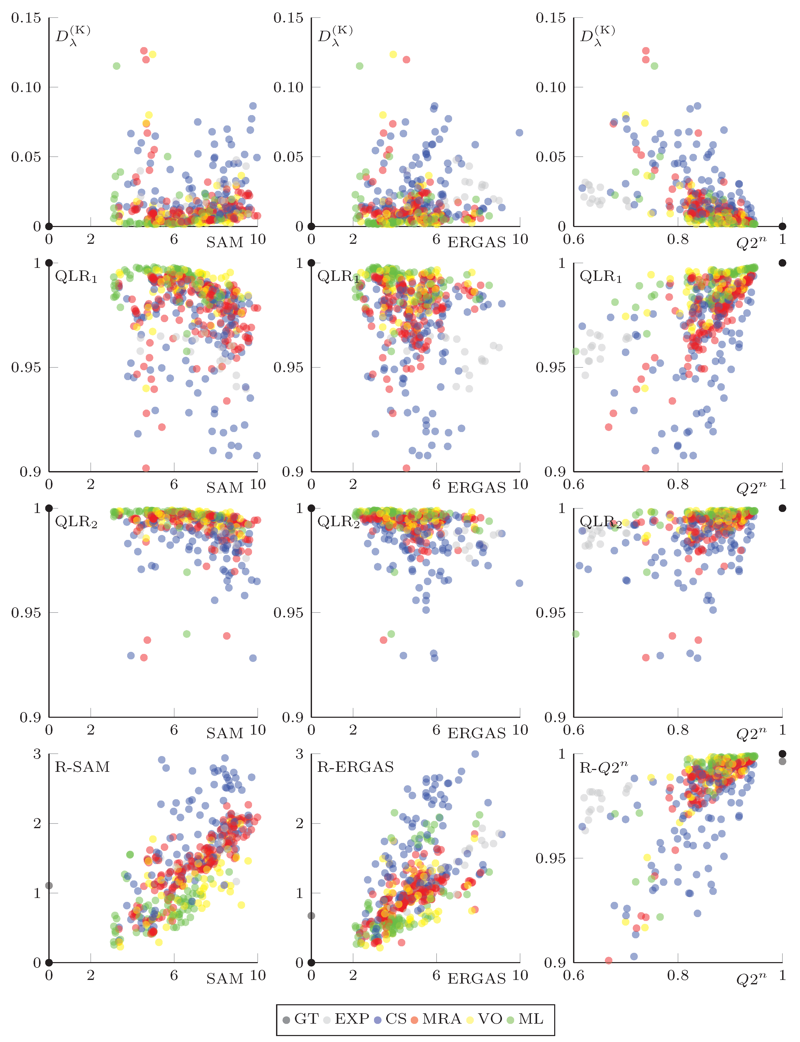
4.3. Reference vs. No-Reference Index Cross-Checking in the Reduced-Resolution Space
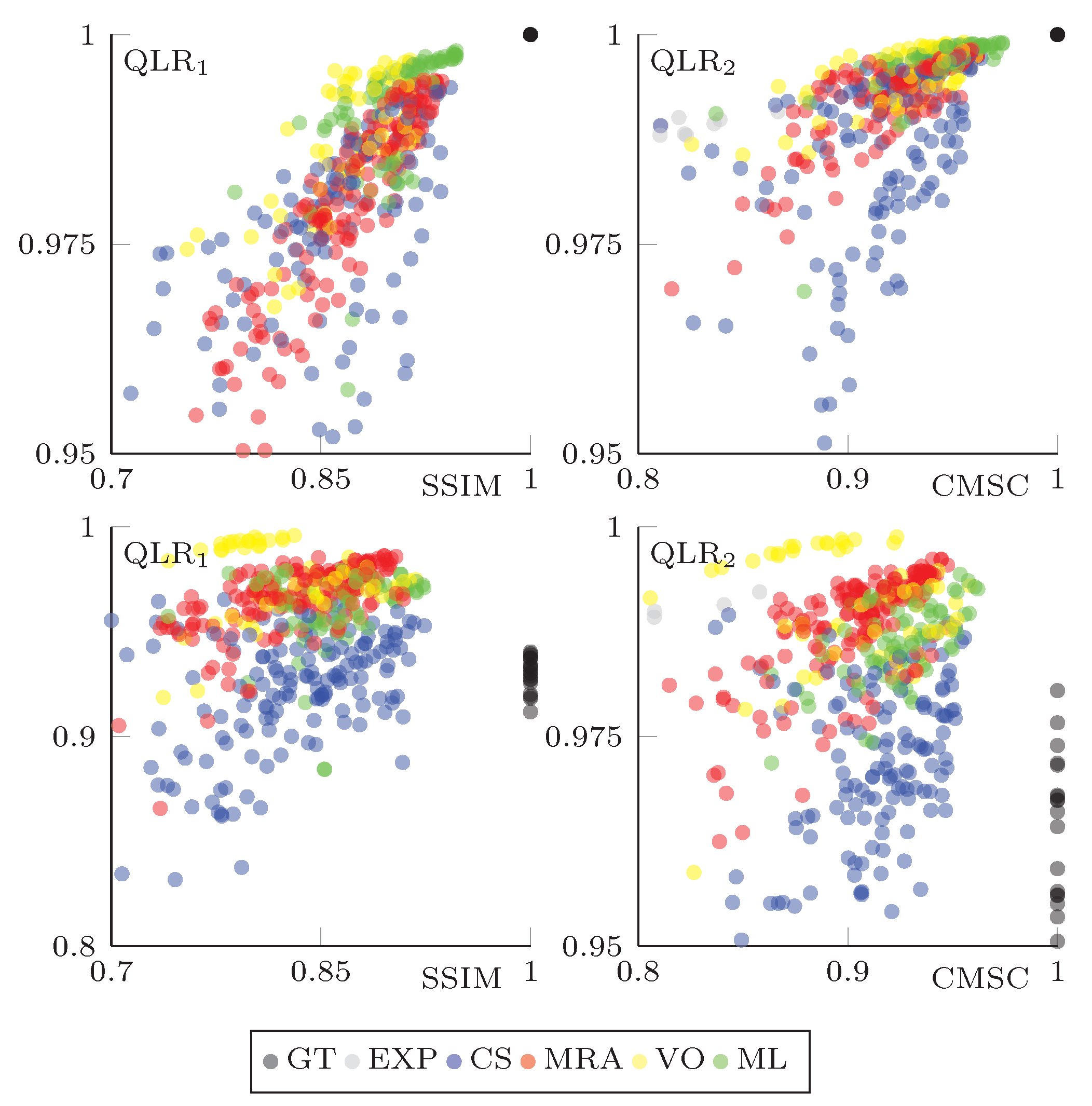
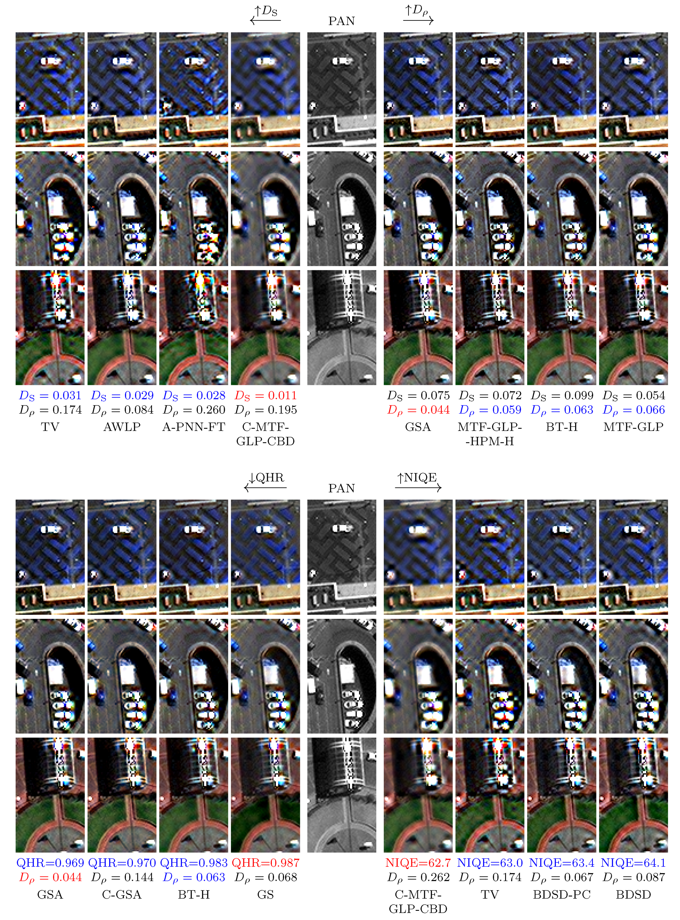
4.4. A Qualitative Assessment of the Proposed Spatial Distortion Index
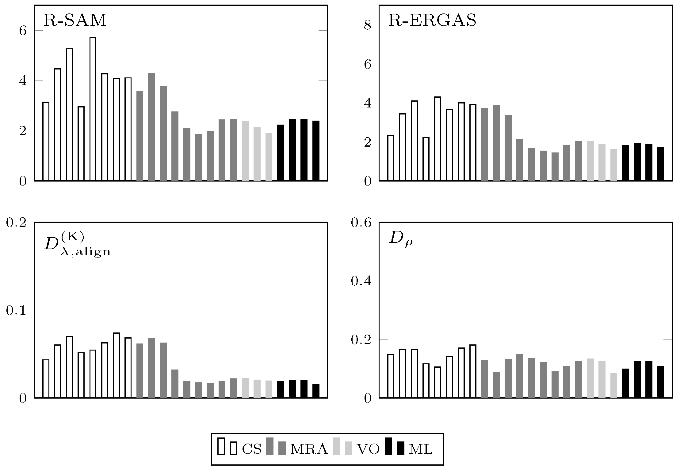
4.5. Comparative Results
5. Conclusions
Author Contributions
Funding
Data Availability Statement
Acknowledgments
Conflicts of Interest
Abbreviations
| MS | Multispectral |
| PAN | Panchromatic |
| GT | Ground Truth |
| CS | Component Substitution |
| MRA | Multiresolution Analysis |
| VO | Variational Optimization |
| ML | Machine Learning |
| IHS | Intensity–Hue–Saturation |
| GIHS | Generalized IHS |
| GS | Gram–Schmidt |
| PRACS | Partial Replacement Adaptive Component Substitution |
| BSDS | Band-Dependent Spatial-Detail |
| RR | Reduced-Resolution |
| FR | Full-Resolution |
| SAM | Spectral Angle Mapper |
| ERGAS | Erreur Relative Globale Adimensionnelle de Synthése |
| RMSE | Root Mean Squared Error |
| HC | HyperComplex |
| LPF | Low-Pass Filter |
| UIQI | Universal Image Quality Index |
| WV2 | WorldView-2 |
| WV3 | WorldView-3 |
| GSD | Ground Sample Distance |
| SSIM | Structural SIMilarity |
| QLR | Quality Low Resolution |
| QHR | Quality High Resolution |
| NIQE | Natural Image Quality Evaluator |
References
- Vivone, G.; Dalla Mura, M.; Garzelli, A.; Restaino, R.; Scarpa, G.; Ulfarsson, M.O.; Alparone, L.; Chanussot, J. A New Benchmark Based on Recent Advances in Multispectral Pansharpening: Revisiting pansharpening with classical and emerging pansharpening methods. IEEE Geosci. Remote Sens. Mag. 2020, 9, 53–81. [Google Scholar] [CrossRef]
- Shettigara, V. A generalized component substitution technique for spatial enhancement of multispectral images using a higher resolution data set. Photogramm. Eng. Remote Sens. 1992, 58, 561–567. [Google Scholar]
- Ranchin, T.; Wald, L. Fusion of high spatial and spectral resolution images: The ARSIS concept and its implementation. Photogramm. Eng. Remote Sens. 2000, 66, 49–61. [Google Scholar]
- Vivone, G.; Simões, M.; Dalla Mura, M.; Restaino, R.; Bioucas-Dias, J.M.; Licciardi, G.A.; Chanussot, J. Pansharpening Based on Semiblind Deconvolution. IEEE Trans. Geosci. Remote Sens. 2015, 53, 1997–2010. [Google Scholar] [CrossRef]
- Palsson, F.; Ulfarsson, M.O.; Sveinsson, J.R. Model-Based Reduced-Rank Pansharpening. IEEE Geosci. Remote Sens. Lett. 2020, 17, 656–660. [Google Scholar] [CrossRef]
- Masi, G.; Cozzolino, D.; Verdoliva, L.; Scarpa, G. Pansharpening by Convolutional Neural Networks. Remote Sens. 2016, 8, 594. [Google Scholar] [CrossRef] [Green Version]
- Yang, J.; Fu, X.; Hu, Y.; Huang, Y.; Ding, X.; Paisley, J. PanNet: A Deep Network Architecture for Pan-Sharpening. In Proceedings of the IEEE International Conference on Computer Vision, Venice, Italy, 22–29 October 2017. [Google Scholar] [CrossRef]
- Tu, T.M.; Su, S.C.; Shyu, H.C.; Huang, P.S. A new look at IHS-like image fusion methods. Inf. Fusion 2001, 2, 177–186. [Google Scholar] [CrossRef]
- Tu, T.M.; Huang, P.S.; Hung, C.L.; Chang, C.P. A fast intensity hue-saturation fusion technique with spectral adjustment for IKONOS imagery. IEEE Geosci. Remote Sens. Lett. 2004, 1, 309–312. [Google Scholar] [CrossRef]
- Chavez, P.; Kwarteng, A. Extracting spectral contrast in Landsat thematic mapper image data using selective principal component analysis. Photogramm. Eng. Remote Sens. 1989, 55, 339–348. [Google Scholar]
- Gillespie, A.R.; Kahle, A.B.; Walker, R.E. Color enhancement of highly correlated images. II. Channel ratio and “chromaticity” transformation techniques. Remote Sens. Environ. 1987, 22, 343–365. [Google Scholar] [CrossRef]
- Laben, C.; Brower, B. Process for Enhancing the Spatial Resolution of Multispectral Imagery Using Pan-Sharpening. U.S. Patent 6011875, 4 January 2000. [Google Scholar]
- Aiazzi, B.; Baronti, S.; Selva, M. Improving component substitution pansharpening through multivariate regression of MS+Pan data. IEEE Trans. Geosci. Remote Sens. 2007, 45, 3230–3239. [Google Scholar] [CrossRef]
- Choi, J.; Yu, K.; Kim, Y. A New Adaptive Component-Substitution-Based Satellite Image Fusion by Using Partial Replacement. IEEE Trans. Geosci. Remote Sens. 2011, 49, 295–309. [Google Scholar] [CrossRef]
- Garzelli, A.; Nencini, F.; Capobianco, L. Optimal MMSE pan sharpening of very high resolution multispectral images. IEEE Trans. Geosci. Remote Sens. 2008, 46, 228–236. [Google Scholar] [CrossRef]
- Garzelli, A. Pansharpening of Multispectral Images Based on Nonlocal Parameter Optimization. IEEE Trans. Geosci. Remote Sens. 2015, 53, 2096–2107. [Google Scholar] [CrossRef]
- Vivone, G. Robust Band-Dependent Spatial-Detail Approaches for Panchromatic Sharpening. IEEE Trans. Geosci. Remote Sens. 2019, 57, 6421–6433. [Google Scholar] [CrossRef]
- Nunez, J.; Otazu, X.; Fors, O.; Prades, A.; Pala, V.; Arbiol, R. Multiresolution-based image fusion with additive wavelet decomposition. IEEE Trans. Geosci. Remote Sens. 1999, 37, 1204–1211. [Google Scholar] [CrossRef] [Green Version]
- Otazu, X.; Gonzalez-Audicana, M.; Fors, O.; Nunez, J. Introduction of sensor spectral response into image fusion methods. Application to wavelet-based methods. IEEE Trans. Geosci. Remote Sens. 2005, 43, 2376–2385. [Google Scholar] [CrossRef] [Green Version]
- Khan, M.; Chanussot, J.; Condat, L.; Montanvert, A. Indusion: Fusion of Multispectral and Panchromatic Images Using the Induction Scaling Technique. IEEE Geosci. Remote Sens. Lett. 2008, 5, 98–102. [Google Scholar] [CrossRef] [Green Version]
- Aiazzi, B.; Alparone, L.; Baronti, S.; Garzelli, A. Context-driven fusion of high spatial and spectral resolution images based on oversampled multiresolution analysis. IEEE Trans. Geosci. Remote Sens. 2002, 40, 2300–2312. [Google Scholar] [CrossRef]
- Aiazzi, B.; Alparone, L.; Baronti, S.; Garzelli, A.; Selva, M. An MTF-based spectral distortion minimizing model for pan-sharpening of very high resolution multispectral images of urban areas. In Proceedings of the GRSS/ISPRS Joint Workshop on Remote Sensing and Data Fusion over Urban Areas, Berlin, Germany, 22–23 May 2003; pp. 90–94. [Google Scholar]
- Aiazzi, B.; Alparone, L.; Baronti, S.; Garzelli, A.; Selva, M. MTF-tailored multiscale fusion of high-resolution MS and Pan imagery. Photogramm. Eng. Remote Sens. 2006, 72, 591–596. [Google Scholar] [CrossRef]
- Lee, J.; Lee, C. Fast and Efficient Panchromatic Sharpening. IEEE Trans. Geosci. Remote Sens. 2010, 48, 155–163. [Google Scholar] [CrossRef]
- Restaino, R.; Mura, M.D.; Vivone, G.; Chanussot, J. Context-Adaptive Pansharpening Based on Image Segmentation. IEEE Trans. Geosci. Remote Sens. 2017, 55, 753–766. [Google Scholar] [CrossRef] [Green Version]
- Shah, V.P.; Younan, N.H.; King, R.L. An Efficient Pan-Sharpening Method via a Combined Adaptive PCA Approach and Contourlets. IEEE Trans. Geosci. Remote Sens. 2008, 46, 1323–1335. [Google Scholar] [CrossRef]
- Vicinanza, M.R.; Restaino, R.; Vivone, G.; Mura, M.D.; Chanussot, J. A Pansharpening Method Based on the Sparse Representation of Injected Details. IEEE Geosci. Remote Sens. Lett. 2015, 12, 180–184. [Google Scholar] [CrossRef]
- Palsson, F.; Sveinsson, J.; Ulfarsson, M. A New Pansharpening Algorithm Based on Total Variation. IEEE Geosci. Remote Sens. Lett. 2014, 11, 318–322. [Google Scholar] [CrossRef]
- Palsson, F.; Sveinsson, J.R.; Ulfarsson, M.O.; Benediktsson, J.A. Model-Based Fusion of Multi- and Hyperspectral Images Using PCA and Wavelets. IEEE Trans. Geosci. Remote Sens. 2015, 53, 2652–2663. [Google Scholar] [CrossRef]
- Fasbender, D.; Radoux, J.; Bogaert, P. Bayesian Data Fusion for Adaptable Image Pansharpening. IEEE Trans. Geosci. Remote Sens. 2008, 46, 1847–1857. [Google Scholar] [CrossRef]
- Zhang, L.; Shen, H.; Gong, W.; Zhang, H. Adjustable Model-Based Fusion Method for Multispectral and Panchromatic Images. IEEE Trans. Syst. Man Cybern. B Cybern. 2012, 42, 1693–1704. [Google Scholar] [CrossRef]
- Meng, X.; Shen, H.; Li, H.; Yuan, Q.; Zhang, H.; Zhang, L. Improving the spatial resolution of hyperspectral image using panchromatic and multispectral images: An integrated method. In Proceedings of the 2015 7th Workshop on Hyperspectral Image and Signal Processing: Evolution in Remote Sensing (WHISPERS), Tokyo, Japan, 2–5 June 2015. [Google Scholar]
- Shen, H.; Meng, X.; Zhang, L. An Integrated Framework for the Spatio-Temporal-Spectral Fusion of Remote Sensing Images. IEEE Trans. Geosci. Remote Sens. 2016, 54, 7135–7148. [Google Scholar] [CrossRef]
- Zhong, S.; Zhang, Y.; Chen, Y.; Wu, D. Combining Component Substitution and Multiresolution Analysis: A Novel Generalized BDSD Pansharpening Algorithm. IEEE J. Sel. Top. Appl. Earth Obs. Remote Sens. 2017, 10, 2867–2875. [Google Scholar] [CrossRef]
- Li, S.; Yang, B. A New Pan-Sharpening Method Using a Compressed Sensing Technique. IEEE Trans. Geosci. Remote Sens. 2011, 49, 738–746. [Google Scholar] [CrossRef]
- Li, S.; Yin, H.; Fang, L. Remote Sensing Image Fusion via Sparse Representations Over Learned Dictionaries. IEEE Trans. Geosci. Remote Sens. 2013, 51, 4779–4789. [Google Scholar] [CrossRef]
- Zhu, X.; Bamler, R. A Sparse Image Fusion Algorithm With Application to Pan-Sharpening. IEEE Trans. Geosci. Remote Sens. 2013, 51, 2827–2836. [Google Scholar] [CrossRef]
- Cheng, M.; Wang, C.; Li, J. Sparse representation based pansharpening using trained dictionary. IEEE Geosci. Remote Sens. Lett. 2014, 11, 293–297. [Google Scholar] [CrossRef]
- Zhu, X.X.; Grohnfeldt, C.; Bamler, R. Exploiting Joint Sparsity for Pansharpening: The J-SparseFI Algorithm. IEEE Trans. Geosci. Remote Sens. 2016, 54, 2664–2681. [Google Scholar] [CrossRef] [Green Version]
- Hong, D.; Yokoya, N.; Chanussot, J.; Zhu, X.X. An Augmented Linear Mixing Model to Address Spectral Variability for Hyperspectral Unmixing. IEEE Trans. Image Process. 2019, 28, 1923–1938. [Google Scholar] [CrossRef] [Green Version]
- Yokoya, N.; Yairi, T.; Iwasaki, A. Coupled Nonnegative Matrix Factorization Unmixing for Hyperspectral and Multispectral Data Fusion. IEEE Trans. Geosci. Remote Sens. 2012, 50, 528–537. [Google Scholar] [CrossRef]
- Lanaras, C.; Baltsavias, E.; Schindler, K. Hyperspectral Super-Resolution by Coupled Spectral Unmixing. In Proceedings of the 2015 IEEE International Conference on Computer Vision (ICCV), Santiago, Chile, 7–13 December 2015; pp. 3586–3594. [Google Scholar]
- Hong, D.; Yokoya, N.; Chanussot, J.; Zhu, X.X. CoSpace: Common Subspace Learning From Hyperspectral-Multispectral Correspondences. IEEE Trans. Geosci. Remote Sens. 2019, 57, 4349–4359. [Google Scholar] [CrossRef] [Green Version]
- Vivone, G.; Alparone, L.; Chanussot, J.; Mura, M.D.; Garzelli, A.; Licciardi, G.A.; Restaino, R.; Wald, L. A Critical Comparison Among Pansharpening Algorithms. IEEE Trans. Geosci. Remote Sens. 2015, 53, 2565–2586. [Google Scholar] [CrossRef]
- Krizhevsky, A.; Sutskever, I.; Hinton, G.E. Imagenet classification with deep convolutional neural networks. In Proceedings of the Advances in Neural Information Processing Systems, Lake Tahoe, NV, USA, 3–8 December 2012; pp. 1106–1114. [Google Scholar]
- Dong, C.; Loy, C.; He, K.; Tang, X. Image Super-Resolution Using Deep Convolutional Networks. IEEE Trans. Pattern Anal. Mach. Intell. 2016, 38, 295–307. [Google Scholar] [CrossRef] [Green Version]
- He, K.; Gkioxari, G.; Dollár, P.; Girshick, R. Mask R-CNN. In Proceedings of the 2017 IEEE International Conference on Computer Vision (ICCV), Venice, Italy, 22–29 October 2017; pp. 2980–2988. [Google Scholar]
- Lateef, F.; Ruichek, Y. Survey on semantic segmentation using deep learning techniques. Neurocomputing 2019, 338, 321–348. [Google Scholar] [CrossRef]
- Zhao, Z.; Zheng, P.; Xu, S.; Wu, X. Object Detection With Deep Learning: A Review. IEEE Trans. Neural Netw. Learn. Syst. 2019, 30, 3212–3232. [Google Scholar] [CrossRef] [PubMed] [Green Version]
- Scarpa, G.; Gargiulo, M.; Mazza, A.; Gaetano, R. A CNN-Based Fusion Method for Feature Extraction from Sentinel Data. Remote Sens. 2018, 10, 236. [Google Scholar] [CrossRef] [Green Version]
- Benedetti, P.; Ienco, D.; Gaetano, R.; Ose, K.; Pensa, R.G.; Dupuy, S. M3Fusion: A Deep Learning Architecture for Multiscale Multimodal Multitemporal Satellite Data Fusion. IEEE J. Sel. Top. Appl. Earth Obs. Remote Sens. 2018, 11, 4939–4949. [Google Scholar] [CrossRef] [Green Version]
- Mazza, A.; Sica, F.; Rizzoli, P.; Scarpa, G. TanDEM-X Forest Mapping Using Convolutional Neural Networks. Remote Sens. 2019, 11, 2980. [Google Scholar] [CrossRef] [Green Version]
- Wei, Y.; Yuan, Q. Deep residual learning for remote sensed imagery pansharpening. In Proceedings of the 2017 International Workshop on Remote Sensing with Intelligent Processing (RSIP), Shanghai, China, 19–21 May 2017; pp. 1–4. [Google Scholar]
- Wei, Y.; Yuan, Q.; Shen, H.; Zhang, L. Boosting the Accuracy of Multispectral Image Pansharpening by Learning a Deep Residual Network. IEEE Geosci. Remote Sens. Lett. 2017, 14, 1795–1799. [Google Scholar] [CrossRef] [Green Version]
- Rao, Y.; He, L.; Zhu, J. A residual convolutional neural network for pan-shaprening. In Proceedings of the 2017 International Workshop on Remote Sensing with Intelligent Processing (RSIP), Shanghai, China, 19–21 May 2017; pp. 1–4. [Google Scholar]
- Masi, G.; Cozzolino, D.; Verdoliva, L.; Scarpa, G. CNN-based Pansharpening of Multi-Resolution Remote-Sensing Images. In Proceedings of the Joint Urban Remote Sensing Event 2017, Dubai, United Arab Emirates, 6–8 March 2017. [Google Scholar]
- Azarang, A.; Ghassemian, H. A new pansharpening method using multi resolution analysis framework and deep neural networks. In Proceedings of the 2017 3rd International Conference on Pattern Recognition and Image Analysis (IPRIA), Shahrekord, Iran, 19–20 April 2017; pp. 1–6. [Google Scholar]
- Yuan, Q.; Wei, Y.; Meng, X.; Shen, H.; Zhang, L. A Multiscale and Multidepth Convolutional Neural Network for Remote Sensing Imagery Pan-Sharpening. IEEE J. Sel. Top. Appl. Earth Obs. Remote Sens. 2018, 11, 978–989. [Google Scholar] [CrossRef] [Green Version]
- Liu, X.; Wang, Y.; Liu, Q. Psgan: A Generative Adversarial Network for Remote Sensing Image Pan-Sharpening. In Proceedings of the 2018 25th IEEE International Conference on Image Processing (ICIP), Athens, Greece, 7–10 October 2018; pp. 873–877. [Google Scholar]
- Shao, Z.; Cai, J. Remote Sensing Image Fusion With Deep Convolutional Neural Network. IEEE J. Sel. Top. Appl. Earth Observ. 2018, 11, 1656–1669. [Google Scholar] [CrossRef]
- Vitale, S.; Ferraioli, G.; Scarpa, G. A CNN-Based Model for Pansharpening of WorldView-3 Images. In Proceedings of the IGARSS 2018—2018 IEEE International Geoscience and Remote Sensing Symposium, Valencia, Spain, 22–27 July 2018; pp. 5108–5111. [Google Scholar] [CrossRef]
- Zhang, Y.; Liu, C.; Sun, M.; Ou, Y. Pan-Sharpening Using an Efficient Bidirectional Pyramid Network. IEEE Trans. Geosci. Remote Sens. 2019, 57, 5549–5563. [Google Scholar] [CrossRef]
- Dong, W.; Zhang, T.; Qu, J.; Xiao, S.; Liang, J.; Li, Y. Laplacian Pyramid Dense Network for Hyperspectral Pansharpening. IEEE Trans. Geosci. Remote Sens. 2021, 60, 1–13. [Google Scholar] [CrossRef]
- Dong, W.; Hou, S.; Xiao, S.; Qu, J.; Du, Q.; Li, Y. Generative Dual-Adversarial Network With Spectral Fidelity and Spatial Enhancement for Hyperspectral Pansharpening. IEEE Trans. Neural Netw. Learn. Syst. 2021, 1–15. [Google Scholar] [CrossRef] [PubMed]
- Wald, L.; Ranchin, T.; Mangolini, M. Fusion of satellite images of different spatial resolution: Assessing the quality of resulting images. Photogramm. Eng. Remote Sens. 1997, 63, 691–699. [Google Scholar]
- Kruse, F.A.; Lefkoff, A.; Boardman, J.; Heidebrecht, K.; Shapiro, A.; Barloon, P.; Goetz, A. The spectral image processing system (SIPS)—interactive visualization and analysis of imaging spectrometer data. Remote Sens. Environ. 1993, 44, 145–163. [Google Scholar] [CrossRef]
- Zhou, J.; Civco, D.L.; Silander, J.A. A wavelet transform method to merge Landsat TM and SPOT panchromatic data. Int. J. Remote Sens. 1998, 19, 743–757. [Google Scholar] [CrossRef]
- Wald, L. Quality of high resolution synthesised images: Is there a simple criterion? In Proceedings of the Third conference “Fusion of Earth Data: Merging Point Measurements, Raster Maps and Remotely Sensed Images”. SEE/URISCA, Sophia Antipolis, France, 26–28 January 2000; pp. 99–103. [Google Scholar]
- Wang, Z.; Bovik, A.C. A universal image quality index. IEEE Signal Process. Lett. 2002, 9, 81–84. [Google Scholar] [CrossRef]
- Alparone, L.; Baronti, S.; Garzelli, A.; Nencini, F. A global quality measurement of pan-sharpened multispectral imagery. IEEE Geosci. Remote Sens. Lett. 2004, 1, 313–317. [Google Scholar] [CrossRef]
- Garzelli, A.; Nencini, F. Hypercomplex Quality Assessment of Multi/Hyperspectral Images. IEEE Geosci. Remote Sens. Lett. 2009, 6, 662–665. [Google Scholar] [CrossRef]
- Alparone, L.; Aiazzi, B.; Baronti, S.; Garzelli, A.; Nencini, F.; Selva, M. Multispectral and panchromatic data fusion assessment without reference. Photogramm. Eng. Remote Sens. 2008, 74, 193–200. [Google Scholar] [CrossRef] [Green Version]
- Khan, M.M.; Alparone, L.; Chanussot, J. Pansharpening Quality Assessment Using the Modulation Transfer Functions of Instruments. IEEE Trans. Geosci. Remote Sens. 2009, 47, 3880–3891. [Google Scholar] [CrossRef]
- Palubinskas, G. Quality assessment of pan-sharpening methods. In Proceedings of the 2014 IEEE Geoscience and Remote Sensing Symposium, Quebec City, QC, Canada, 13–18 July 2014; pp. 2526–2529. [Google Scholar]
- Palubinskas, G. Joint quality measure for evaluation of pansharpening accuracy. Remote Sens. 2015, 7, 9292–9310. [Google Scholar] [CrossRef] [Green Version]
- Alparone, L.; Garzelli, A.; Vivone, G. Spatial consistency for full-scale assessment of pansharpening. In Proceedings of the IGARSS 2018—2018 IEEE International Geoscience and Remote Sensing Symposium, Valencia, Spain, 22–27 July 2018; pp. 5132–5134. [Google Scholar]
- Mittal, A.; Soundararajan, R.; Bovik, A.C. Making a “completely blind” image quality analyzer. IEEE Signal Process. Lett. 2012, 20, 209–212. [Google Scholar] [CrossRef]
- Kwan, C.; Budavari, B.; Bovik, A.C.; Marchisio, G. Blind Quality Assessment of Fused WorldView-3 Images by Using the Combinations of Pansharpening and Hypersharpening Paradigms. IEEE Geosci. Remote Sens. Lett. 2017, 14, 1835–1839. [Google Scholar] [CrossRef]
- Aiazzi, B.; Alparone, L.; Baronti, S.; Carlà, R.; Garzelli, A.; Santurri, L. Full scale assessment of pansharpening methods and data products. Proc. SPIE 2014, 9244, 1–12. [Google Scholar]
- Meng, X.; Bao, K.; Shu, J.; Zhou, B.; Shao, F.; Sun, W.; Li, S. A Blind Full-Resolution Quality Evaluation Method for Pansharpening. IEEE Trans. Geosci. Remote Sens. 2022, 60, 1–16. [Google Scholar] [CrossRef]
- Carla, R.; Santurri, L.; Aiazzi, B.; Baronti, S. Full-scale assessment of pansharpening through polynomial fitting of multiscale measurements. IEEE Trans. Geosci. Remote Sens. 2015, 53, 6344–6355. [Google Scholar] [CrossRef]
- Vivone, G.; Restaino, R.; Chanussot, J. A Bayesian Procedure for Full-Resolution Quality Assessment of Pansharpened Products. IEEE Trans. Geosci. Remote Sens. 2018, 56, 4820–4834. [Google Scholar] [CrossRef]
- Vivone, G.; Addesso, P.; Chanussot, J. A combiner-based full resolution quality assessment index for pansharpening. IEEE Geosci. Remote Sens. Lett. 2018, 16, 437–441. [Google Scholar] [CrossRef]
- Szczykutowicz, T.P.; Rose, S.D.; Kitt, A. Sub pixel resolution using spectral-spatial encoding in x-ray imaging. PLoS ONE 2021, 16, e0258481. [Google Scholar] [CrossRef]
- Kordi Ghasrodashti, E.; Sharma, N. Hyperspectral image classification using an extended Auto-Encoder method. Signal Process. Image Commun. 2021, 92, 116111. [Google Scholar] [CrossRef]
- Zhu, H.; Gowen, A.; Feng, H.; Yu, K.; Xu, J.L. Deep Spectral-Spatial Features of Near Infrared Hyperspectral Images for Pixel-Wise Classification of Food Products. Sensors 2020, 20, 5322. [Google Scholar] [CrossRef]
- Alparone, L.; Wald, L.; Chanussot, J.; Thomas, C.; Gamba, P.; Bruce, L. Comparison of pansharpening algorithms: Outcome of the 2006 GRS-S Data-Fusion Contest. IEEE Trans. Geosci. Remote Sens. 2007, 45, 3012–3021. [Google Scholar] [CrossRef] [Green Version]
- Daubechies, I. Orthonormal bases of compactly supported wavelets II. Variations on a theme. SIAM J. Math. Anal. 1993, 24, 499–519. [Google Scholar] [CrossRef]
- Ranchin, T.; Wald, L. The wavelet transform for the analysis of remotely sensed images. Int. J. Remote Sens. 1993, 14, 615–619. [Google Scholar] [CrossRef]
- Munechika, C.K.; Warnick, J.S.; Salvaggio, C.; Schott, J.R. Resolution enhancement of multispectral image data to improve classification accuracy. Photogramm. Eng. Remote Sens. 1993, 59, 67–72. [Google Scholar]
- Thomas, C.; Ranchin, T.; Wald, L.; Chanussot, J. Synthesis of Multispectral Images to High Spatial Resolution: A Critical Review of Fusion Methods Based on Remote Sensing Physics. IEEE Trans. Geosci. Remote Sens. 2008, 46, 1301–1312. [Google Scholar] [CrossRef] [Green Version]
- Lolli, S.; Alparone, L.; Garzelli, A.; Vivone, G. Haze Correction for Contrast-Based Multispectral Pansharpening. IEEE Geosci. Remote Sens. Lett. 2017, 14, 2255–2259. [Google Scholar] [CrossRef]
- Baronti, S.; Aiazzi, B.; Selva, M.; Garzelli, A.; Alparone, L. A Theoretical Analysis of the Effects of Aliasing and Misregistration on Pansharpened Imagery. IEEE J. Sel. Top. Signal Process. 2011, 5, 446–453. [Google Scholar] [CrossRef]
- Jing, L.; Cheng, Q.; Guo, H.; Lin, Q. Image misalignment caused by decimation in image fusion evaluation. Int. J. Remote Sens. 2012, 33, 4967–4981. [Google Scholar] [CrossRef]
- Xu, Q.; Zhang, Y.; Li, B. Recent advances in pansharpening and key problems in applications. Int. J. Image Data Fusion 2014, 5, 175–195. [Google Scholar] [CrossRef]
- Alparone, L.; Garzelli, A.; Vivone, G. Intersensor Statistical Matching for Pansharpening: Theoretical Issues and Practical Solutions. IEEE Trans. Geosci. Remote Sens. 2017, 55, 4682–4695. [Google Scholar] [CrossRef]
- Vivone, G.; Restaino, R.; Chanussot, J. Full Scale Regression-Based Injection Coefficients for Panchromatic Sharpening. IEEE Trans. Image Process. 2018, 27, 3418–3431. [Google Scholar] [CrossRef] [PubMed]
- Vivone, G.; Restaino, R.; Chanussot, J. A Regression-Based High-Pass Modulation Pansharpening Approach. IEEE Trans. Geosci. Remote Sens. 2018, 56, 984–996. [Google Scholar] [CrossRef]
- Restaino, R.; Vivone, G.; Dalla Mura, M.; Chanussot, J. Fusion of Multispectral and Panchromatic Images Based on Morphological Operators. IEEE Trans. Image Process. 2016, 25, 2882–2895. [Google Scholar] [CrossRef] [PubMed] [Green Version]
- Scarpa, G.; Vitale, S.; Cozzolino, D. Target-Adaptive CNN-Based Pansharpening. IEEE Trans. Geosci. Remote Sens. 2018, 56, 5443–5457. [Google Scholar] [CrossRef] [Green Version]
- Ciotola, M.; Vitale, S.; Mazza, A.; Poggi, G.; Scarpa, G. Pansharpening by convolutional neural networks in the full resolution framework. IEEE Trans. Geosci. Remote Sens. 2022. [Google Scholar] [CrossRef]


| Sensor | Bandwidths of the MS Channels [nm] | GSD [m] | |||||||
|---|---|---|---|---|---|---|---|---|---|
| Coastal | Red | Blue | Red Edge | Green | Near-IR1 | Yellow | Near-IR2 | PAN/MS | |
| WV2 | 396-458 | 624-694 | 442-515 | 699-749 | 506-586 | 765-901 | 584-632 | 856-1043 | 0.46/1.84 |
| WV3 | 400-450 | 630-690 | 450-510 | 705-745 | 510-580 | 770-895 | 585-625 | 860-1040 | 0.31/1.24 |
| Aligned Dataset | Yes | No | Yes | No | Yes | No | Yes | No | |
|---|---|---|---|---|---|---|---|---|---|
| EXP (interpolator) | 0.0000 | 0.0000 | 0.0249 | 0.0336 | 0.0394 | 0.0479 | 0.1238 | 0.0670 | |
| CS | BT-H [92] | 0.0698 | 0.0823 | 0.1231 | 0.0696 | 0.2310 | 0.1324 | 0.0874 | 0.0697 |
| BDSD [15] | 0.0429 | 0.0377 | 0.0989 | 0.0867 | 0.1834 | 0.1561 | 0.1511 | 0.1064 | |
| C-BDSD [16] | 0.0514 | 0.0557 | 0.1436 | 0.1195 | 0.2158 | 0.1836 | 0.2346 | 0.1664 | |
| BDSD-PC [17] | 0.0141 | 0.0160 | 0.0782 | 0.0896 | 0.1464 | 0.1530 | 0.0705 | 0.0892 | |
| GS [12] | 0.0196 | 0.0177 | 0.1494 | 0.0824 | 0.2611 | 0.1414 | 0.0824 | 0.0839 | |
| GSA [13] | 0.0576 | 0.0573 | 0.1182 | 0.0604 | 0.2457 | 0.1334 | 0.0760 | 0.0624 | |
| C-GSA [25] | 0.0309 | 0.0333 | 0.0929 | 0.0583 | 0.1925 | 0.1240 | 0.0741 | 0.0625 | |
| PRACS [14] | 0.0178 | 0.0193 | 0.0728 | 0.0468 | 0.1464 | 0.0889 | 0.0834 | 0.0610 | |
| MRA | AWLP [96] | 0.0332 | 0.0416 | 0.0282 | 0.0273 | 0.0415 | 0.0320 | 0.0920 | 0.0495 |
| MTF-GLP [96] | 0.0679 | 0.0759 | 0.0231 | 0.0195 | 0.0434 | 0.0352 | 0.0912 | 0.0428 | |
| MTF-GLP-FS [97] | 0.0544 | 0.0669 | 0.0222 | 0.0199 | 0.0400 | 0.0347 | 0.0944 | 0.0439 | |
| MTF-GLP-HPM [96] | 0.0620 | 0.0722 | 0.0310 | 0.0210 | 0.0508 | 0.0376 | 0.0909 | 0.0411 | |
| MTF-GLP-HPM-H [92] | 0.1019 | 0.1177 | 0.0270 | 0.0200 | 0.0524 | 0.0401 | 0.0885 | 0.0402 | |
| MTF-GLP-HPM-R [98] | 0.0497 | 0.0620 | 0.0272 | 0.0210 | 0.0453 | 0.0362 | 0.0928 | 0.0420 | |
| MTF-GLP-CBD [87] | 0.0551 | 0.0657 | 0.0222 | 0.0200 | 0.0402 | 0.0346 | 0.0942 | 0.0441 | |
| C-MTF-GLP-CBD [25] | 0.0089 | 0.0375 | 0.0224 | 0.0225 | 0.0360 | 0.0347 | 0.1129 | 0.0495 | |
| MF [99] | 0.0585 | 0.0711 | 0.0421 | 0.0281 | 0.0681 | 0.0441 | 0.0733 | 0.0371 | |
| VO | FE-HPM [4] | 0.0579 | 0.0666 | 0.0340 | 0.0210 | 0.0529 | 0.0355 | 0.0784 | 0.0406 |
| SR-D [27] | 0.0225 | 0.0381 | 0.0043 | 0.0064 | 0.0117 | 0.0190 | 0.1254 | 0.0450 | |
| TV [28] | 0.0166 | 0.0238 | 0.0225 | 0.0173 | 0.0459 | 0.0373 | 0.0583 | 0.0252 | |
| ML | PNN [6] | 0.0589 | 0.0553 | 0.0740 | 0.0629 | 0.1477 | 0.1307 | 0.1815 | 0.0878 |
| PNN-IDX [6] | 0.0837 | 0.0848 | 0.2671 | 0.0546 | 0.1570 | 0.1005 | 0.3344 | 0.0889 | |
| A-PNN [100] | 0.0527 | 0.0636 | 0.0371 | 0.0312 | 0.0773 | 0.0607 | 0.0963 | 0.0522 | |
| A-PNN-FT [100] | 0.0196 | 0.0203 | 0.0414 | 0.0308 | 0.0815 | 0.0579 | 0.0830 | 0.0489 | |
| R-SAM | R-ERGAS | R- | |||||||
|---|---|---|---|---|---|---|---|---|---|
| SAM | 0.595 | 0.353 | 0.096 | 0.372 | 0.101 | 0.096 | 0.409 | 0.348 | |
| ERGAS | 0.141 | 0.743 | 0.169 | 0.050 | 0.169 | 0.078 | 0.169 | 0.173 | 0.493 |
| 0.121 | 0.306 | 0.384 | −0326 | 0.382 | 0.417 | 0.384 | 0.486 | 0.356 | |
| SSIM | 0.204 | 0.338 | 0.199 | −0.106 | 0.199 | 0.179 | 0.199 | 0.603 | 0.359 |
| CMSC | 0.144 | 0.390 | 0.318 | −0.095 | 0.320 | 0.211 | 0.318 | 0.466 | 0.556 |
| R-SAM | R-ERGAS | R- | |||||||
|---|---|---|---|---|---|---|---|---|---|
| SAM | 0.745 | 0.200 | 0.119 | 0.336 | 0.054 | −0.066 | 0.119 | 0.238 | 0.253 |
| ERGAS | 0.022 | 0.932 | 0.221 | 0.041 | 0.171 | 0.062 | 0.221 | 0.028 | 0.361 |
| 0.023 | 0.152 | 0.439 | −0.329 | 0.287 | 0.293 | 0.439 | 0.226 | 0.110 | |
| SSIM | 0.164 | 0.168 | 0.255 | −0.142 | 0.066 | 0.035 | 0.255 | 0.218 | 0.046 |
| CMSC | 0.151 | 0.298 | 0.429 | −0.106 | 0.238 | 0.079 | 0.429 | 0.159 | 0.294 |
Publisher’s Note: MDPI stays neutral with regard to jurisdictional claims in published maps and institutional affiliations. |
© 2022 by the authors. Licensee MDPI, Basel, Switzerland. This article is an open access article distributed under the terms and conditions of the Creative Commons Attribution (CC BY) license (https://creativecommons.org/licenses/by/4.0/).
Share and Cite
Scarpa, G.; Ciotola, M. Full-Resolution Quality Assessment for Pansharpening. Remote Sens. 2022, 14, 1808. https://doi.org/10.3390/rs14081808
Scarpa G, Ciotola M. Full-Resolution Quality Assessment for Pansharpening. Remote Sensing. 2022; 14(8):1808. https://doi.org/10.3390/rs14081808
Chicago/Turabian StyleScarpa, Giuseppe, and Matteo Ciotola. 2022. "Full-Resolution Quality Assessment for Pansharpening" Remote Sensing 14, no. 8: 1808. https://doi.org/10.3390/rs14081808
APA StyleScarpa, G., & Ciotola, M. (2022). Full-Resolution Quality Assessment for Pansharpening. Remote Sensing, 14(8), 1808. https://doi.org/10.3390/rs14081808