
Short-Term and Long-Term Replenishment of Water Storage Influenced by Lockdown and Policy Measures in Drought-Prone Regions of Central India


Abstract
:
1. Introduction
2. Data and Methods
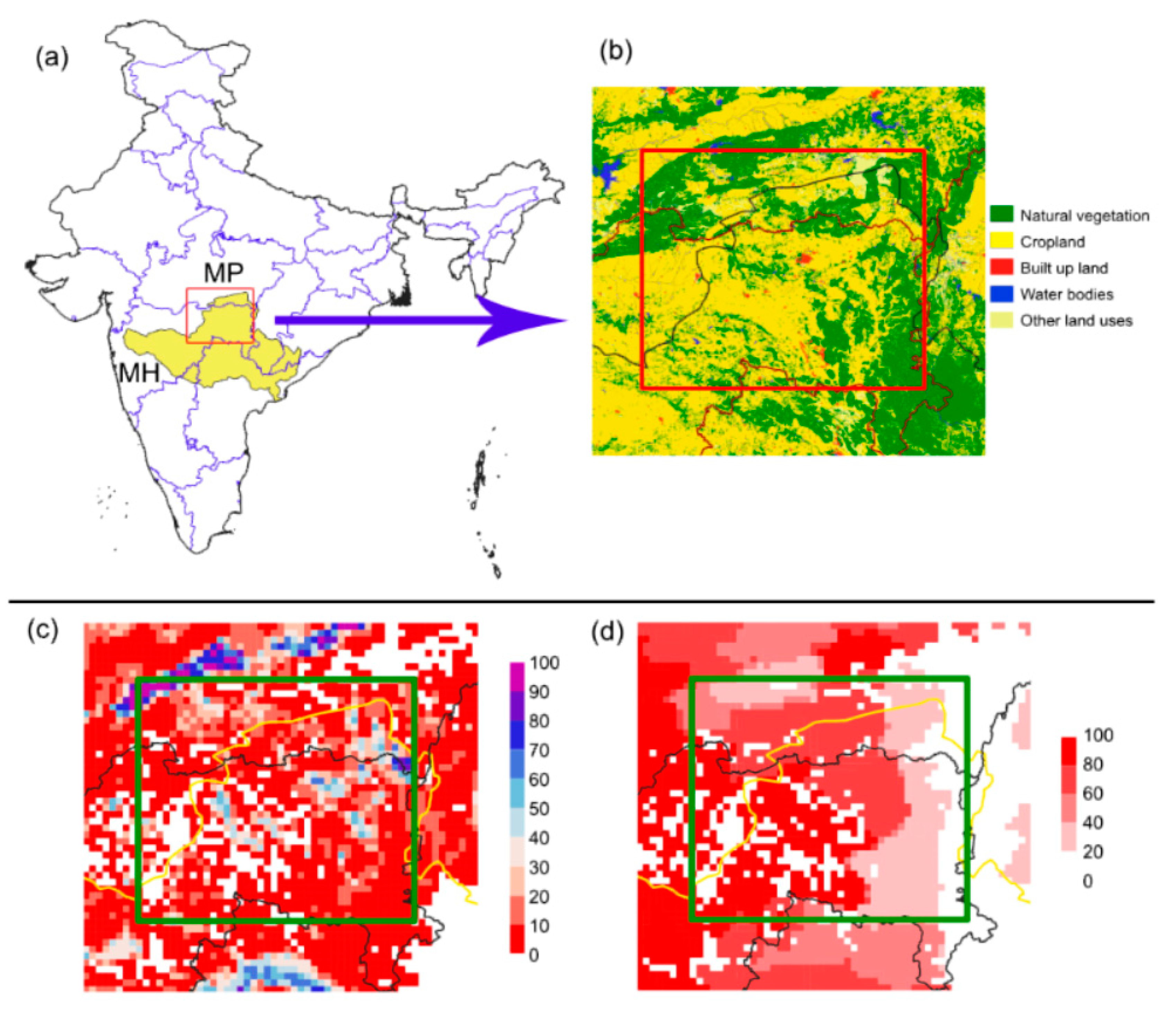
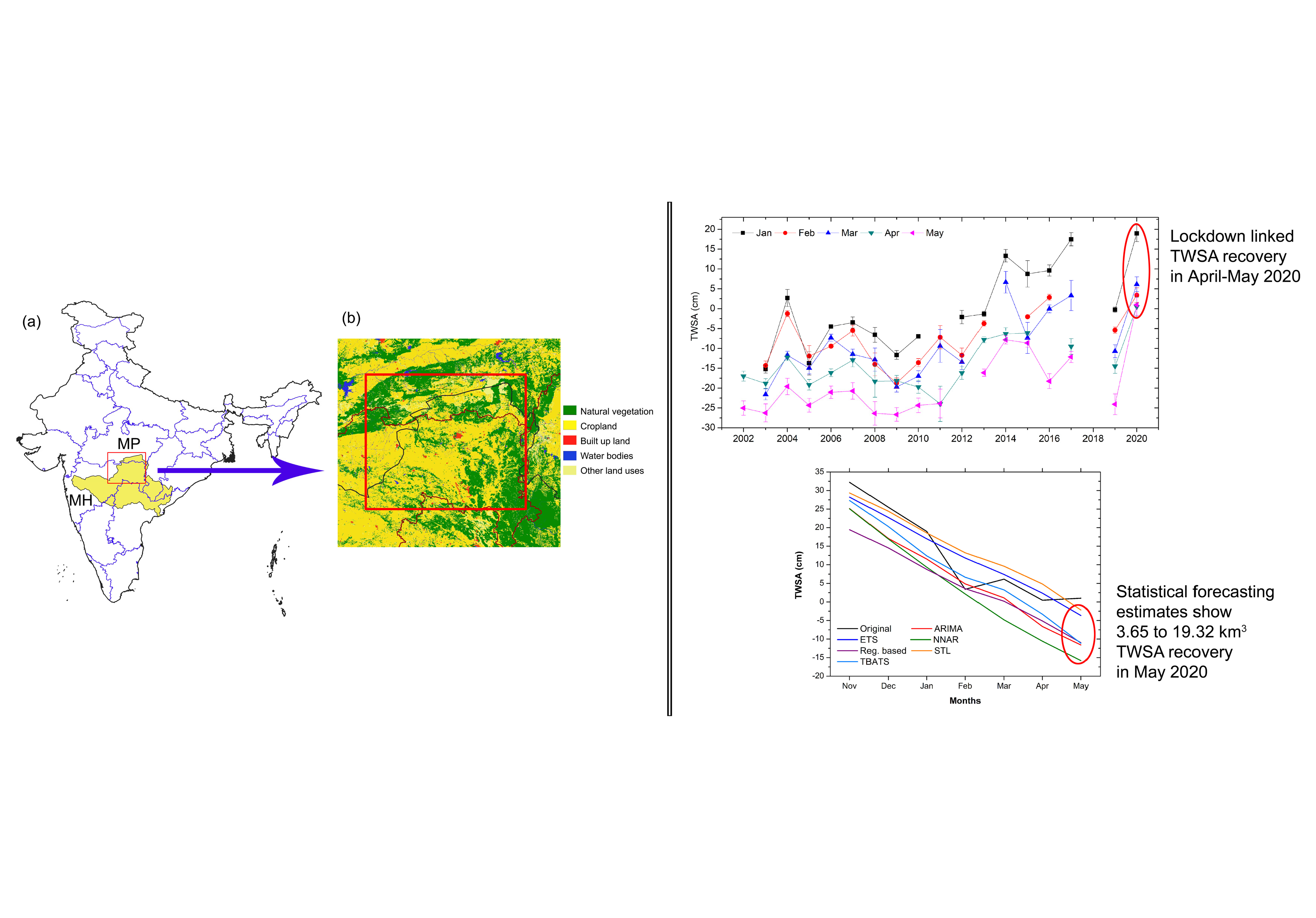
2.1. Study Area
2.2. GRACE TWSA
2.3. Precipitation and Evapotranspiration
2.4. Forecasting Techniques
2.5. Forecasting Performance Indicators
3. Results
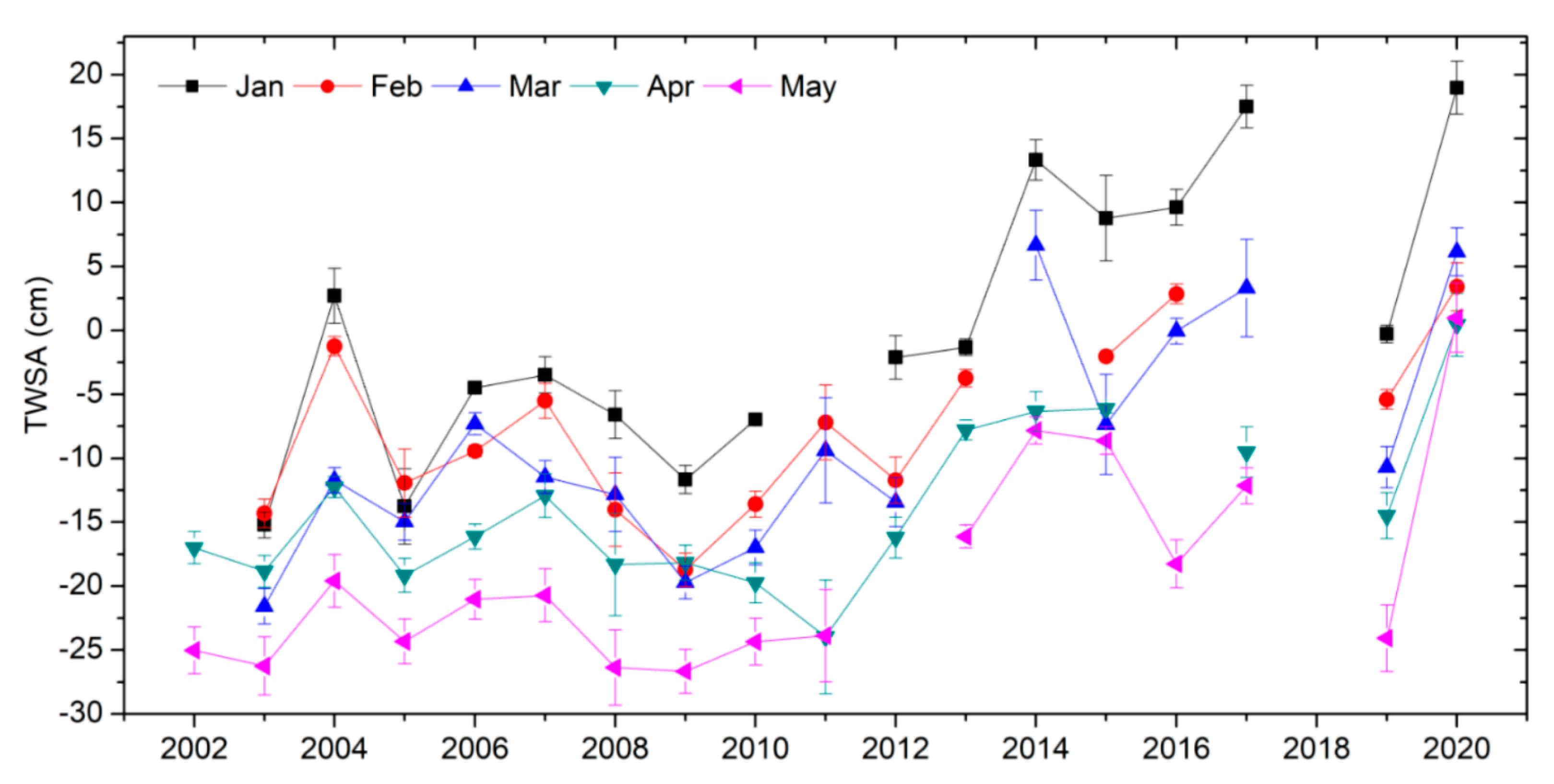
3.1. Precipitation and TWSA Patterns
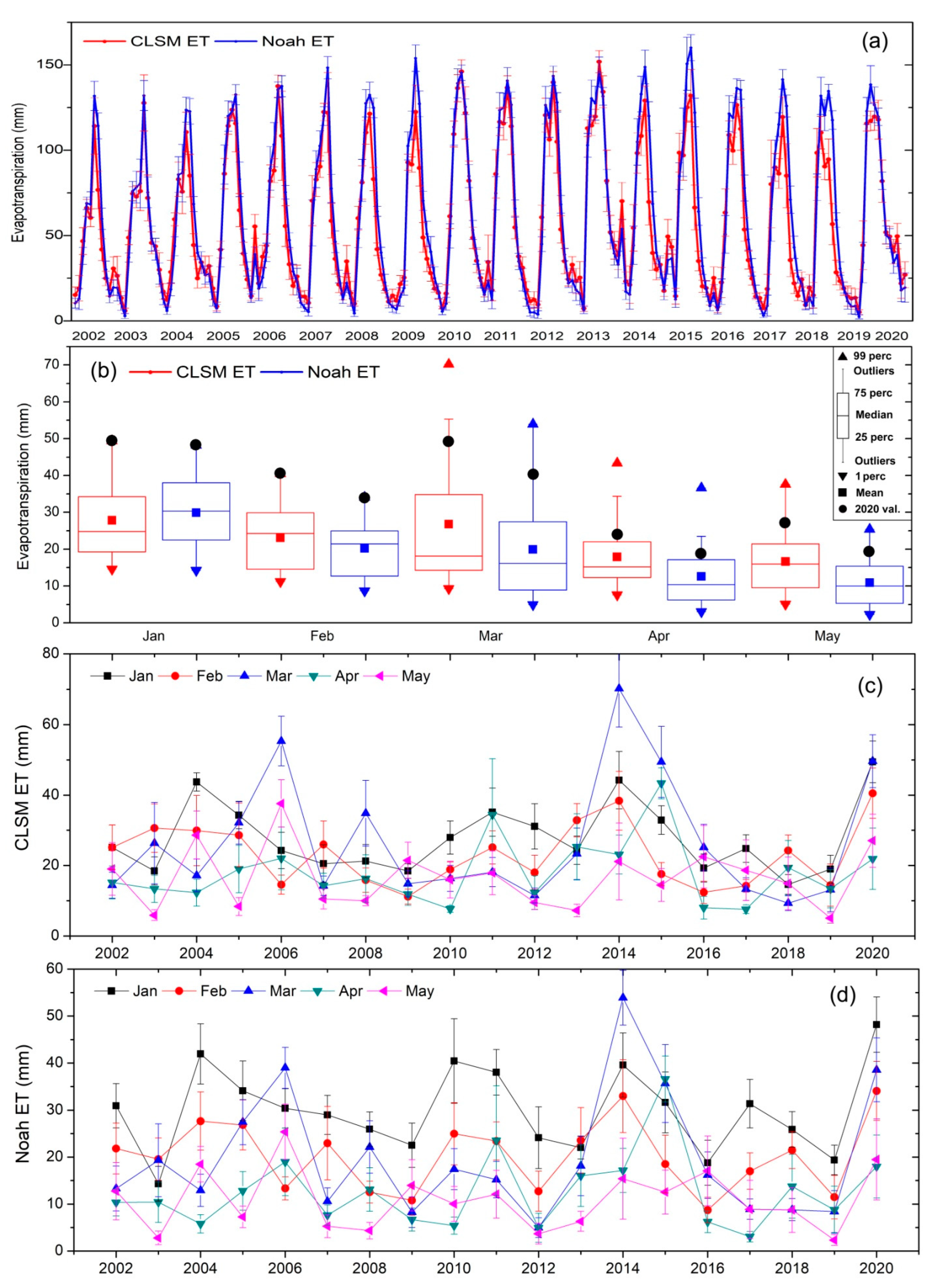
3.2. Evapotranspiration and TWSA Patterns
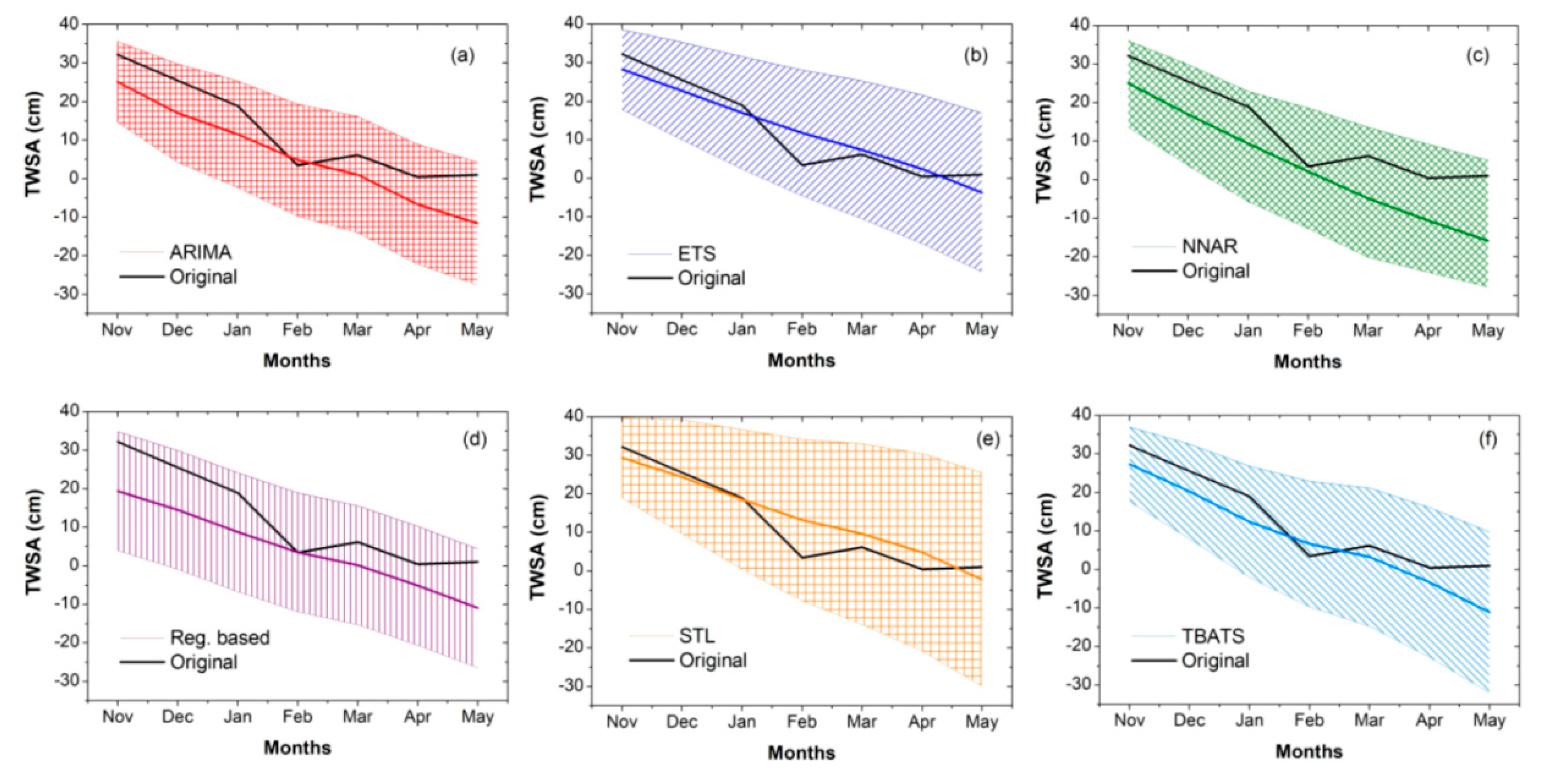
3.3. Statistical Forecasting of TWSA
4. Discussions
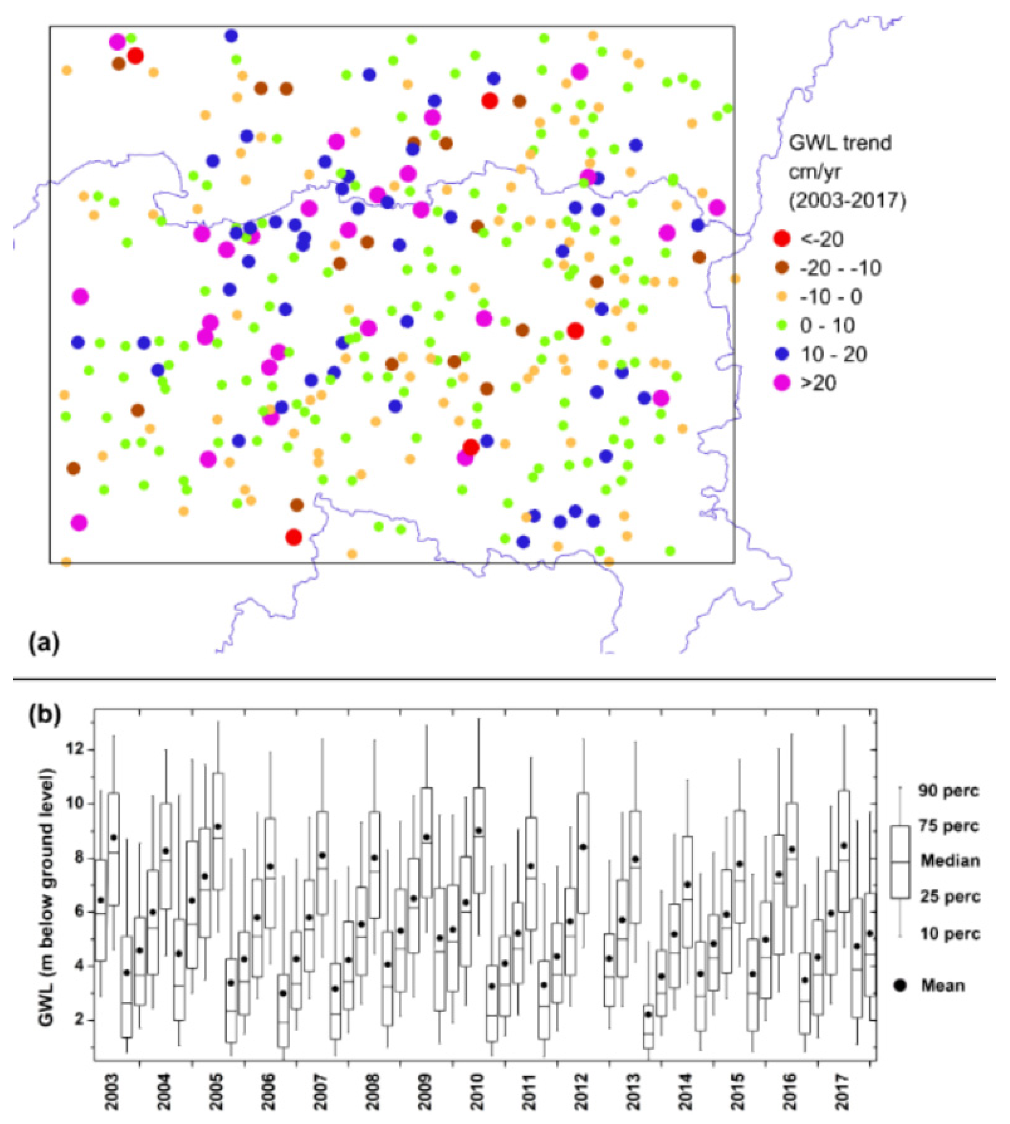
4.1. Influence of Policy Change on Long-Term TWSA Patterns
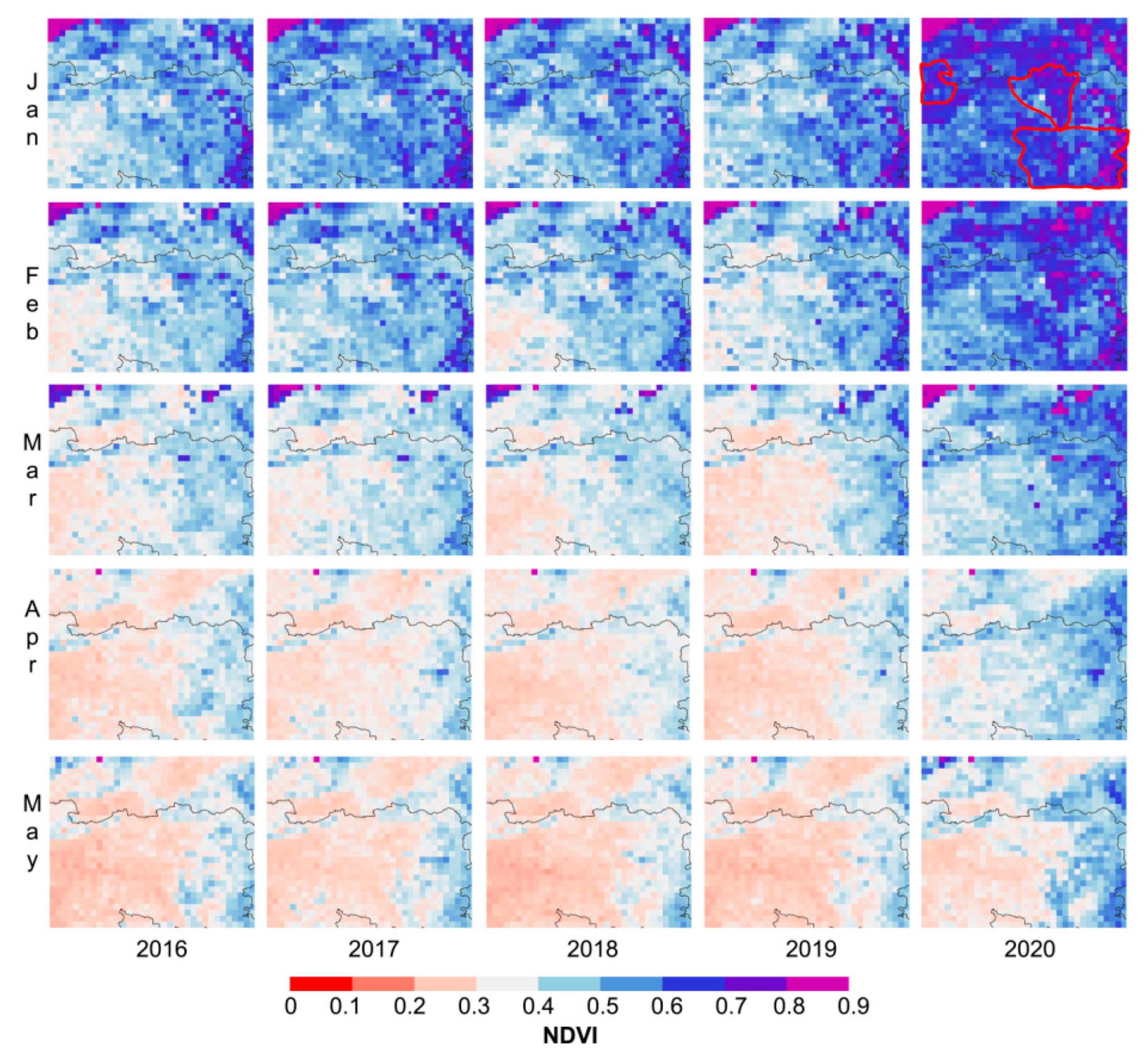
4.2. Change in Cropping Patterns
5. Conclusions
Supplementary Materials
Author Contributions
Funding
Data Availability Statement
Acknowledgments
Conflicts of Interest
References
- Bhanja, S.N.; Mukherjee, A.; Saha, D.; Velicogna, I.; Famiglietti, J.S. Validation of GRACE based groundwater storage anomaly using in-situ groundwater level measurements in India. J. Hydrol. 2016, 543, 729–738. [Google Scholar] [CrossRef]
- Rao, S.A.; Chaudhari, H.S.; Pokhrel, S.; Goswami, B.N. Unusual central Indian drought of summer monsoon 2008: Role of southern tropical Indian Ocean warming. J. Clim. 2010, 23, 5163–5174. [Google Scholar] [CrossRef]
- Venkateswarlu, B.; Raju, B.M.K.; Rao, K.V.; Rao, C.R. Revisiting drought-prone districts in India. Econ. Political Wkly. 2014, 49, 71–75. [Google Scholar]
- Verma, S.; Shah, M. Drought-Proofing through Groundwater Recharge: Lessons from Chief Ministers’ Initiatives in Four Indian States. World Bank Group. 2019. Available online: http://documents1.worldbank.org/curated/en/281991579881831723/pdf/Drought-Proofing-through-Groundwater-Recharge-Lessons-from-Chief-Ministers-Initiatives-in-Four-Indian-States.pdf (accessed on 19 September 2020).
- Behere, P.B.; Behere, A.P. Farmers’ suicide in Vidarbha region of Maharashtra state: A myth or reality? Indian J. Psychiatry 2008, 50, 124. [Google Scholar] [CrossRef] [PubMed]
- Dongre, A.R.; Deshmukh, P.R. Farmers’ suicides in the Vidarbha region of Maharashtra, India: A qualitative exploration of their causes. J. Inj. Violence Res. 2012, 4, 2. [Google Scholar] [CrossRef] [Green Version]
- National Crime Records Bureau (NCRB). Accidental Deaths & Suicides in India 2015, Table 2A.3. National Crime Records Bureau, Government of India. 2016. Available online: https://ncrb.gov.in/sites/default/files/adsi_reports_previous_year/table-2A.3.pdf (accessed on 15 September 2020).
- WHO. WHO Coronavirus (COVID-19) Dashboard. 2022. Available online: https://covid19.who.int/table (accessed on 25 February 2022).
- Ministry of Health and Family Welfare (MOHFW), 2022. COVID-19 Statewise Status. Ministry of Health and Family Welfare, Govt. of India. Available online: https://www.mohfw.gov.in/ (accessed on 26 February 2022).
- Box, G.E.; Jenkins, G.M. Time Series Analysis Forecasting and Control; Wisconsin University Madison Department of Statistics, Holden-Day: Madison, WI, USA, 1970; p. 553. [Google Scholar]
- Hodgson, F.D. The use of multiple linear regression in simulating ground-water level responses. Groundwater 1978, 16, 249–253. [Google Scholar] [CrossRef]
- Salas, J.D. Applied Modeling of Hydrologic Time Series; Water Resources Publication: Washington, DC, USA, 1980. [Google Scholar]
- Yaseen, Z.M.; El-Shafie, A.; Jaafar, O.; Afan, H.A.; Sayl, K.N. Artificial intelligence based models for stream-flow forecasting: 2000–2015. J. Hydrol. 2015, 530, 829–844. [Google Scholar] [CrossRef]
- Jain, S.K.; Das, A.; Srivastava, D.K. Application of ANN for reservoir inflow prediction and operation. J. Water Resour. Plan. Manag. 1999, 125, 263–271. [Google Scholar] [CrossRef]
- Daliakopoulos, I.N.; Coulibaly, P.; Tsanis, I.K. Groundwater level forecasting using artificial neural networks. J. Hydrol. 2005, 309, 229–240. [Google Scholar] [CrossRef]
- Shen, C.; Laloy, E.; Elshorbagy, A.; Albert, A.; Bales, J.; Chang, F.J.; Ganguly, S.; Hsu, K.L.; Kifer, D.; Fang, Z.; et al. HESS Opinions: Incubating deep-learning-powered hydrologic science advances as a community. Hydrol. Earth Syst. Sci. 2018, 22, 5639–5656. [Google Scholar] [CrossRef] [Green Version]
- Malakar, P.; Mukherjee, A.; Bhanja, S.N.; Sarkar, S.; Saha, D.; Ray, R.K. Deep learning-based forecasting of groundwater level trends in India: Implications for crop production and drinking water supply. ACS ES&T Eng. 2021, 1, 965–977. [Google Scholar]
- Nearing, G.S.; Kratzert, F.; Sampson, A.K.; Pelissier, C.S.; Klotz, D.; Frame, J.M.; Prieto, C.; Gupta, H.V. What role does hydrological science play in the age of machine learning? Water Resour. Res. 2021, 57, e2020WR028091. [Google Scholar] [CrossRef]
- Tapley, B.D.; Bettadpur, S.; Ries, J.C.; Thompson, P.F.; Watkins, M.M. GRACE measurements of mass variability in the Earth system. Science 2004, 305, 503–505. [Google Scholar] [CrossRef] [PubMed] [Green Version]
- Famiglietti, J.S.; Rodell, M. Water in the balance. Science 2013, 340, 1300–1301. [Google Scholar] [CrossRef]
- Rodell, M.; Famiglietti, J.S.; Wiese, D.N.; Reager, J.T.; Beaudoing, H.K.; Landerer, F.W.; Lo, M.H. Emerging trends in global freshwater availability. Nature 2018, 557, 651–659. [Google Scholar] [CrossRef]
- Wahr, J.M. Time-variable gravity from satellites. Treatise Geophys. 2007, 3, 213–237. [Google Scholar]
- Flechtner, F. AOD1B Product Description Document for Product Releases 1 to 4 (Rev. 3.1, 13 April 2007); GRACE Project Document; GeoForschungszentrum: Potsdam, Germany, 2007; p. 43. [Google Scholar]
- Roy, P.S.; Meiyappan, P.K.; Joshi, M.P.; Kale, V.K.; Srivastav, S.K.; Srivasatava, M.D.; Behera, A.; Roy, Y.; Sharma, R.M.; Ramachandran, P.; et al. Decadal Land Use and Land Cover Classifications across India, 1985, 1995, 2005; ORNL DAAC: Oak Ridge, TN, USA, 2016. [Google Scholar] [CrossRef]
- Siebert, S.; Henrich, V.; Frenken, K.; Burke, J. Global Map of Irrigation Areas Version 5; Rheinische Friedrich-Wilhelms-University: Bonn, Germany; Food, Agriculture Organization of the United Nations: Rome, Italy, 2013; Volume 2, pp. 1299–1327. [Google Scholar]
- Central Ground Water Board (CGWB). Aquifer Systems of India; G.o.I. Ministry of Water Resources: New Delhi, India, 2012; 92p.
- Saha, D.; Marwaha, S.; Mukherjee, A. Groundwater resources and sustainable management issues in India. In Clean and Sustainable Groundwater in India; Springer: Singapore, 2018; pp. 1–11. [Google Scholar]
- Bhanja, S.N.; Mukherjee, A.; Rodell, M.; Wada, Y.; Chattopadhyay, S.; Velicogna, I.; Pangaluru, K.; Famiglietti, J.S. Groundwater rejuvenation in parts of India influenced by water-policy change implementation. Sci. Rep. 2017, 7, 7453. [Google Scholar] [CrossRef] [Green Version]
- Watkins, M.M.; Wiese, D.N.; Yuan, D.-N.; Boening, C.; Landerer, F.W. Improved methods for observing Earth’s time variable mass distribution with GRACE using spherical cap mascons. J. Geophys. Res. Solid Earth 2015, 120, 2648–2671. [Google Scholar] [CrossRef]
- Wiese, D.N.; Landerer, F.W.; Watkins, M.M. Quantifying and reducing leakage errors in the JPL RL05M GRACE mascon solution. Water Resour. Res. 2016, 52, 7490–7502. [Google Scholar] [CrossRef]
- Wiese, N.D.; Yuan, D.-N.; Boening, C.; Landerer, F.W.; Watkins, M.M. JPL GRACE Mascon Ocean, Ice, and Hydrology Equivalent Water Height Release 06 Coastal Resolution Improvement (CRI) Filtered Version 1.0. PO. DAAC, CA, USA. 2018. Available online: https://podaac.jpl.nasa.gov/dataset/TELLUS_GRACE_MASCON_CRI_GRID_RL06_V1 (accessed on 25 July 2020). [CrossRef]
- Patel, P.M.; Saha, D.; Shah, T. Sustainability of groundwater through community-driven distributed recharge: An analysis of arguments for water scarce regions of semi-arid India. J. Hydrol. Reg. Stud. 2020, 29, 100680. [Google Scholar] [CrossRef]
- Cheng, M.; Tapley, B.D. Variations in the Earth’s oblateness during the past 28 years. J. Geophys. Res. 2004, 109, B09402. [Google Scholar] [CrossRef]
- Geruo, A; Wahr, J.; Zhong, S. Computations of the viscoelastic response of a 3-D compressible Earth to surface loading: An application to Glacial Isostatic Adjustment in Antarctica and Canada. Geophys. J. Int. 2013, 192, 557–572. [Google Scholar] [CrossRef]
- Funk, C.; Peterson, P.; Landsfeld, M.; Pedreros, D.; Verdin, J.; Shukla, S.; Husak, G.; Rowland, J.; Harrison, L.; Hoell, A.; et al. The climate hazards infrared precipitation with stations—A new environmental record for monitoring extremes. Sci. Data 2015, 2, 150066. [Google Scholar] [CrossRef] [Green Version]
- Prakash, S. Performance assessment of CHIRPS, MSWEP, SM2RAIN-CCI, and TMPA precipitation products across India. J. Hydrol. 2019, 571, 50–59. [Google Scholar] [CrossRef]
- Yoon, Y.; Kumar, S.V.; Forman, B.A.; Zaitchik, B.F.; Kwon, Y.; Qian, Y.; Rupper, S.; Maggioni, V.; Houser, P.; Kirschbaum, D.; et al. Evaluating the uncertainty of terrestrial water budget components over High Mountain Asia. Front. Earth Sci. 2019, 7, 120. [Google Scholar] [CrossRef] [Green Version]
- Rodell, M.; Houser, P.R.; Jambor, U.E.A.; Gottschalck, J.; Mitchell, K.; Meng, C.J.; Arsenault, K.; Cosgrove, B.; Radakovich, J.; Bosilovich, M.; et al. The global land data assimilation system. Bull. Am. Meteorol. Soc. 2004, 85, 381–394. [Google Scholar] [CrossRef] [Green Version]
- Li, X.; Long, D.; Han, Z.; Scanlon, B.R.; Sun, Z.; Han, P.; Hou, A. Evapotranspiration estimation for Tibetan plateau headwaters using conjoint terrestrial and atmospheric water balances and multisource remote sensing. Water Resour. Res. 2019, 55, 8608–8630. [Google Scholar] [CrossRef]
- Ma, N.; Szilagyi, J. The CR of evaporation: A calibration-free diagnostic and benchmarking tool for large-scale terrestrial evapotranspiration modeling. Water Resour. Res. 2019, 55, 7246–7274. [Google Scholar] [CrossRef] [Green Version]
- Pascolini-Campbell, M.A.; Reager, J.T.; Fisher, J.B. GRACE-based mass conservation as a validation target for basin-scale evapotranspiration in the contiguous United States. Water Resour. Res. 2020, 56, e2019WR026594. [Google Scholar] [CrossRef]
- Contreras, J.; Espinola, R.; Nogales, F.J.; Conejo, A.J. ARIMA models to predict next-day electricity prices. IEEE Trans. Power Syst. 2003, 18, 1014–1020. [Google Scholar] [CrossRef]
- Zhang, G.P. Time series forecasting using a hybrid ARIMA and neural network model. Neurocomputing 2003, 50, 159–175. [Google Scholar] [CrossRef]
- Hyndman, R.J.; Athanasopoulos, G. Forecasting: Principles and Practice; OTexts: Heathmont, Australia, 2018. [Google Scholar]
- Brown, R.G. Statistical Forecasting for Inventory Control; McGraw/Hill: New York, NY, USA, 1959. [Google Scholar]
- Holt, C.C. Planning Production, Inventories, and Work Force; Prentice-Hall: Englewood Cliff, NJ, USA, 1960; Chapter 14. [Google Scholar]
- Brown, R.G. Smoothing, Forecasting and Prediction of Discrete Time Series; Prentice-Hall: Englewood Cliff, NJ, USA, 1963. [Google Scholar]
- Gardner, E.S., Jr. Exponential smoothing: The state of the art. J. Forecast. 1985, 4, 1–28. [Google Scholar] [CrossRef]
- Gardner, E.S., Jr. Exponential smoothing: The state of the art—Part II. Int. J. Forecast. 2006, 22, 637–666. [Google Scholar] [CrossRef]
- Cleveland, R.B.; Cleveland, W.S.; McRae, J.E.; Terpenning, I. STL: A seasonal-trend decomposition. J. Off. Stat. 1990, 6, 3–73. [Google Scholar]
- De Livera, A.M.; Hyndman, R.J.; Snyder, R.D. Forecasting time series with complex seasonal patterns using exponential smoothing. J. Am. Stat. Assoc. 2011, 106, 1513–1527. [Google Scholar] [CrossRef] [Green Version]
- Moriasi, D.N.; Arnold, J.G.; van Liew, M.W.; Bingner, R.L.; Harmel, R.D.; Veith, T.L. Model evaluation guidelines for systematic quantification of accuracy in watershed simulations. Trans. ASABE 2007, 50, 885–900. [Google Scholar] [CrossRef]
- Nash, J.E.; Sutcliffe, J.V. River flow forecasting through conceptual models part I—A discussion of principles. J. Hydrol. 1970, 10, 282–290. [Google Scholar] [CrossRef]
- Gupta, H.V.; Sorooshian, S.; Yapo, P.O. Status of automatic calibration for hydrologic models: Comparison with multilevel expert calibration. J. Hydrol. Eng. 1999, 4, 135–143. [Google Scholar] [CrossRef]
- Helsel, D.R.; Hirsch, R.M. Statistical Methods in Water Resources; Elsevier: Amsterdam, The Netherlands, 1992; p. 49. [Google Scholar]
- Hodrick, R.J.; Prescott, E.C. Postwar US business cycles: An empirical investigation. J. Money Credit. Bank 1997, 29, 1–16. [Google Scholar] [CrossRef]
- Ravn, M.O.; Uhlig, H. On adjusting the Hodrick-Prescott filter for the frequency of observations. Rev. Econ. Stat. 2002, 84, 371–376. [Google Scholar] [CrossRef] [Green Version]
- Department of Agriculture and Cooperation (DAC). Vidarbha Intensive Irrigation Development Programme (VIIDP); Ministry of Agriculture, Government of India: New Delhi, India, 2012; p. 8. Available online: http://agricoop.nic.in/sites/default/files/VIIDP.pdf (accessed on 10 September 2020).
- Law and Judiciary Department (LJD). The Maharashtra Management of Irrigation Systems by Farmers act 2005; Law and Judiciary Department, Government of Maharashtra: Mumbai, Maharashtra. Available online: https://lj.maharashtra.gov.in/Site/Upload/Acts/5-The%20Maha.Mment%20of%20Irri.Sys.byFarmer%20Act-2005.pdf (accessed on 19 September 2020).
- World Bank. Maharashtra Project on Climate Resilient Agriculture; World Bank Group: Washington, DC, USA, 2018; Available online: https://documents.worldbank.org/en/publication/documents-reports/documentdetail/704731519959668277/india-maharashtra-project-on-climate-resilient-agriculture-project (accessed on 25 September 2020).
- Central Water Commission (CWC). National Register of Large Dams–2018; Central Water Commission: New Delhi, India, 2018; p. 224. Available online: http://cwc.gov.in/national-register-large-dams (accessed on 23 September 2020).
- Central Ground Water Board (CGWB). Master Plan for Artificial Recharge to Ground Water in India; G.o.I. Ministry of Water Resources: New Delhi, India, 2013; 225p.
- Bhusari, V.; Katpatal, Y.B.; Kundal, P. An innovative artificial recharge system to enhance groundwater storage in basaltic terrain: Example from Maharashtra, India. Hydrogeol. J. 2016, 24, 1273–1286. [Google Scholar] [CrossRef]
- Frappart, F.; Ramillien, G.; Ronchail, J. Changes in terrestrial water storage versus rainfall and discharges in the Amazon basin. Int. J. Climatol. 2013, 33, 3029–3046. [Google Scholar] [CrossRef] [Green Version]
- Prakash, S.; Gairola, R.M.; Papa, F.; Mitra, A.K. An assessment of terrestrial water storage, rainfall and river discharge over Northern India from satellite data. Curr. Sci. 2014, 107, 1582–1586. [Google Scholar]
- Didan, K. MOD13C2 MODIS/Terra Vegetation Indices Monthly L3 Global 0.05Deg CMG V006 [Data Set]. NASA EOSDIS Land Processes DAAC. 2015. Available online: https://doi.org/10.5067/MODIS/MOD13C2.006 (accessed on 25 July 2020).
- United States Geological Survey (USGS). NDVI, the Foundation for Remote Sensing Phenology. 2020. Available online: https://www.usgs.gov/core-science-systems/eros/phenology/science/ndvi-foundation-remote-sensing-phenology?qt-science_center_objects=0#qt-science_center_objects (accessed on 22 September 2020).
- Bhanja, S.N.; Malakar, P.; Mukherjee, A.; Rodell, M.; Mitra, P.; Sarkar, S. Using satellite-based vegetation cover as indicator of groundwater storage in natural vegetation areas. Geophys. Res. Lett. 2019, 46, 8082–8092. [Google Scholar] [CrossRef]
- Vittal, K.P.R.; Sinha, P.K.; Chary, G.R.; Sankar, G.M.; Srijaya, T.; Ramakrishna, Y.S.; Samra, J.S.; Singh, G. Districtwise promising technologies for rainfed rice based production system in India. In All India Co-ordinated Research Project for Dryland Agriculture; Central Research Institute for Dryland Agriculture, Indian Council of Agricultural Research: Hyderabad, India, 2004; Volume 500, p. 59. [Google Scholar]
- Dalezios, N.R.; Domenikiotis, C.; Loukas, A.; Tzortzios, S.T.; Kalaitzidis, C. Cotton yield estimation based on NOAA/AVHRR produced NDVI. Phys. Chem. Earth Part B Hydrol. Ocean. Atmos. 2001, 26, 247–251. [Google Scholar] [CrossRef]
- Tan, C.W.; Zhang, P.P.; Zhou, X.X.; Wang, Z.X.; Xu, Z.Q.; Mao, W.; Li, W.X.; Huo, Z.Y.; Guo, W.S.; Yun, F. Quantitative monitoring of leaf area index in wheat of different plant types by integrating NDVI and Beer-Lambert law. Sci. Rep. 2020, 10, 929. [Google Scholar] [CrossRef]
- Agropedia. Cultivation of Wheat. Indian Institute of Technology Kanpur. 2020. Available online: http://agropedia.iitk.ac.in/content/cultivation-wheat (accessed on 21 September 2020).
- Parthasarathy, B.; Sontakke, N.A.; Monot, A.A.; Kothawale, D.R. Droughts/floods in the summer monsoon season over different meteorological subdivisions of India for the period 1871–1984. J. Climatol. 1987, 7, 57–70. [Google Scholar] [CrossRef]
- Pai, D.S.; Sridhar, L.; Guhathakurta, P.; Hatwar, H.R. District-wide drought climatology of the southwest monsoon season over India based on standardized precipitation index (SPI). Nat. Hazards 2011, 59, 1797–1813. [Google Scholar] [CrossRef]
- Guhathakurta, P.; Menon, P.; Inkane, P.M.; Krishnan, U.; Sable, S.T. Trends and variability of meteorological drought over the districts of India using standardized precipitation index. J. Earth Syst. Sci. 2017, 126, 120. [Google Scholar] [CrossRef] [Green Version]


| ARIMA | ETS | NNAR | Regression Based | STL | TBATS | |
|---|---|---|---|---|---|---|
| NSE | 0.59 | 0.87 | 0.26 | 0.40 | 0.85 | 0.73 |
| PBIAS % | 52.66 | 2.03 | 74.54 | 65.28 | −11.58 | 36.75 |
| RSR | 0.59 | 0.33 | 0.80 | 0.72 | 0.36 | 0.49 |
| RMSE | 7.67 | 4.24 | 10.30 | 9.23 | 4.59 | 6.27 |
| MAE | 7.01 | 3.57 | 9.34 | 8.23 | 3.60 | 5.54 |
| R | 0.95 | 0.94 | 0.95 | 0.94 | 0.93 | 0.94 |
Publisher’s Note: MDPI stays neutral with regard to jurisdictional claims in published maps and institutional affiliations. |
© 2022 by the authors. Licensee MDPI, Basel, Switzerland. This article is an open access article distributed under the terms and conditions of the Creative Commons Attribution (CC BY) license (https://creativecommons.org/licenses/by/4.0/).
Share and Cite
Bhanja, S.N.; Sekhar, M. Short-Term and Long-Term Replenishment of Water Storage Influenced by Lockdown and Policy Measures in Drought-Prone Regions of Central India. Remote Sens. 2022, 14, 1768. https://doi.org/10.3390/rs14081768
Bhanja SN, Sekhar M. Short-Term and Long-Term Replenishment of Water Storage Influenced by Lockdown and Policy Measures in Drought-Prone Regions of Central India. Remote Sensing. 2022; 14(8):1768. https://doi.org/10.3390/rs14081768
Chicago/Turabian StyleBhanja, Soumendra N., and M. Sekhar. 2022. "Short-Term and Long-Term Replenishment of Water Storage Influenced by Lockdown and Policy Measures in Drought-Prone Regions of Central India" Remote Sensing 14, no. 8: 1768. https://doi.org/10.3390/rs14081768
APA StyleBhanja, S. N., & Sekhar, M. (2022). Short-Term and Long-Term Replenishment of Water Storage Influenced by Lockdown and Policy Measures in Drought-Prone Regions of Central India. Remote Sensing, 14(8), 1768. https://doi.org/10.3390/rs14081768