2.1. Ground Penetrating Radar and the Similarity to Medical 3D Image Data
High-resolution 3D GPR datasets for archaeological prospection are computed from the echoes of an electromagnetic pulse emitted into the ground by a transmitting antenna and recorded using a receiving antenna. Practical survey grids are in the order of sub decimeter intervals, depending on the radar wavelength used [
7,
13]. The properties of the recorded echo wave strongly depend on the physical properties of the archaeological features, as well as the physical properties such as composition, grain size, pore volume, humidity of the surrounding soil matrix, or embedded archaeological and geological deposits. GPR dataset reconstruction aims at the computation of the radar reflectivity at distinct 3D locations beneath the recording surface. The necessary transformation of the signal recorded in 2D space to the 3D volume is typically calculated based on estimated signal propagation velocities; however, the complex radar wave/soil interaction requires extensive pre-processing, including band-pass filtering and migration to avoid artifacts such as excessive noise and reflector localization ambiguities. Finally, the commonly used reflectivity measure is computed from the absolute amplitude of the adjusted wave signal, resampled at each cell or voxel of the dataset grid defined over the measurement volume (3D cuboid) [
21,
27].
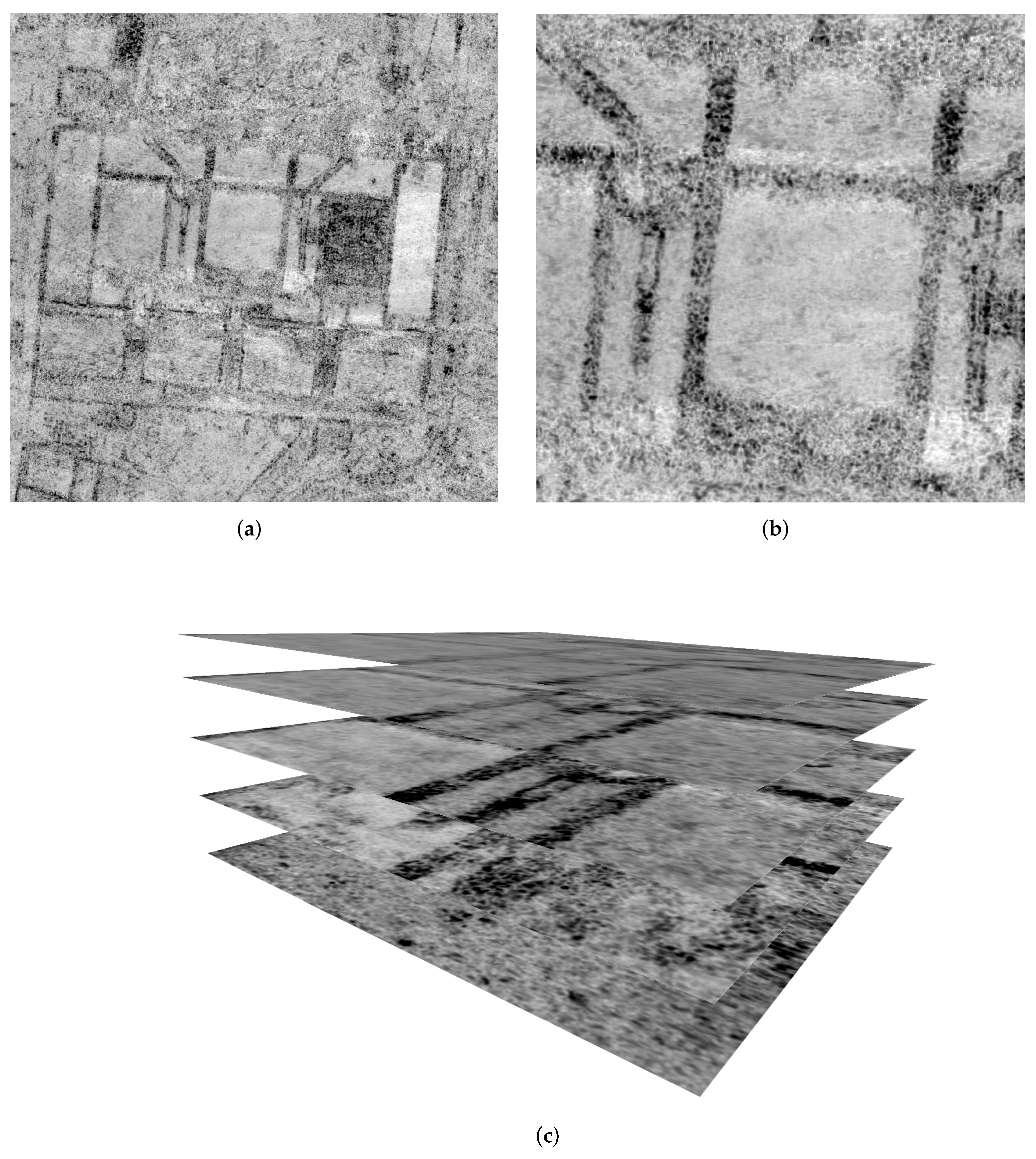
In the archaeological interpretation process, GPR datasets are generally visualized as stacks of 2D time or depth slice images, which are horizontal sections through the dataset volume representing a certain depth or time interval (see
Figure 1c). In addition, vertical sections can be extracted and explored in orthogonal views for enhanced perception of 3D structures. For display, we deliberately use a grey scale ranging from white for low radar reflectivity to black for high radar reflectivity (see
Figure 1).
Larger time- or depth-intervals reduce the total number of stacked images to be analyzed and, at the same time, the amount of noise. The aggregation of values along the vertical time/depth axis supports the detectability of linear or geometrical outlines of structures such as walls within a noisy background, etc.; however, it inevitably results in a loss of contour fidelity when it comes to the definition of a specific feature during the interpretative mapping. In addition, the technique to display the stack of GPR data slices with minimal depth or time intervals, in the order of half of the wavelength, as an infinite video loop was established as a visualization standard [
28]. This approach seems to support the interpreter in the initial formation of a mental three-dimensional model of the stratification under investigation. The spatial relationships of the features and structures recorded in the radar survey become more readily comprehensible through animation, as the information that is only fragmentarily mapped in the individual slices is merged through the motion, and thus becomes easier to comprehend [
29].
It is also appropriate to use varying parameters for the generation of the time and depth slices, as well as to use different processing methods such as GPR attributes [
30]. Amplitude maps can be complemented with sectional views for improved three-dimensional perception. This is especially useful for surveys with high geological complexity. Integrating additional data or modalities can improve comprehension of GPR datasets and facilitate their interpretation [
31].
For the implementation of the interpretation process, GIS environments with the appropriate tools are frequently employed. GIS environments do not only support GPR dataset visualization in the form of horizontal 2D slices with globally referenced positioning, but also provide the functionality to overlay supporting 2D images and 2.5D data derived from magnetometry, remote sensing, and existing geographical or historical maps. Software solutions such as
GPR-Slice and
GPR-Insights (
https://www.screeningeagle.com/en/products/category/software/gpr-slice-insights#GPR-Insights, accessed on 29 January 2022) offer comparable functionality, but also offer GPR data processing, visualization of 2D time or depth slices and profiles, as well as the extraction of 3D iso-surfaces from the GPR datasets to be combined with additional 2D images and 3D models. The support for integrating 3D models in GIS is improving but still limited. Basic support for the visualization of 3D volume datasets such as GPR has only recently been introduced in widespread GIS environments such as
ArcGIS (version 2.6 and higher) (
https://pro.arcgis.com/de/pro-app/latest/help/mapping/layer-properties/what-is-a-voxel-layer-.htm, accessed on 29 January 2022). More general volume visualization tools such as
Voxler (
https://www.goldensoftware.com/products/voxler, accessed on 29 January 2022) or
VG Studio Max (
https://www.volumegraphics.com/de/produkte/vgstudio-max.html, accessed on 29 January 2022) support multiple volume datasets, as well as the inclusion of non-volumetric data. Still, their flexibility is limited in terms of the targeted local control of the visualization outcome, as well as for the integration of non-volumetric data as required for the archaeological interpretation process.
The 3D visualization of GPR datasets in the form of iso-surfaces was established at an early stage [
32] and is still widely used [
33,
34], e.g., to depict Roman foundations and walls. Iso-surfaces provide acceptable but clearly suboptimal results for the archaeological analysis, since they assume that relevant structures can be separated on the basis of different dataset values.
In GPR data this is not the case due to high intensity variations and intrinsic noise throughout the datasets. Relevant structures in extracted iso-surfaces either appear fragmented or are not visible at all, depending on the choice of the iso value. Generally, iso-surfaces sacrifice most of the data immanent information for just a single value transition surface.
The techniques presented in [
35] represent an early example of the application of so-called direct volume rendering (DVR) techniques to GPR datasets, which generally compute 3D views from volumetric data taking into account all dataset information available. Although focusing on the integration of GPR and EM-61 data into one single 3D volume, work in [
35] already emphasized the importance of 3D visualization for object localization and the interpretation process and the key role of the appropriate transfer function mapping measurement values to optical properties. Unfortunately, it had no further impact on archaeological applications. Consequently, 3D volume visualization techniques are not yet established as a standard for archaeological GPR applications. Other application examples of DVR in the geoscience context exist, but are rare, e.g., the visualization of volumetric atmospheric data as part of large multi-variate datasets [
36,
37].
Medical imaging techniques such as X-ray computed tomography (CT) or magnetic resonance imaging (MRI) provide 3D volume datasets similar to GPR. The 2D visualization tools used in medical imaging such as
ITK-Snap (
http://www.itksnap.org, accessed on 29 January 2022) or
3D Slicer (
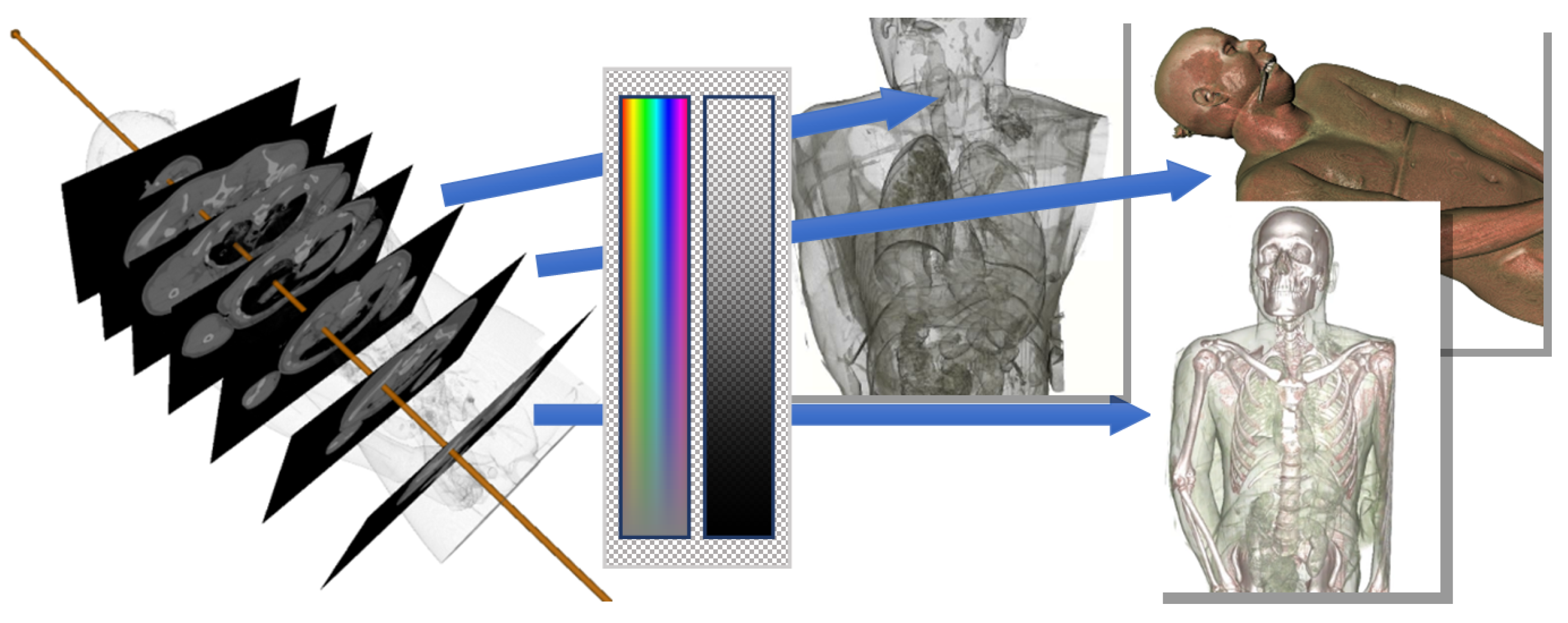
https://www.slicer.org/, accessed on 29 January 2022) use coupled cross-sectional views as their central visualization means. This approach has become established as a standard in medical imaging, since it simplifies tracing the course of structures in 3D space compared to a single view. The cross-sections displayed are not limited to the dataset grid axes. Instead, they are obtained by sampling the dataset on arbitrarily oriented slice planes. This may also include the aggregation of sample values in a slab region around the slice plane using operations such as averaging, minimum, or maximum. Many clinical questions do not require the full dataset resolution by modern CT scanners. In these cases, the loss of detail information due to the aggregation is acceptable and outweighed by the time saved due to the reduced number of slices to be processed. The 3D visualization of CT data using iso-surface rendering is well-suited to depict structures well-defined by ideally unique dataset value ranges, such as bones; however, iso-surfaces have been largely replaced by DVR using a transfer function mapping dataset values to color and transparency. This approach is more flexible, supporting semi-transparent representations as well as the visual separation of multiple features, as far as they are characterized by unambiguous dataset value ranges. DVR images are typically computed by casting view rays through the dataset volume, densely sampling the data, applying the transfer function, computing artificial lighting at data-immanent feature surfaces, and finally the accumulation of the visual contribution of all samples to a color value as shown in
Figure 2 [
38].
Although the visualization functionality offered by medical tools is useful for the archaeological analysis of GPR data, their applicability in archaeology is limited. Medical software tools are not developed with an archaeological workflow in mind, nor designed to support the interpretative mapping. Consequently, the support for the integration of multiple volume datasets as well as georeferencing is missing. Furthermore, the unmodified use of medical DVR has been found to be insufficient for depicting archaeological features in the interpretation process as well as for illustration purposes [
39,
40]. Compared to their medical counterparts, GPR datasets show a different value distribution and characteristics. While CT Hounsfield values are characteristic for particular tissue types, with moderate variations, GPR data may show high frequency intensity changes over the entire dataset volume, e.g., in stony ground, which leads to noisy looking images. Noise may also be introduced in the measurement and reconstruction stage, due to limited methods and a priori knowledge on the volume under investigation. Soil moisture reduces the contrast. These are challenging problems, which indicate the need for the development of specific data pre-processing workflows. Nevertheless, visualization methods for medical data offer numerous inspirations for archaeological applications but require a special adaptation to the requirements and the objectives, i.e., optimal visibility of archaeological structures for their identification and definition in the interpretative process.
2.2. Integrated 3D Visualization for Archaeological Prospection Data
Based on the demand for 3D visualization of prospection data and standards developed in medical imaging, we specified a novel integrated visualization approach for archaeological 3D prospection datasets, with the goal to optimally support the GPR dataset exploration as well as the interpretation process. The application of specific 3D image processing techniques is crucial to improve the dataset suitability for 3D visualization, and thereby to achieve a representation quality that allows a novel, interactive computer-assisted 3D interpretation process. It is also required to be able to seamlessly incorporate 2D images for multimodal analysis, since this can potentially contribute valuable information. Magnetometry images, for example, depict metal finds or former fireplaces, and may thereby provide valuable clues to the past use of particular buildings or rooms. Airborne images and laser scans provide context information. Integration of still standing monuments above the surface in the form of 3D point clouds from terrestrial laser scanning or 3D meshes from image-based modeling or virtual reconstruction models contributes more context information. The combined 3D visualization of heterogeneous data supports the development of a deep understanding of the initial GPR dataset, as well as the whole area under investigation through the explicit integration of the multimodal information measured by the various sensors.
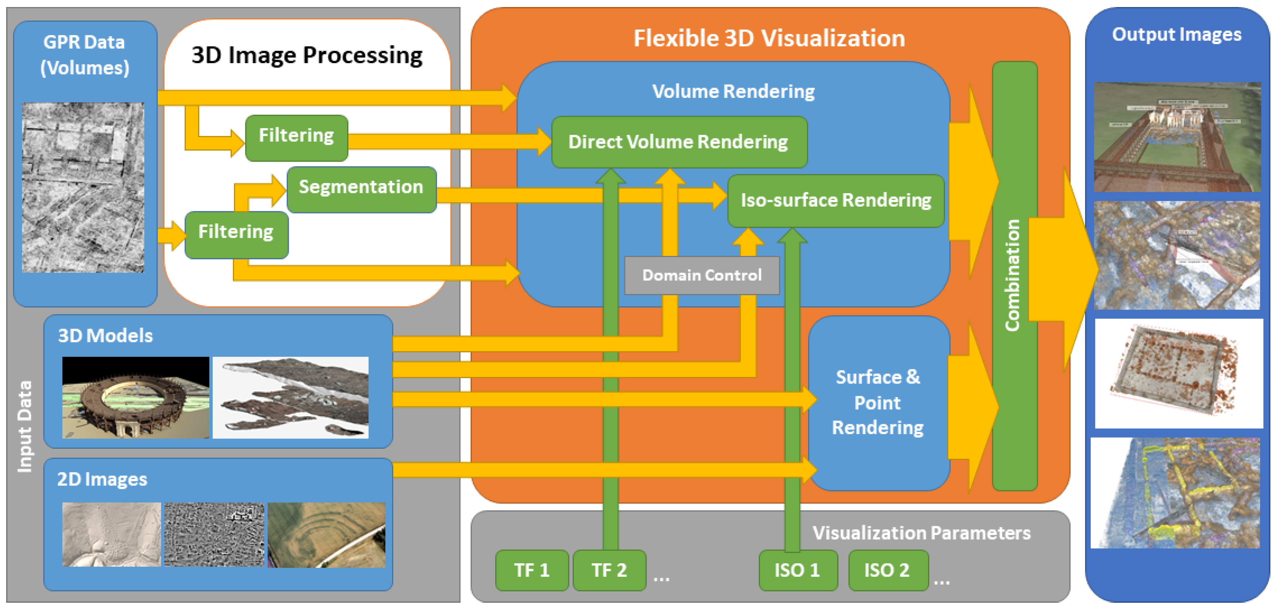
Figure 3 gives an overview of the proposed 3D visualization system for heterogeneous archaeological prospection data centered around a flexible 3D visualization algorithm capable of handling the respective data types. GPR datasets may first undergo 3D image processing using a variety of filters (
Section 2.3.1) and segmentation algorithms (
Section 2.4). Original and derived 3D volumes are visualized using DVR or iso-surface rendering using transfer functions or iso values, respectively (
Section 2.3.2). The 3D models, point clouds, and 2D images are first handled using a standard rendering pipeline, and later seamlessly integrated with the volume rendering contributions leading to the output image (
Section 2.5). The 3D surface models may also be used to define the visible portion of volume datasets as well as application domains of the transfer function, which offers a multitude of possibilities for visualization (
Section 2.6) and interpretation (
Section 3.1).
2.3. GPR Data Pre-Processing for 3D Visualization
Direct application of volume rendering techniques, such as DVR or iso-surface rendering for GPR data, is basically possible; however, the results do not reach the quality of DVR in the medical approach. This is due to the different dataset properties related to the measurement principle, the underlying physics, and the reconstruction process. A detailed comparison would go far beyond the scope of this work. Put in a nutshell, CT measures the X-ray permeability, which is different for air, soft tissue, and bones with moderate variations within their structure. Structures of interest such as organs or lesions are often an order of magnitude (centimeters) larger than the dataset resolution (approx. 0.5 mm). Finally, there is a high degree of redundancy in the measurement process, which, combined with state-of-the-art reconstruction algorithms, leads to crisp datasets with a low number of artifacts.
In GPR imaging there is a trade-off between the achievable depth of penetration and the possible spatial resolution, both linked to the applied radar wavelength [
7,
21]. We often use 400 or 500 MHz antennas, leading to a penetration depth of approximately 2 to 3 m, defining the vertical extent of the measurement volume. The spatial resolutions of the reconstructed 3D data volume typically lie in the range of 25 cm up to 2 cm, which corresponds to the extent of the smallest archaeological features of interest such as individual walls, basements for columns, postholes, or hypocaust pillars. Nevertheless, such features are only covered by a small number of voxels even in high-resolution GPR datasets.
A trained human interpreter can perceive the outlines of buildings, depict different types of floors, open squares, garden areas, etc., based on the visual inspection of 2D GPR slices (see
Figure 1). This is to a large extent due to the ability of the human brain to supplement incomplete data with existing a priori knowledge through analogy inferences in the mental interpretation process. This way a human expert may recognize contextual information that is not derivable for an automatic segmentation or classification system; thus, the human interpreter uses a type of mental filtering that reduces the complex data visualizations to the archaeologically relevant content by depicting geometrical layouts, individual features, or by differentiating various patterns in relation to the complete image content. Noise normally does not affect this ability, as it is faded out in the mental interpretation process.
In the proposed approach the interpretative process is facilitated using 3D volume visualizations based on DVR offering the interpreter a comprehensive and thus enhanced perception of the data in 3D space. DVR reveals the 3D shapes of major structures of archaeological interest such as walls, but the images produced appear noisy (see
Figure 4). It is possible to identify archaeologically relevant information such as walls, floors, hypocausts, ditches, or pits within the displayed diffuse GPR patterns. The exact delineation of individual features or larger structures in the course of the interpretative mapping is challenging in both 2D and 3D visualizations. Small features can easily be mistaken for ground structures.
2.3.1. Filtering of GPR Data Volumes for 3D Visualization
We investigated image processing techniques capable of improving the suitability of GPR datasets for 3D visualization techniques in the sense of 3D illustrations easier to understand. Such processing techniques should produce datasets with increased perceptibility of archaeologically relevant features and their respective 3D shapes, as well as a better distinguishability from geological structures in order to facilitate the interpretative process.
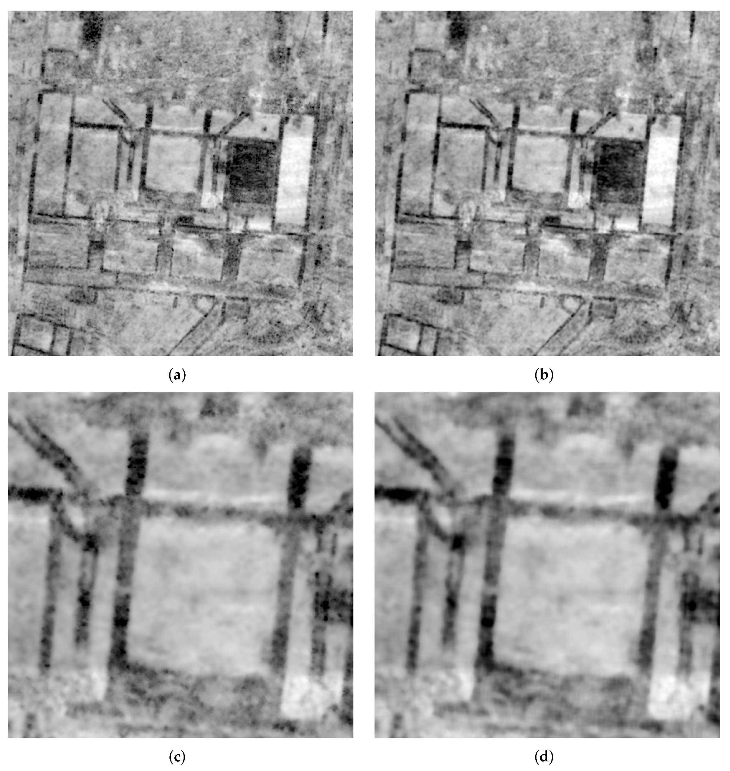
Image smoothing filters such as
averaging and
Gaussian smoothing remove noise and thereby inherently lead to more homogeneous GPR images. The improvement of such filters comes at the cost of blurred contours; therefore, we investigated the matter of edge-preserving image smoothing filters often used for medical tomography data and their applicability for the enhancement of GPR datasets. The simplest form of smoothing filters attributed with edge-preserving characteristics is the
median filter [
41]. Unfortunately, it did not meet our expectations by disproportionately blurring the dataset (see
Figure 5).
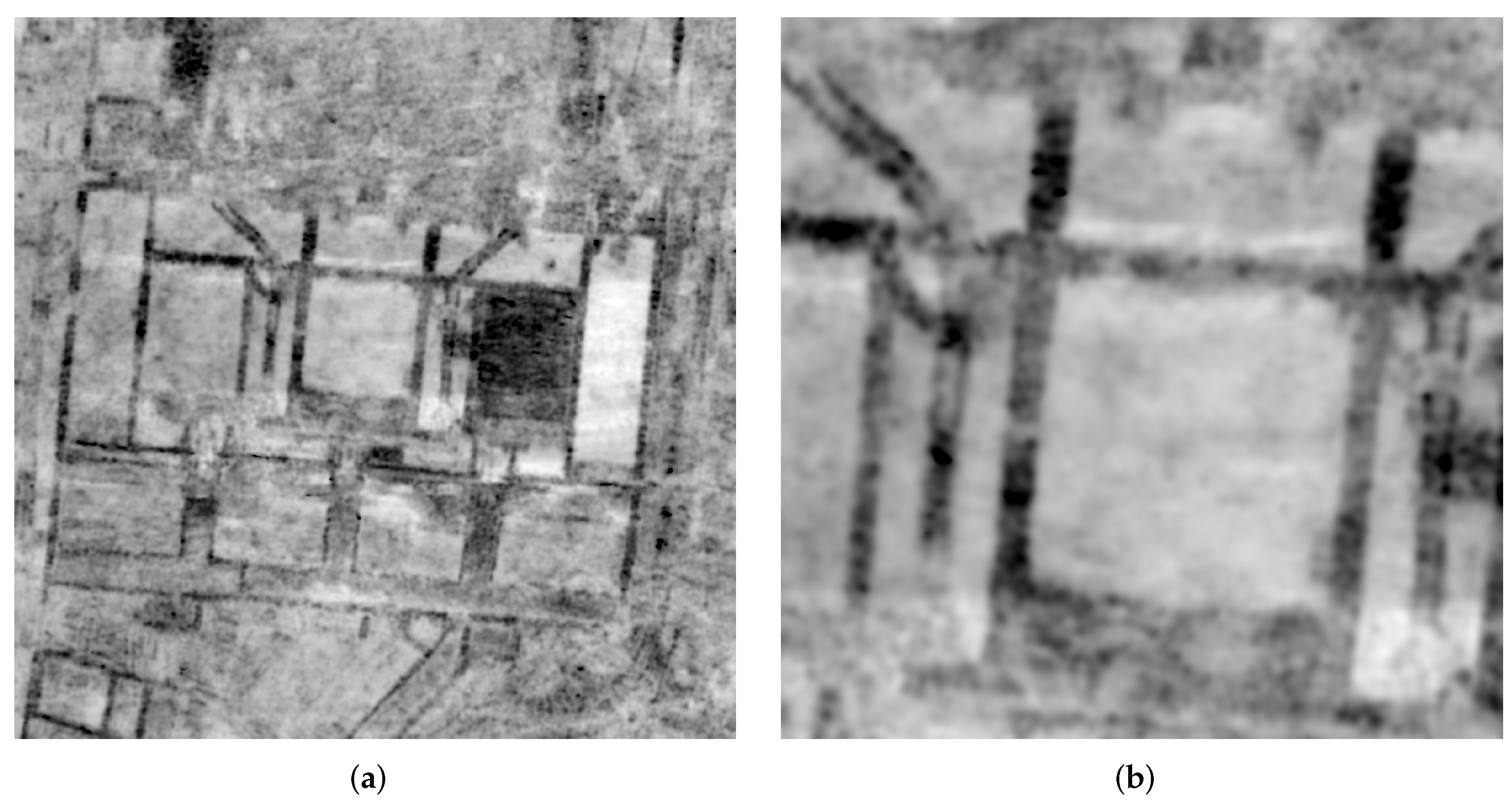
The
bilateral filter, an extension of
Gaussian smoothing preserves major discontinuities, while smoothing the image. This is achieved by weighting the contributions of neighbor values based on their distance in data value space, therefore radar reflectivity, in addition to the weighting in 3D Euclidean space according to Equation (
1) [
42].
Filtered image values at position p are evaluated to the weighted sum of values at positions q in a neighborhood S, where and denote the weights for center voxel and image value distance, respectively, based on Gaussian distributions with standard deviations and . The weighting by proximity in value space largely avoids smearing across structure boundaries, since smoothing is mostly performed using dataset values close to the center value .
Experiments performed with the reference GPR dataset from the forum of Roman Carnuntum showed, that the bilateral filter preserves sharp borders of larger structures, while noise is reduced and small low contrast structures disappear. A median filter of the same kernel size inevitably leads to a higher degree of blurring. Depending on the choice of
many small structures such as sewerage ducts can also be preserved as shown in
Figure 5.
Anisotropic diffusion filters are another type of filters, which can be used to achieve smoothing without sacrificing dataset edge features. The general idea behind anisotropic diffusion filters is to remove noise from images by solving a heat equation (partial differential equation) of the form
with
D denoting the diffusion speed through the medium and
the initial image. With
D set to a constant, solving the above PDE system leads to isotropic behavior such as ordinary smoothing filters; therefore, in [
43]
D was replaced by an edge detector of the form
leading to an inhomogeneous but still isotropic diffusion, which preserves edges by limiting smoothing near them.
Weickart used the structure tensor
to achieve true anisotropic behavior by aligning the diffusion with the local surface structure [
44,
45]. Results differ depending on how this is achieved.
Edge enhancing diffusion (EED) largely inhibits diffusion flow and therefore blurring in surface normal direction, and thereby facilitates edge-preserving smoothing [
46]. Other variants such as
coherence enhancing diffusion steer diffusion along line structure to, e.g., reconnect interrupted line structures.
Application to GPR data shows that EED filters can remove noise from small structures in GPR data. Loss of outline detail through smearing is less prominent than using the median filter as shown in
Figure 6.
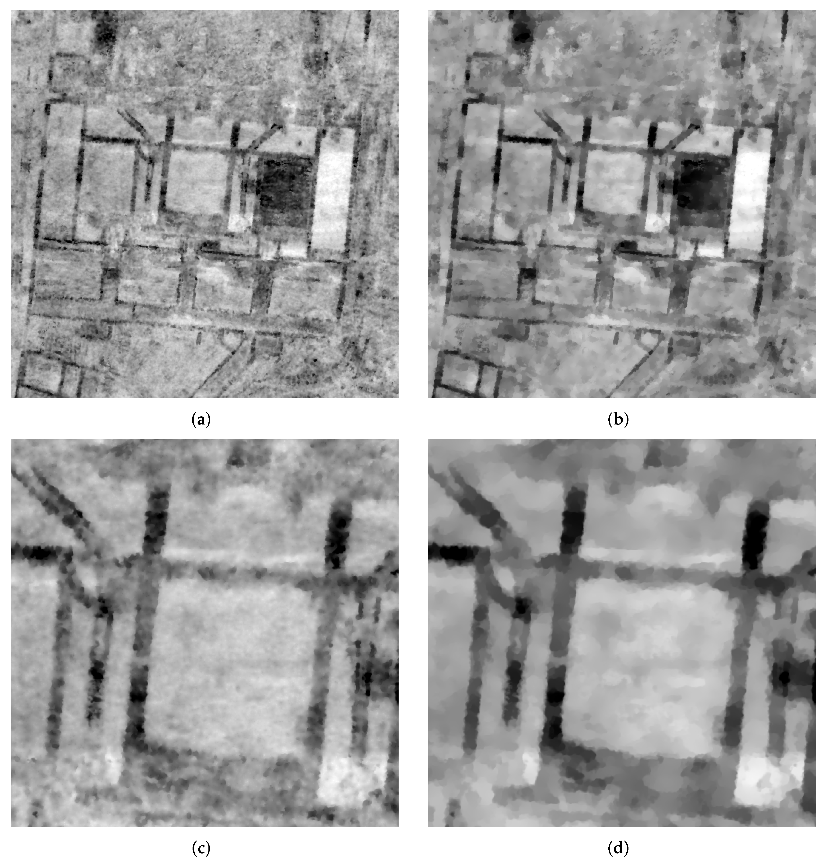
Another state-of-the-art class of methods for edge preserving image denoising are models formulated using the total variation (TV) as first presented in [
47]. Their ROF denoising model uses an energy functional, which consists of a term penalizing differences between the initial image
f and the denoised image
u based on the Euclidean norm (L2), and a second term penalizing high dataset variations. This model leads to an energy minimization problem of the form
The parameter
can be used to trade data fidelity against smoothness of the solution. In [
48] a modified functional model using the L1 norm was proposed.
For both formulations, low values for
lead to a high degree of smoothing. Only the contours of major structures are preserved, while higher
values also preserve small details by penalizing differences to the original dataset.
In our experiments with archaeological GPR datasets their TV-L1 denoising model formulation consistently produced images better suited for 3D visualization than the original ROF model, which is ideally suited for removing Gaussian noise. Small soil structures such as individual stones visible in GPR dataset appear to resemble so-called
salt and pepper noise. This type of noise can better be dealt with by applying the L1 norm, which is known to be robust against outliers. The TV-L1 model also has the advantageous property, that the value of
is proportional to the minimum size of the features to be preserved. Applied to GPR datasets this leads to highly homogeneous and sharp delineation of features supported by the
setting. The dataset values of inner structures converge to a representative mean value. Smaller structures and noise are suppressed as shown in
Figure 7. All in all, the resulting datasets are much better suited for direct volume visualization.
Image filtering is performed using the enormous computing power of modern GPUs. Since all the above-mentioned methods are parallelizable, the achievable speedups are on the order of 100 compared to a CPU implementation, reducing practical computation times for complex iterative algorithms such as TV-L1 denoising from minutes to seconds for practical grid sizes such as the Carnuntum dataset (1601 × 1601 × 50 voxels). Simple algorithms such as the kernel-based bilateral filter can be computed in less than a second. In the presented solution, filtering on the GPU is integrated with the 3D visualization, which allows for interactive tuning of filter parameters.
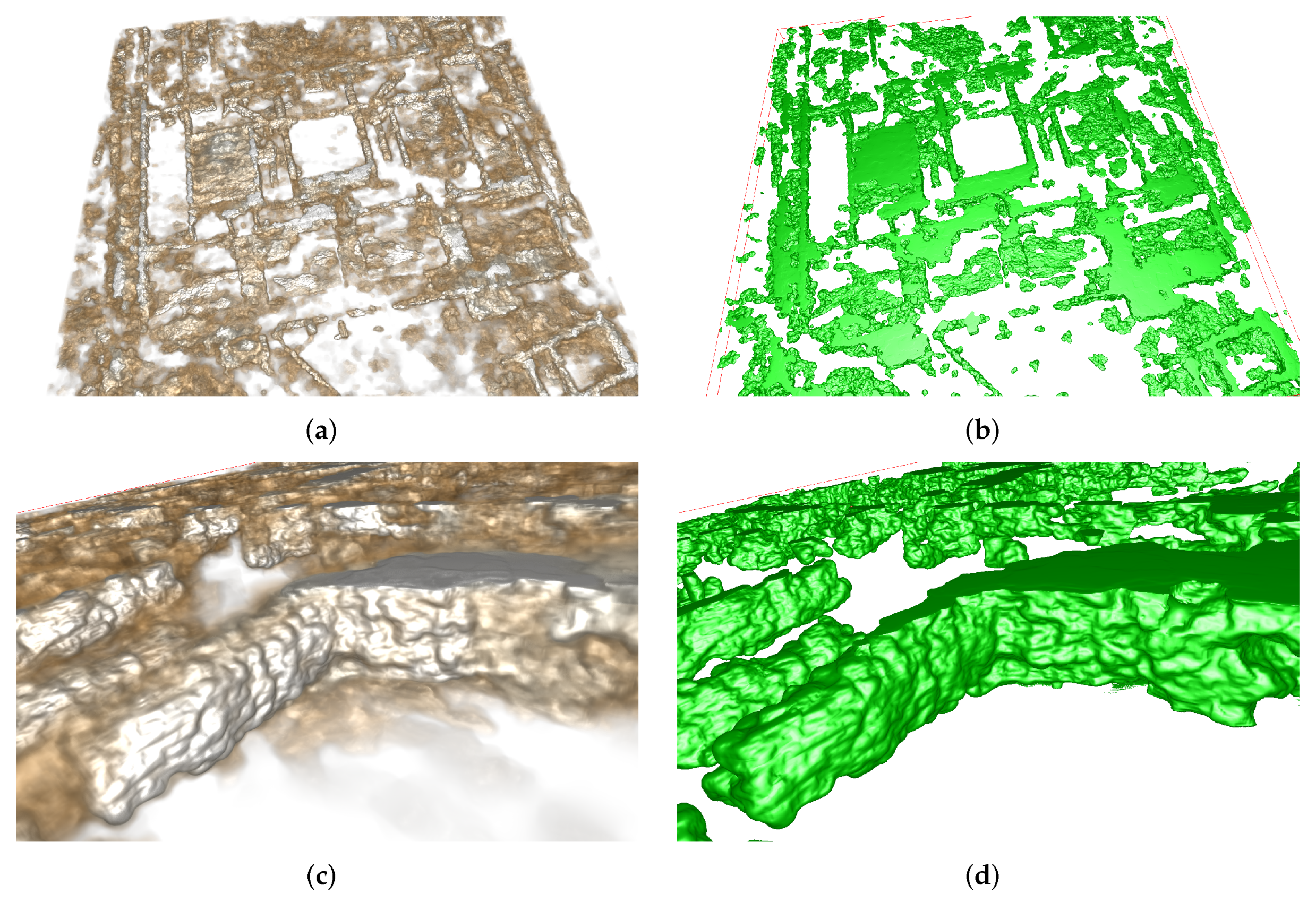
2.3.2. 3D Visualization of Filtered GPR Data Volumes
The filtering algorithms introduced in
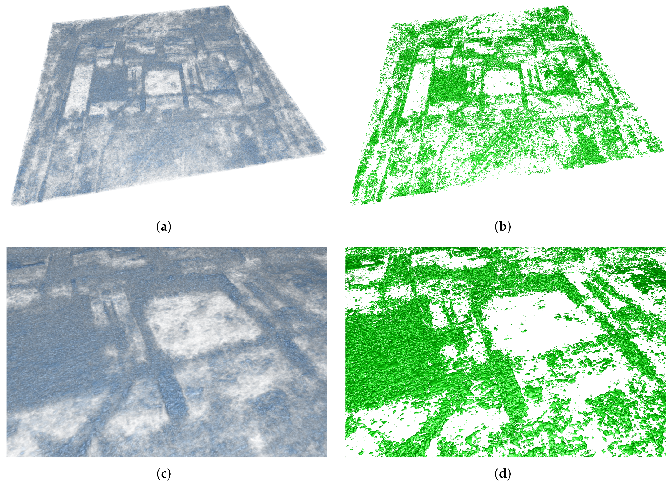
Section 2.3.1 increase dataset homogeneity as required for contiguous volume visualizations of, e.g., the walls of a building. These algorithms remove high frequency noise. Edges of large structures become more clearly defined. This has a significant impact on the 3D visualization output. The 3D shapes of major structures can immediately be seen in both DVR (
Figure 8) and iso-surface rendering (
Figure 9). Building outlines appear at the first glance, which allows further investigations of details such as doors and floors. Occlusion due to the aggregations of small structures still occurs but is by far less disturbing than in the DVR results obtained with unfiltered GPR data in
Figure 4.
With conservative parameter settings the filters just reduce noisy patterns within the archaeological stratification and the geological background. More aggressive parameter settings, such as larger kernel sizes for the median,
, and
for the bilateral filter, a higher number of iterations for the EED filter, respectively, also lead to an increasing degree of structure surface blur, which is usually undesirable. The TV-L1 steps out of the line in preserving sharp transitions at structure boundaries even for small
values, only preserving large structures. By tuning the parameter for a specific structure size, e.g., wall width, the filter virtually removes all smaller structures. Surface details are still preserved. The illustration in
Figure 10 gives the impression that individual stones within the walls become visible. To confirm this, however, an excavation would have to be performed.
We mainly use the TV-L1 filter for visualization in the interpretative process. Experiments beyond the scope of this work have confirmed that it consistently maintains the highest level of detail. Furthermore, it is easy to tune. For other purposes such as preparing GPR datasets for 3D printing, a higher degree of smoothing might be desirable.
2.4. GPR Segmentation
Image filtering greatly aids the quality of 3D GPR data visualization; however, neither the global classification by value of DVR nor the implicit thresholding by iso-surface rendering are able to depict individual features, such as the walls of a single building in a dataset containing many buildings or features characterized by similar dataset values.
In digital image processing nomenclature
segmentation refers to the process of assigning labels to the individual pixels/voxels in an image or dataset sharing certain characteristics such as similar data values, or belonging to the same archaeological entity, e.g., the foundation or the paved floor of a Roman building. Strictly speaking, the binary classification on thresholding by value in iso-surface visualization is already a simple form of segmentation, although with limited capabilities. Thresholding is not powerful enough to separate archaeologically relevant structures in GPR data, since the respective data value ranges are not unique. In medical imaging advanced segmentation techniques using image features and statistics, texture information, and prior knowledge about the target structure can delineate structures such as organs or lesions despite ambiguous data values and noise [
49]. Being able to extract structures of archaeological interest and, ultimately, to divide GPR datasets into archaeologically meaningful non-overlapping labeled features using segmentation techniques would greatly aid the analysis of prospection data. Segmentation approaches applied to GPR datasets could also serve as starting point for the archaeological interpretation process.
Automatic segmentation of archaeological prospection datasets would require the incorporation of existing knowledge and expertise of skilled human interpreters in specific algorithms. The feasibility of such solutions has recently been shown for well-defined problems in medical image analysis, such as the whole heart segmentation. For such problems, state-of-the-art approaches based on deep convolutional neuronal networks (DCNNs) can even outperform human experts [
50]. CNN-based methods learn by example, which requires large training datasets ideally covering all possible data variations due to soil conditions and all conceivable shape variations of the structure to detect or segment. Such training data, archaeological GPR datasets with the target structures manually located and delimited by a human expert, afterwards validated by excavations, do not exist to our knowledge. It is unlikely that they will appear in near future.
To still be able to segment and thereby flexibly extract a variety of structures of archaeological interest from GPR datasets we adopted the interactive segmentation approach in [
48] using an energy minimization functional based on geodesic active contours
, the total variation
of the solution
, and seed regions to be specified by the user
:
This minimization problem can be efficiently solved on GPUs, allowing real-time tuning of the parameters
and
controlling the influence of the gradient of the input image
in
, which generally attracts the solution towards to sharp edges in the input dataset. Parameter
controls the desired similarity to the specified seed region
. Integrated in the visualization framework the seed region image
can be interactively edited by painting constraint regions on top of the input image, thereby efficiently steering the algorithm towards the desired result, whilst avoiding unwanted or missing parts.
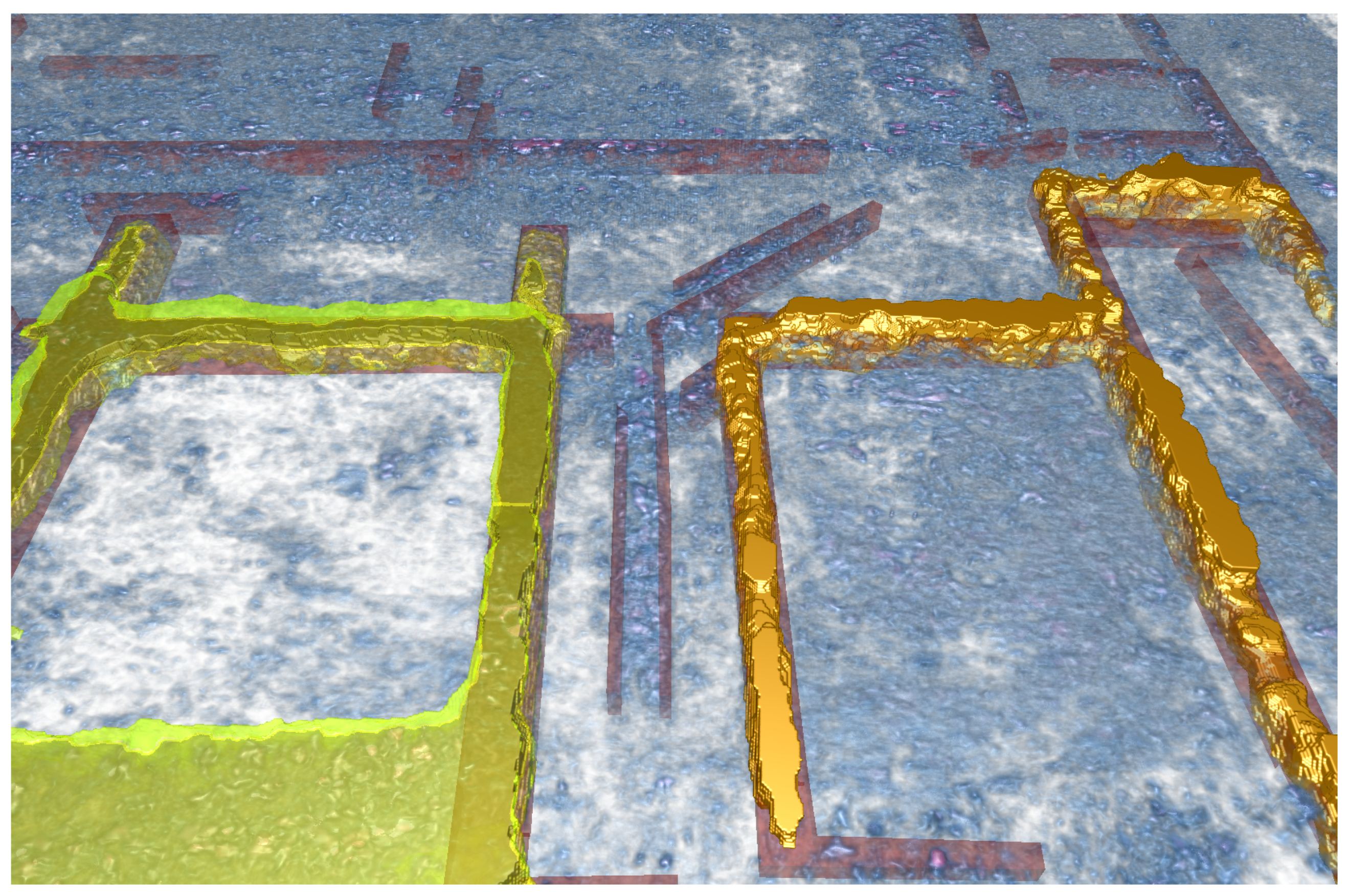
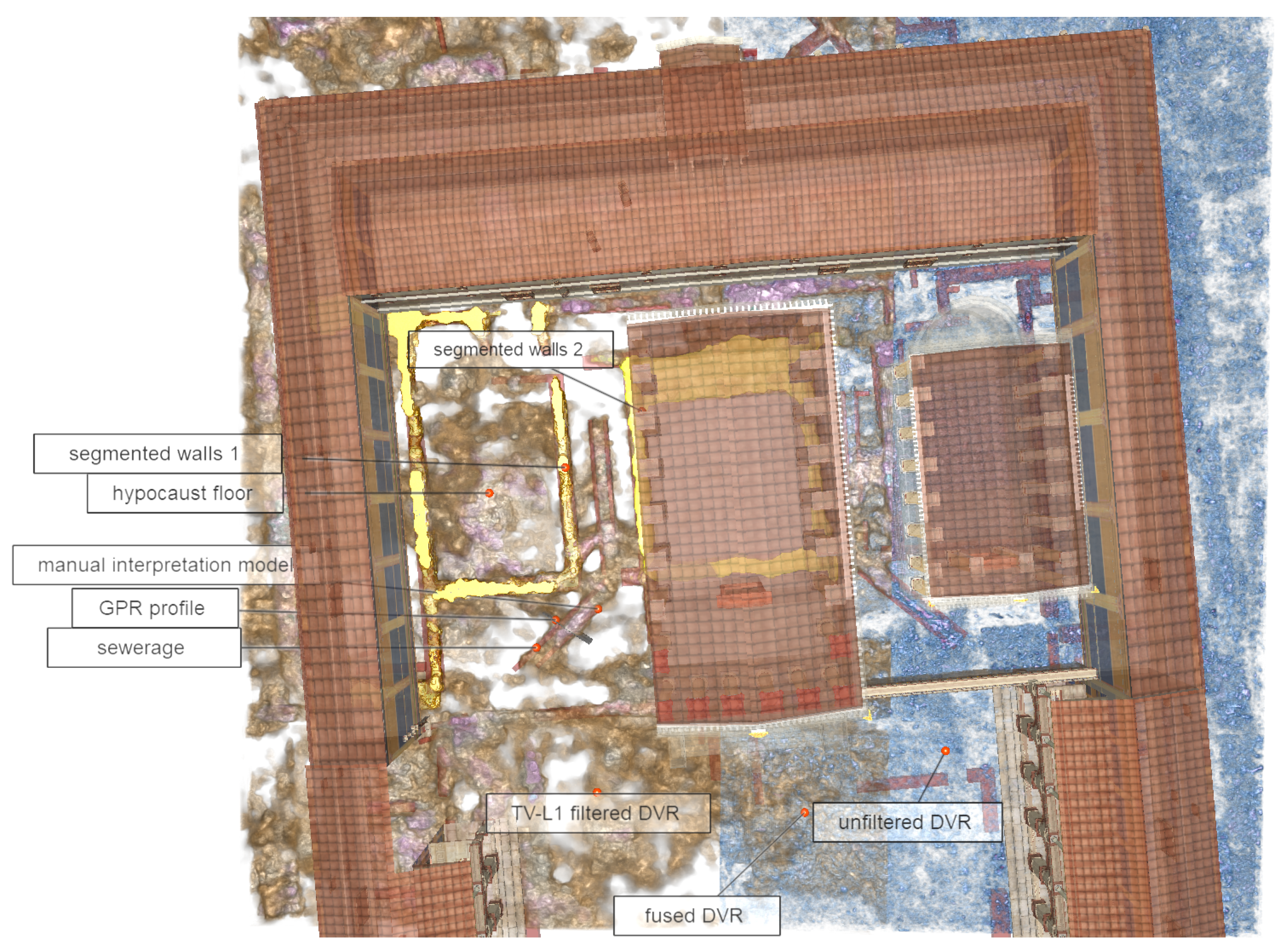
In experiments we tried to segment structures such as barrows, postholes, ditches, and walls including the ones from the forum in Roman Carnuntum. Using this segmentation approach, it was possible to obtain plausible 3D models with little user interaction required. For wall segmentation the outline of the desired building had to be roughly drawn on top of representative GPR slices, which was performed using both, cross-sectional slices shown in the 3D view, and three coupled cross-sectional 2D views of the dataset. For the visualization of the resulting binary segmentation masks, iso-surface rendering was the method of choice.
Figure 11 shows such segmentation results in relation to a manual interpretation model and the underlying dataset.
2.5. Flexible GPR Volume Visualization
The presented visualization system features visualization techniques far beyond DVR and iso-surface visualization. Its high degree of flexibility is achieved using a hybrid rendering algorithm for 3D volume and surface data based on ray-casting, inspired by work presented in [
20], later extended to support conjoint 3D visualization of heterogeneous data in forensic science [
19]. The central idea of the algorithm is to combine the visual contributions of arbitrary datasets passed along view rays through each pixel of the screen in the sense of DVR (see
Figure 2). For each ray, the accumulated output color
and opacity
at sample
i with color
and opacity
are computed using the recursive blending operation in Equation (
7).
In DVR, samples are taken from a single volume dataset. In Equation (
8), we generalize this formulation for samples in
volumes, and include samples at ray intersections with 3D models, where
is the number of volumes or surface samples hit at ray location
i.
While volume dataset samples can be directly obtained from GPU texture memory, meshes, and point sets need to be handled differently. The computation of
and
needs to process their contributions in sorted order with respect to the distance from the viewpoint, which these data types do not support. The HA-buffer presented in [
51] facilitates efficient sorted access to the visual contributions of 3D models using a hash-table, which is populated by rendering the respective models using the OpenGL graphics pipeline. We construct a modified HA-buffer in the first rendering stage, which stores fragment color contributions from visible 3D models. In addition, it handles invisible 3D bounding geometry models for GPR volumes, which can either be quadrilaterals representing the whole dataset range, sub-volumes, or arbitrary 3D shapes. HA-buffer entries from GPR dataset boundary fragments store a signed object ID. The sign distinguishes between entering and leaving the dataset. In the second rendering stage, the HA-buffer is resolved by traversing its depth-sorted stored entries. The objects IDs allow maintaining a set of objects the ray has entered or left, so-called
active objects. Starting with the first HA-buffer entry, visible contributions from surface entries are directly combined with the accumulated color. If a positive object ID is read from the HA-buffer entry, the associated GPR volume is activated until its negative ID is read. The contribution of volumes in the sense of DVR is computed by ray casting and accumulating the samples of all active volumes (Equation (
8)) until the next HA-buffer entry is reached. Multiple contributions at a single sampling location are combined. Implicit iso-surfaces visualization is achieved by detecting iso-surface hits based on two consecutive dataset samples, refining the hitpoint, and inserting the visual contribution as an additional sample.
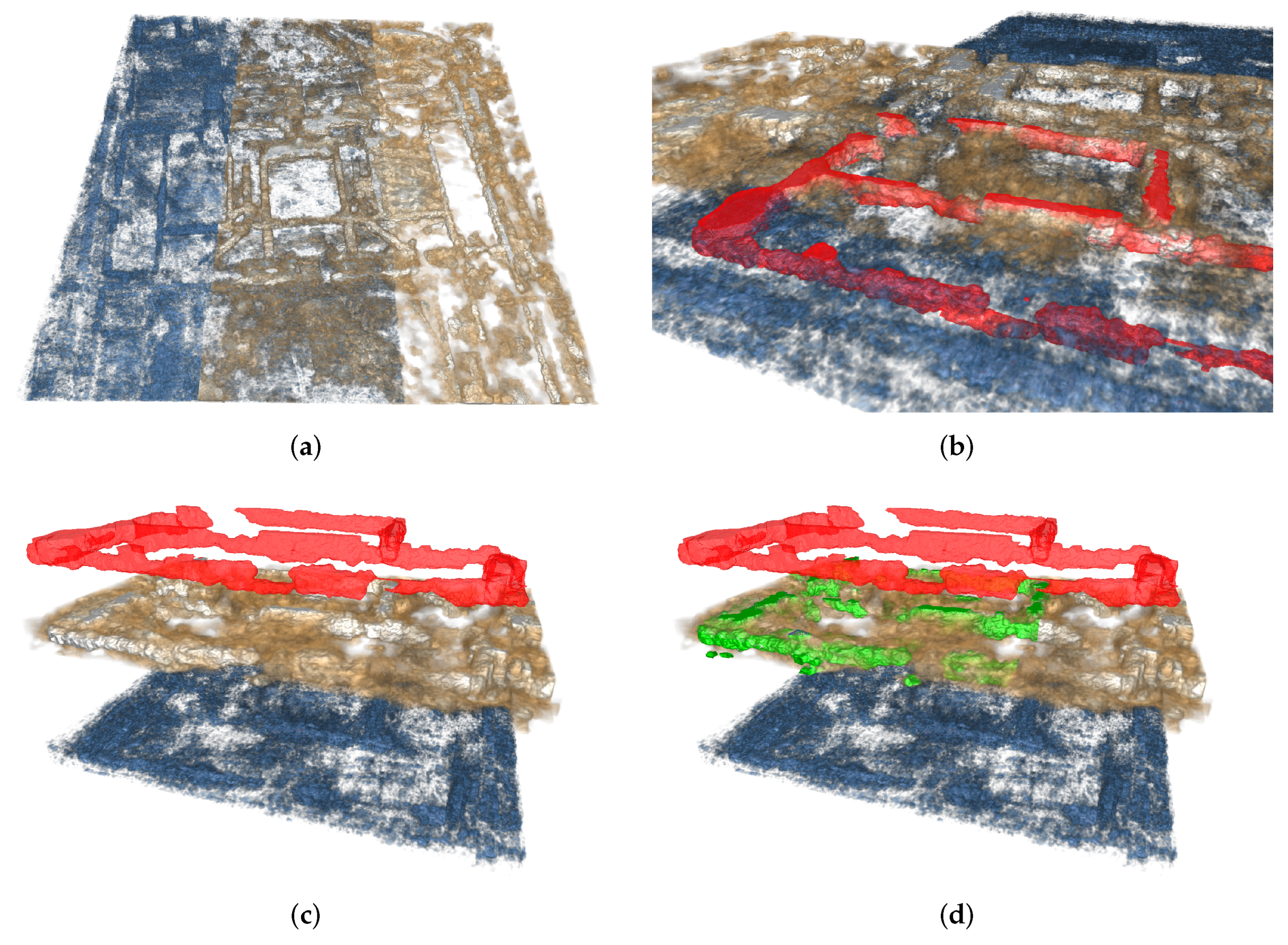
This hybrid rendering for heterogeneous data offers a multitude of possibilities for visualization. Support for multiple volume datasets allows the fused visualization of unfiltered and filtered dataset versions, as well as segmentation datasets. It is possible to independently choose between DVR and/or iso-surface rendering, and their respective visualization parameters. Furthermore, datasets from multiple different measurements can either be superimposed, or visualized next to each other. In our fused visualization approach, the orientations and resolutions of the datasets do not have to be identical. This is particularly useful, if a site is measured at different points in time, or using diverse measurement equipment.
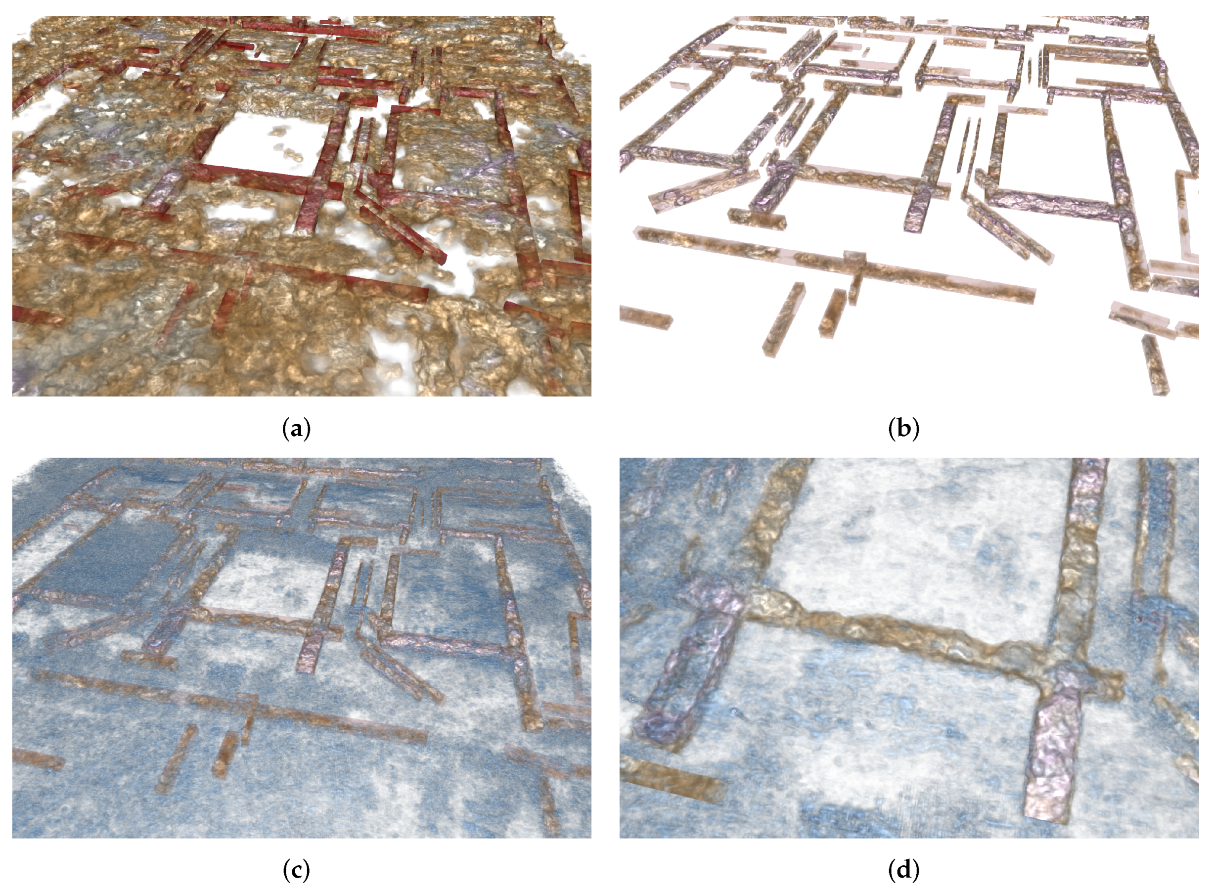
Figure 12 shows examples on how to use this functionality in archaeologically beneficial ways: The superimposition of an unfiltered dataset with a TV-L1 filtered version shows the major features emphasized by the filter. Thanks to the fused visualization approach the details suppressed by the filter can be re-added as visual contributions from the unfiltered dataset. The integration of a segmentation volume displayed as semi-transparent iso-surface allows the detailed analysis of the enclosed volume while being aware of the depicted structure’s shape and extent, in this case, the remains of the wall. Spatially distributed visualization avoids mutual occlusion. Iso-surfaces rendering integrated with DVR may generally be used to further emphasize specific features, such as regions of exceptionally high radar reflectivity or segmentation results. In the example the choice of a high iso-value depicts most of the foundation.
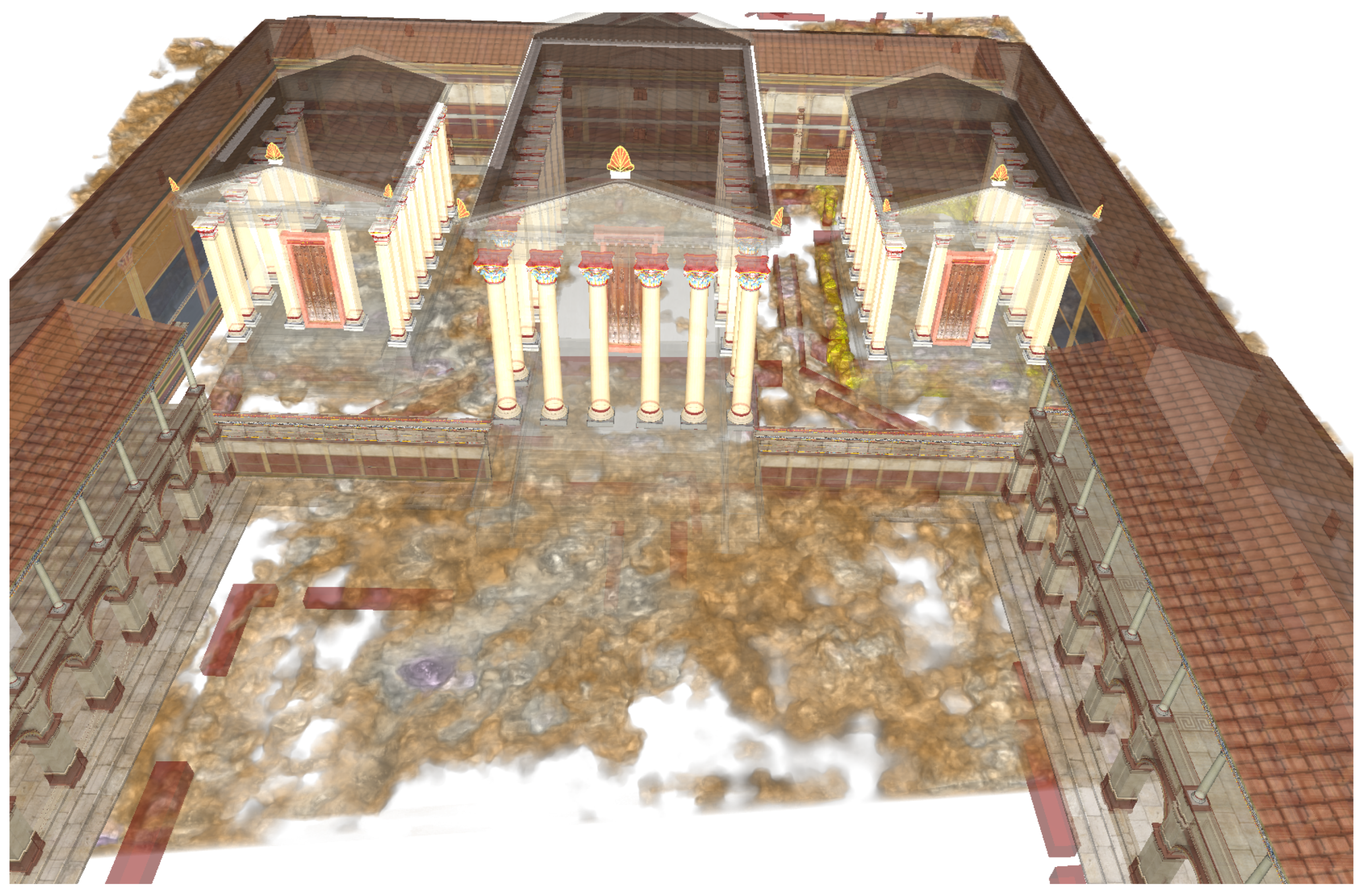
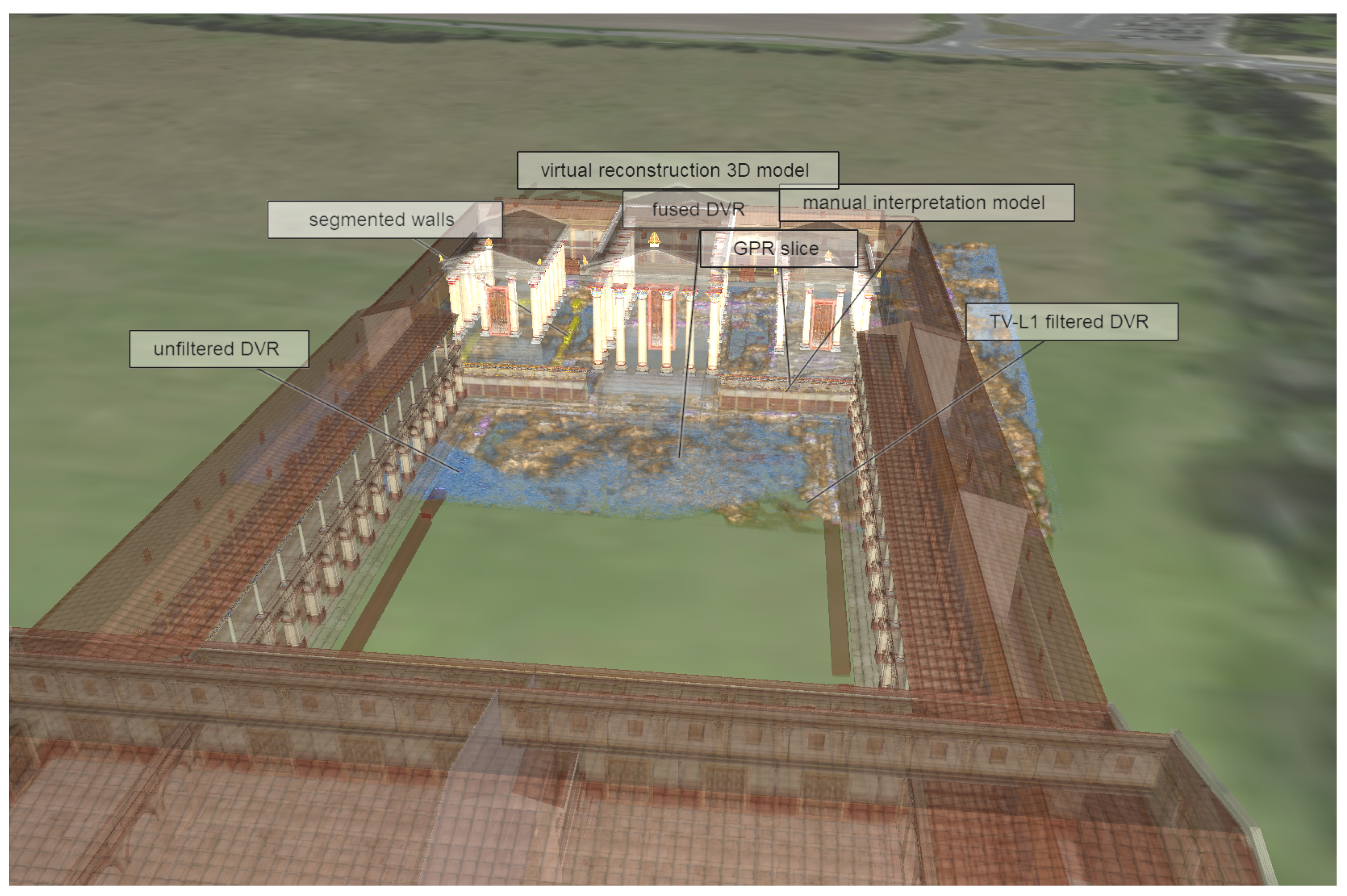
Support for arbitrary 3D data is a key feature of the proposed approach. It enables comprehensive visualizations of measured data and 3D interpretation models converted from interpretations manually elaborated in GIS tools by drawing polygons. The 2D polygons are converted into 3D models by extrusion. The simultaneous visibility of recorded prospection data, computer-aided analysis results, and human reasoning results in unprecedented possibilities for comprehensive prospection data analysis. It has the potential to support the discussion of interpretation results. Such visualizations are a powerful tool for the comparative dissemination of complex interpretation results to non-experts, which may increase their understanding by establishing the link between abstract prospection data and more tangible virtual models.
Figure 13 shows a virtual reconstruction of the Roman forum of Carnuntum together with filtered GPR data and a 3D interpretation model.
2.6. Local Visualization Control
We have shown how to visually combine multiple heterogeneous datasets by accumulating their individual contributions in a fused visualization approach. Still, the possibilities of the proposed method are far from being exhausted. The core rendering algorithm keeping track of the objects encountered along the view rays opens countless new possibilities for even more flexible visualization techniques. Based on the archaeological need to visually depict structures in GPR data, we exploited the feasibility of application domain control for DVR using 3D models, thereby extending work in [
19]. The simplest form of geometry-based visualization control is to restrict DVR to volume regions inside or outside a 3D model. It is also possible to use different DVR parameters leading to a different DVR appearance in the intersection region. Another option is to select the displayed dataset version (filtered or unfiltered) depending on the location relative to the controlling 3D model.
Our implementation supports restricting the visible portion of the dataset based on constructive solid geometry (CSG) operations. CSG techniques are routinely used in the CAD domain to model complex mechanical parts by applying a series of intersection, union, and difference operations with simple geometric primitives to an initial geometric model, e.g., a difference operation using a cylinder to model the drilling of a borehole into an existing 3D model.
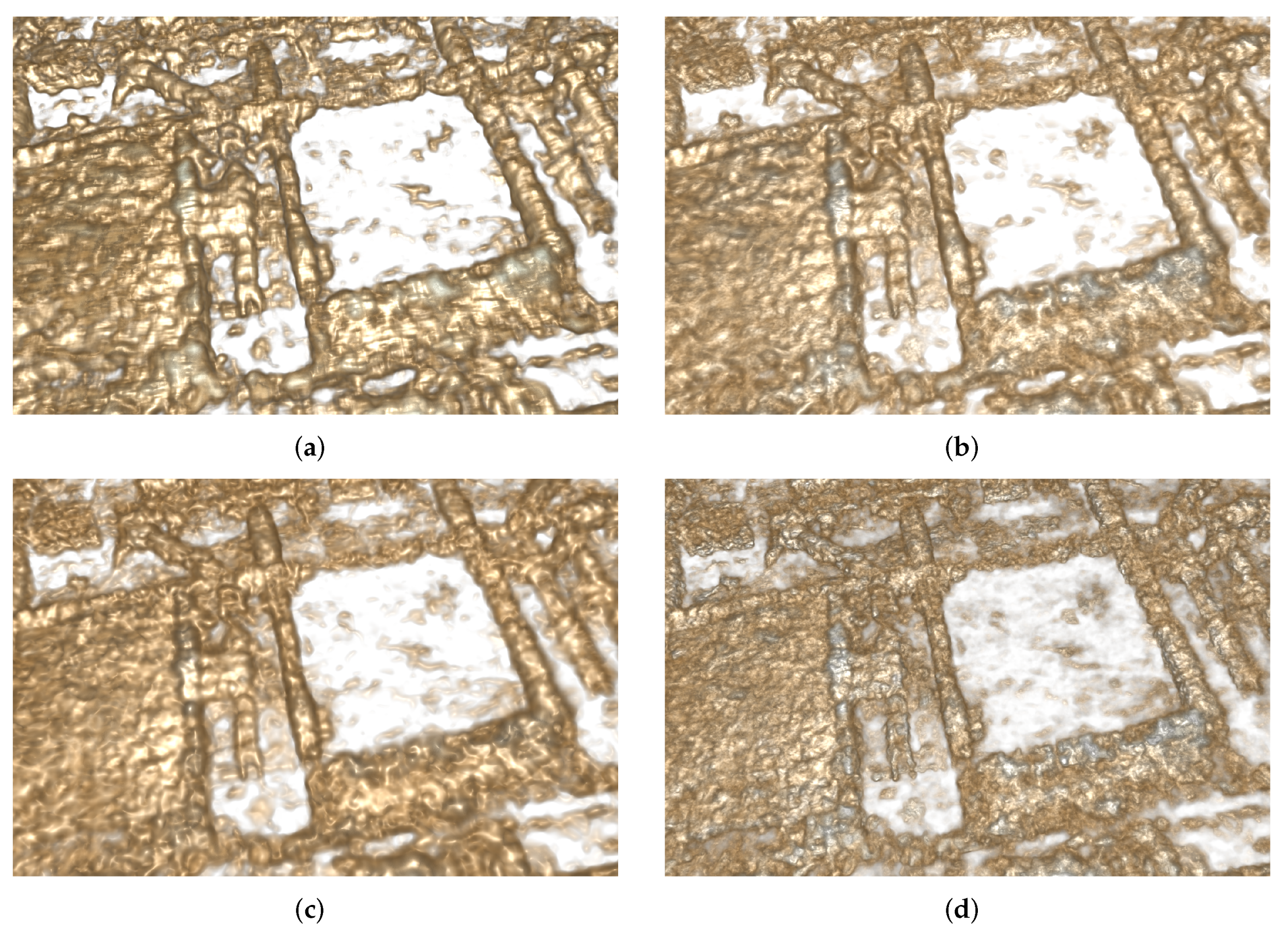
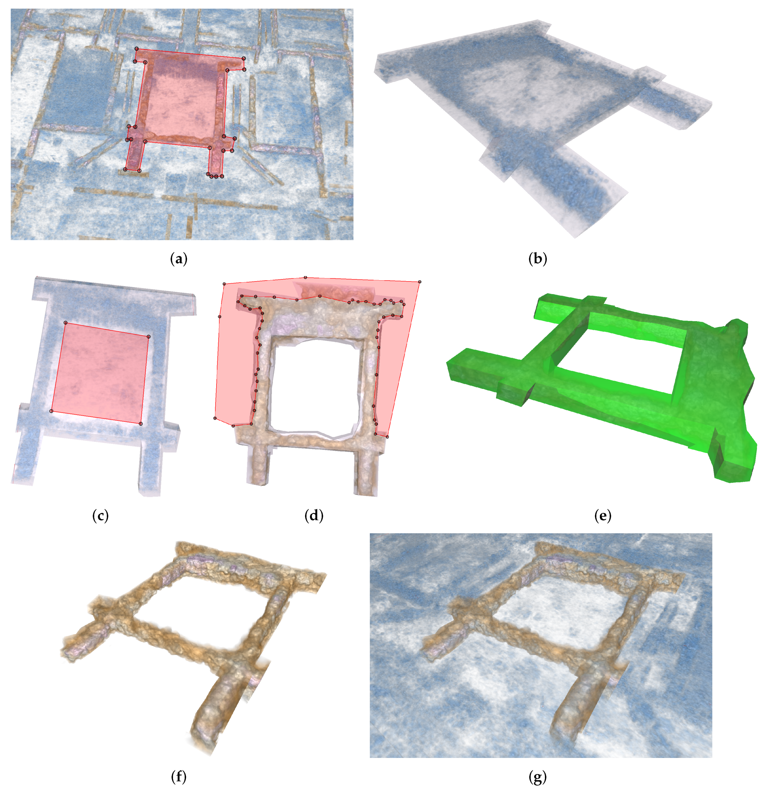
Figure 14 shows a local visualization control example using a simple 3D interpretation model, depicting walls and sewers. Instead of displaying the 3D model and the GPR dataset together (
Figure 14a), the invisible 3D interpretation model geometry is used to restrict GPR DVR to its extents. This way, surface details of the dataset features in the selected portion of the filtered GPR dataset can clearly be seen, while occlusion by visual contributions from outside the interpretation boundaries does not occur at all (
Figure 14b). Another option is to show outside dataset regions using a different transfer function. In the example both, i.e., an unfiltered version of the dataset and a different transfer function were used. Walls with well-defined contours stand out in the resulting images, while the surrounding dataset remains visible (
Figure 14c,d).


