Multidecadal Land Water and Groundwater Drought Evaluation in Peninsular India

Abstract

To efficiently mitigate the multitude of direct and indirect impacts, basin-scale drought characterization is imperative, particularly for India, where water scarcity is continually increasing. We jointly used the GRACE gravity data, PCR-GLOBWB model outputs, and in situ data to quantify the deficits based on land water storage (LWS) and groundwater storage (GWS) in Peninsular India for 35 years from January 1980 to December 2014. The results showed that the study basins experienced high interannual variations despite the minimal linear LWS trends (0.26–0.56 mm yr⁻¹). GWS showed a slow but persistent response (longest deficit spanning ~6 years) to the seasonal variations in the hydrological fluxes and remained the major contributor to LWS. We demonstrated (1) the potential of the PCR-GLOBWB model to analyze LWS and its segregated components beyond GRACE data records, (2) the LWS-based index as a better drought indicator than traditional drought indices, and (3) GRACE-LWS as a proxy indicator of real-time groundwater monitoring without relying upon the intermittent in situ observations. This study underscores the need to revise the water allocation strategies and irrigation systems to maintain the sustainability of groundwater systems and may serve as a holistic framework for remotely monitoring the water beneath our feet, especially in the data-limited regions globally.

1. Introduction

Droughts, primarily a form of the water deficit conditions, cause significant impacts on various sectors, including food security, public health, ecosystems’ stability, freshwater availability, and socio-economic development in a region [1,2]. The impacts of droughts are evident in almost every region and climate, spanning from the tropical parts of Asia to the historic cities of Europe, with varying meaning and significance [3,4,5]. The joint influence of the population growth-induced water demands and climate change, which is expected to increase the areal extent, intensity, duration, and frequency of droughts globally in the near future [6,7], has drawn the attention of researchers in hydrology and associated disciplines [8]. The cascade of drought, i.e., the propagation of water deficit, from precipitation (meteorological) to soil moisture (agricultural) and streamflow (hydrological), ultimately affects the groundwater storage, leading to a distinctive class of drought called groundwater drought [8,9,10]. However, compared to the (near)-surface water storage components (surface water and soil moisture), an accurate assessment of the groundwater (GW) dynamics and the embedded water deficit conditions, which are not commonly visible, is still challenging, especially at the regional scales and for multidecadal time scales.

Groundwater accounts for about 98% of the global freshwater resources, excluding glaciers and ice-caps, making it a vital source for meeting environmental and human-induced water demands [11]. However, there has been unprecedented stress on the groundwater resources due to overexploitation, which has resulted in, for example, the depletion of ~330 km³ of GW in the High Plains Aquifer in the U.S. (from 1950 to 2007) [12] and ~140 km³ over the California Central Valley (from the 1860s to 2003) [13]. This stress is not limited only to the dry regions where a limited amount of surface water is available but also extends to the areas with abundant rainfall where multiple attributing factors exist, such as the spatiotemporal heterogeneity in precipitation, poor management and pollution of surface water resources, and population growth, causing over-reliance on the GW [9]. Further, the existing low resiliency makes quantification of the multidecadal groundwater resources dynamics of prime importance for the (semi)-arid regions, such as Peninsular India, where the GW abstractions primarily govern the regional food security and socio-economic stability [14,15].

India is the world’s largest user of groundwater at an annual rate of 230 km³, which is over a quarter of the global total, 90% (much higher than the global average of 40%) of which is used for ~60% (global value: 38%) of the total irrigated land in the country. The remaining 10% is used in meeting ~80–85% of the water demands of ~90 million rural households [16,17,18]. This high dependence on GW resources in India has resulted in half of the country’s area already suffering from water stress conditions with a meager per capita share of water storage [19]. Assessment of the in-situ groundwater data collected by India’s agency Central Ground Water Board has revealed that 42% of GW wells experienced a decrease in water level, with 7% showing a decline of as high as 2–4 m between 2001 and 2011 [20]. Furthermore, the ratio of groundwater consumption to recharge increased to 62% in 2011 from 58% in 2004 in the country [19,21].

Several inherent hindrances in in situ data comprehension, mainly caused by the inadequacy of the monitoring network, recorded data gaps, and discrete spatial representation, among others, limit the holistic characterization of the groundwater storage solely based on actual field observations [22]. Notwithstanding the hindrances, satellite observation (especially, Gravity Recovery and Climate Experiment, i.e., GRACE) jointly assimilated with auxiliary data from the global hydrological models (e.g., PCR-GLOBWB) has proven quite promising to quantify the hydrological cycle components on the required spatial and temporal scales globally in the past decade [23,24,25,26,27,28,29,30,31]. However, all of these studies focus on the brief observational records coinciding with the GRACE, i.e., from April 2002 onwards, and the water storage dynamics with an explicit focus on groundwater, to the best of our knowledge, remains largely unexplored beyond the GRACE records. Therefore, in this study, we characterize the multidecadal (1980–2014) water storage deficits in both land water storage (LWS) and groundwater storage (GWS) and subsequently analyze the droughts in terms of magnitude, duration, severity, and recovery time in Peninsular India where the water scarcity has recently been increasing (Figure 1, Supplementary Section S1).

The major contribution of the current study is as follows. First, the multidecadal study period (35 years) provides insights into the long-term slow systemic changes in the hydrological system of a cumulative catchment area of 709,151 km² (~22% of the geographical area of India), providing a blueprint for future climate change studies. Secondly, we demonstrate the applicability, with embedded model uncertainties, of the PCR-GLOBWB model to simulate the integrated and segregated water storage components beyond the GRACE satellite and subsequently show the superiority of the LWS-based deficit index (Supplementary Section S2) over traditional indices. Thirdly, to address the challenge for a real-time monitoring framework imposed by the irregular groundwater measurements, we propose the water storage deficit index (WSDI) as a potential proxy near-real-time indicator of the groundwater drought index (GWDI) and that can subsequently be utilized for early GW drought warning systems. Given the robust but straightforward approach, the current basin-scale decadal drought characterization framework can be employed globally in various data-scarce or data-limited river basins.

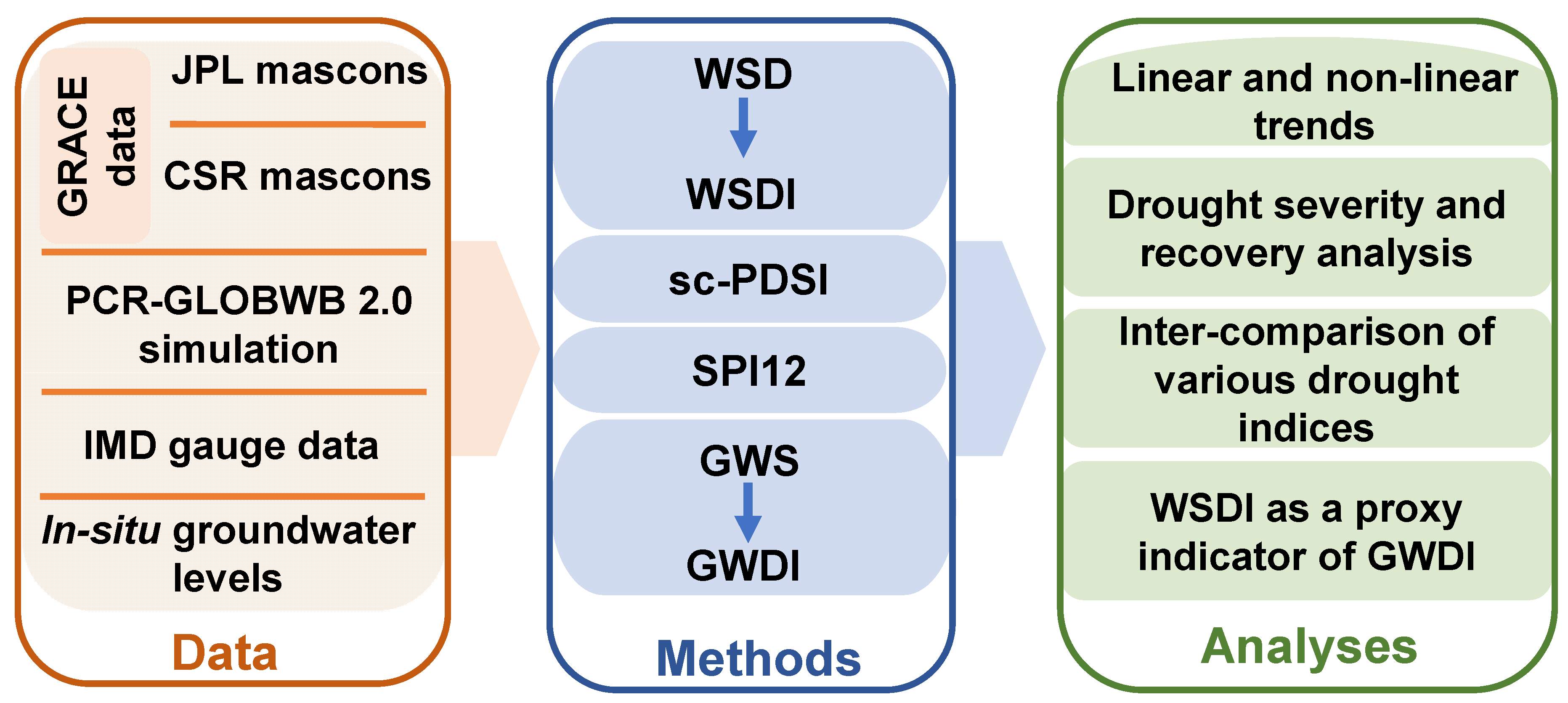
2. Materials and Methods

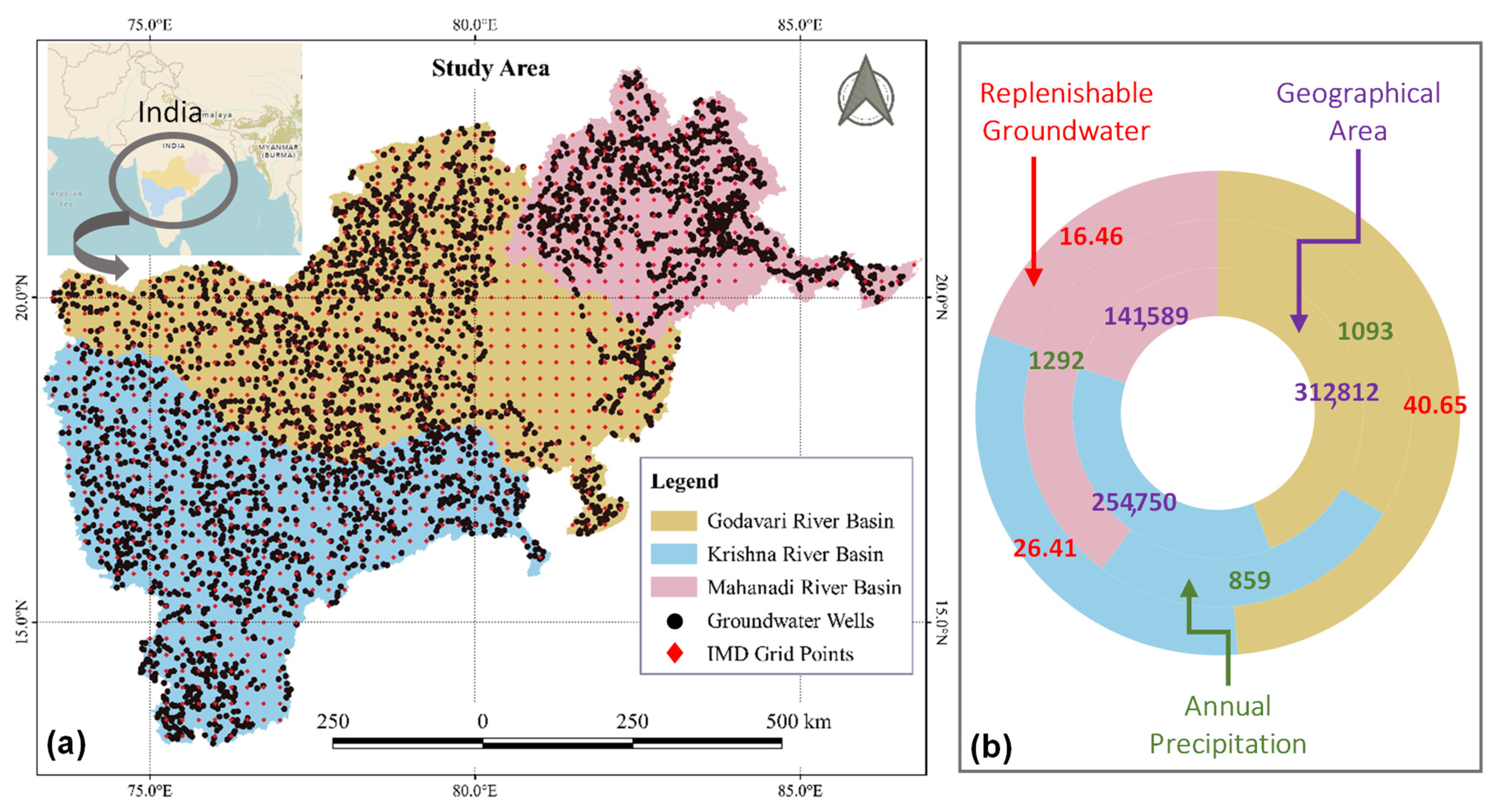
2.1. Study Area

Three river basins, namely, the Godavari, Krishna, and Mahanadi river basins (abbreviated as GRB, KRB, and MRB, respectively), were selected for the study (Figure 1,

Table 1. Salient features of the three study basins. Three river basins selected in the study and their geographical area, basin-averaged precipitation for January 1980 to December 2014 [34], population statistics [33], water scarcity situation [34], and the maximum groundwater level (GWL) depth as per the observational wells used in this study.

River Basin	Geographical Area (km2)	Mean Annual Rainfall (mm)	Variability (Min.–Max.) in Rainfall (mm)	Estimated Population (Million)		Estimated Per Capita Water Availability (m3)		Current Category *	No. of Wells †	GWL Depth (m)
				2025	2050	2025	2050
Godavari (GRB)	312,812	1093	400–2500	89.18	104.92	1320.25	1122.19	Water stressed	430	33.6
Krishna(KRB)	254,750	859	100–4000	100.41	118.13	886.76	753.75	Water scarce	515	47.8
Mahanadi (MRB)	141,589	1292	1080–1653	43.93	51.68	1661.73	1412.54	Water stressed	135	34.4

* The estimated per capita water availability is below 1700 m³ in the GRB and MRB, which are under water-stressed conditions, and below 1000 m³ in the KRB, which is under water-scarcity conditions [34]. † represents the total number of wells after filtering for each basin (Supplementary Section S7d).

). Compared to the national mean annual rainfall (1200 mm), these basins receive a limited amount (for the GRB and KRB) or a fair amount (for the MRB) of rainfall, of which 80 to 90% occurs during the monsoon season (June–September). The dependency of water supply on the groundwater in all three basins is more than 70%, which is likely to be increased in the future due to the continuously rising groundwater consumption [32,33]. Moreover, inadequate public water supply systems and advanced pumping and drilling technologies may further intensify the unsustainable groundwater extraction, often through unregistered wells, in the area. A summary of various salient features of the study basins is shown in Table 1 and a schematic of the methodology and various research components of this study is shown in Figure 2.

2.2. Water Storage Components and Climate Data

The high-resolution (0.25° × 0.25°) daily gridded precipitation data, which have been developed by using a network of 6955 rain gauge stations pan-India, were accessed from the India Meteorological Department for the study duration (https://www.imdpune.gov.in/, accessed on 22 November 2021; [35]). These precipitation data, along with the standard dataset for other hydrometeorological variables, were further used for the forcing PCR-GLOBWB 2.0 model. Time series of various water storage components (WSCs), i.e., soil moisture, groundwater, and routed surface runoff, were simulated using the model from January 1980 to December 2014. All these components were then summed up to obtain the modeled LWS (${\mathrm{LWS}}_{\mathrm{m}}$). For convenience, all the model outputs are named as modeled WSCs (e.g., modeled soil moisture storage; ${\mathrm{SMS}}_{\mathrm{m}}$; similarly, ${\mathrm{GWS}}_{\mathrm{m}}$ and ${\mathrm{LWS}}_{\mathrm{m}}$).

Further, an arithmetic mean of the two GRACE mascon solutions represented as basin-averaged equivalent water depth (mm) was used to compare the model performance in simulating LWS. GRACE-derived LWS represents the integrated sum of canopy water, surface water, soil moisture, and groundwater and has been used in several studies for varying purposes of water budget and water storage dynamics [4,23,28,36]. Overall, an inter-comparison of GRACE LWS shows strong agreement between all products with the variance among different GRACE products ranging within error bounds of the GRACE data with no significant biases, which is consistent with previous studies [37]. As there is minimal signal loss attributed to the regularization and post-fit residual analysis, no signal restoration procedures are required for GRACE Mascon (mass concentration) solutions [28,36].

For more details about the PCR-GLOBWB model attributes and settings and GRACE data, please see Supplementary Sections S3 and S4, respectively.

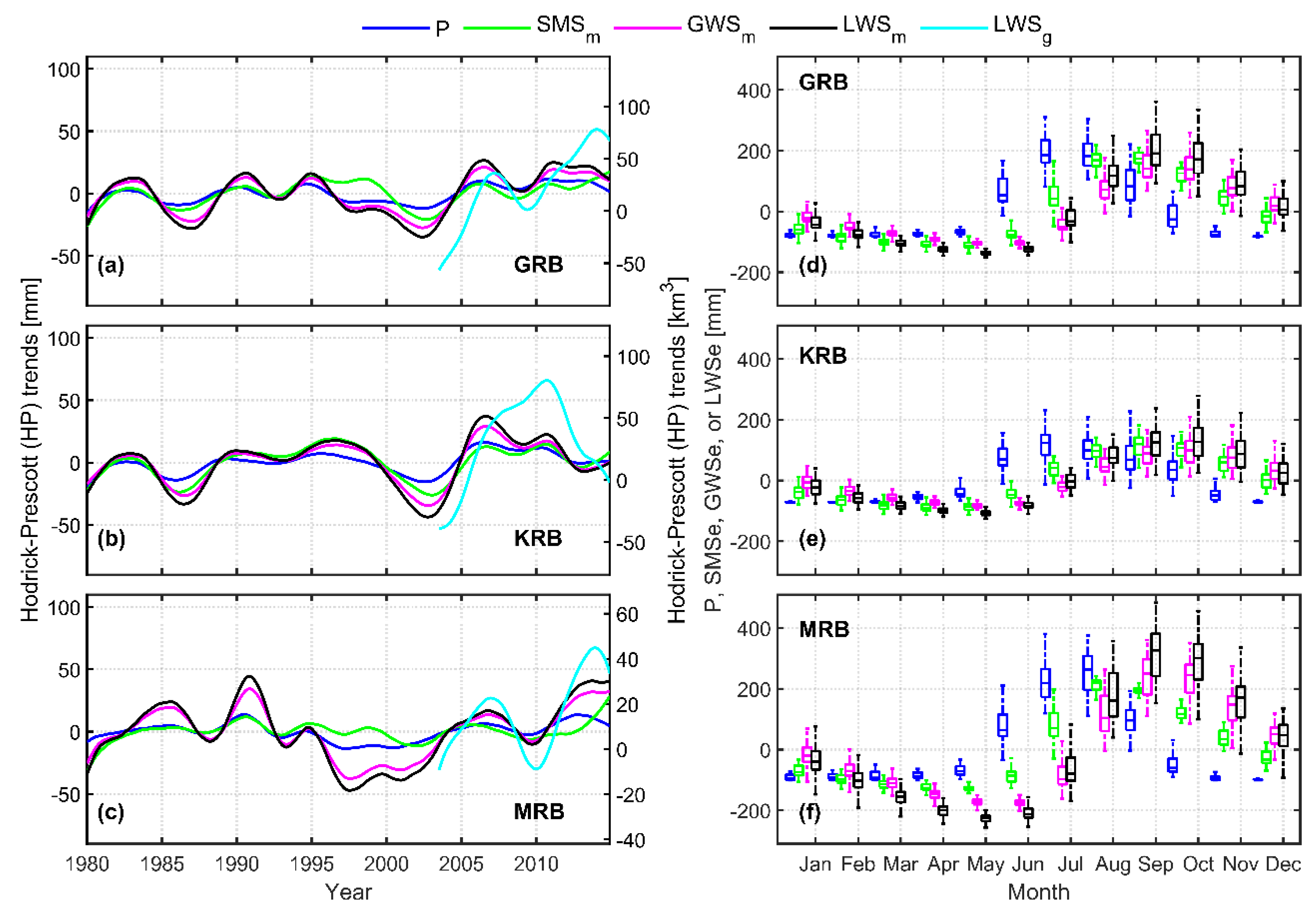
2.3. Linear and Non-Linear Trend Analysis

Although the linear trend analysis gives the long-term change in the basin, the existing nonlinearity in the data has motivated us to use the nonlinear nonparametric trend analysis, namely the Hodrick–Prescott (HP) filter. For a doubly infinite series, the cyclic component was estimated in the given data time series ${\mathrm{y}}_{\mathrm{t}}$ by the high-pass filter [38]:

$$\widetilde{{\mathrm{c}}_{\mathrm{t}}}=\tilde{\mathrm{H}}\left(\mathrm{L}\right){\mathrm{y}}_{\mathrm{t}}$$

(1)

where $\tilde{\mathrm{H}}\left(\mathrm{L}\right)$ is the weight function with $\mathrm{L}$ as the loss parameter (Supplementary Section S5).

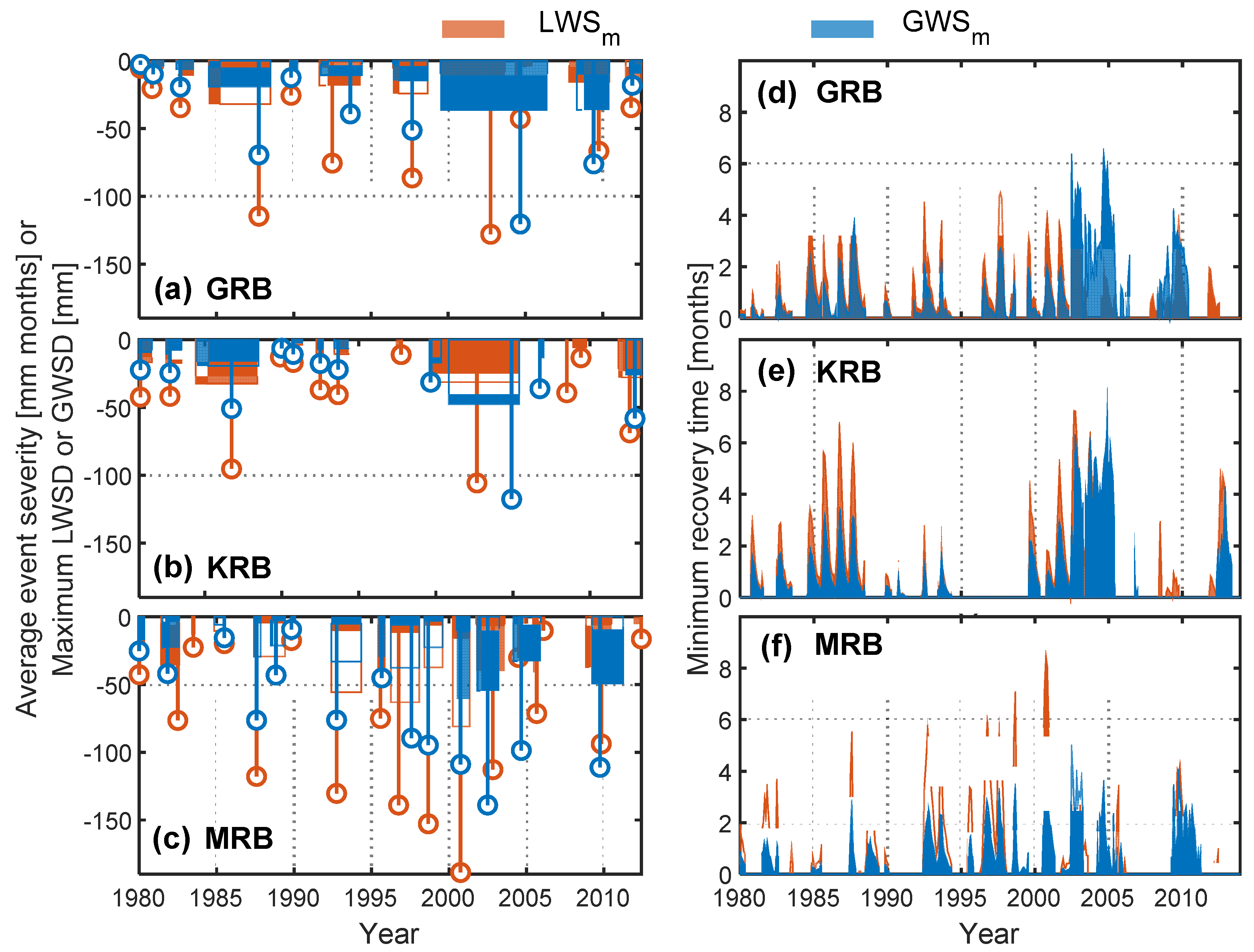
2.4. Drought Severity and Recovery Time

We calculated the monthly events of water storage deficits in both ${\mathrm{LWS}}_{\mathrm{m}}$ and ${\mathrm{GWS}}_{\mathrm{m}}$ by removing their respective climatology and further calculated and inter-compared the event severity and recovery times. We extended the approach by [39] for calculating the deviations (surplus or deficit) from the average conditions, as shown below (example of ${\mathrm{GWS}}_{\mathrm{m}}$):

$${\mathrm{GWSD}}_{\mathrm{i}}={\mathrm{GWSA}}_{\mathrm{i}}-{\mathrm{GWSA}}_{\mathrm{i}}^{\mathrm{c}}$$

(2)

where ${\mathrm{GWSD}}_{\mathrm{i}}$ is the GWS deficit, ${\mathrm{GWSA}}_{\mathrm{i}}$ is the GWS anomaly based on ${\mathrm{GWS}}_{\mathrm{m}}$, and ${\mathrm{GWSA}}_{\mathrm{i}}^{\mathrm{c}}$ is the climatology of GWSA for the ith month. The monthly climatology was calculated as the average monthly GWSA over the study period. Further, the event severity (${\mathrm{S}}_{\mathrm{t}}$) corresponding to each water deficit event (which primarily represents the cumulative ${\mathrm{GWS}}_{\mathrm{m}}$ deficit from the onset of the deficit) was calculated as:

$${\mathrm{S}}_{\mathrm{t}}={\overline{\mathrm{M}}}_{\mathrm{t}}{\ast \mathrm{D}}_{\mathrm{t}}$$

(3)

where ${\mathrm{S}}_{\mathrm{t}}$ is the event severity (mm months), and ${\overline{\mathrm{M}}}_{\mathrm{t}}$ (mm) and ${\mathrm{D}}_{\mathrm{t}}$ (months) are the average water deficit in ${\mathrm{GWS}}_{\mathrm{m}}$ and duration since the onset of the deficit period, respectively. The same procedure (Equations (2)–(4)) was applied for ${\mathrm{LWS}}_{\mathrm{m}}$-based calculations. For understanding the drought recovery, we further calculated the time to recover from below-normal storage conditions (Supplementary Section S6, Figure S1).

2.5. Standardized Indices

We utilized four types of standardized indices to assess the temporal extent and variability of the basin-scale droughts in multiple water storage or hydrometeorological components and assessed the model’s potential to simulate individual WSCs. These indices included the self-calibrating Palmer Drought Severity Index (sc-PDSI) [40], 12 month Standardized Precipitation Index (SPI12) [41], normalized water storage deficit index [4] (WSDI; ${\mathrm{WSDI}}_{\mathrm{m}}$ based on ${\mathrm{LWS}}_{\mathrm{m}}$ and ${\mathrm{WSDI}}_{\mathrm{g}}$ based on ${\mathrm{LWS}}_{\mathrm{g}}$), and normalized groundwater drought index [9] (GWDI; ${\mathrm{GWDI}}_{\mathrm{m}}$, ${\mathrm{GWDI}}_{\mathrm{g}}$, ${\mathrm{GWDI}}_{\mathrm{o}}$; Supplementary Section S7e). Please note that the subscripts m, g, and o represent the indices derived from the modeled, GRACE-derived, and observed in situ data, respectively. For all WSDIs and GWDIs, the zero-mean normalization procedure was followed, as shown below (example of GWDI):

$${\mathrm{GWDI}}_{\mathrm{j},\mathrm{k}}=\frac{{\mathrm{GWSD}}_{\mathrm{j},\mathrm{k}}-\mathsf{\mu }}{\mathsf{\sigma }}$$

(4)

where ${\mathrm{GWDI}}_{\mathrm{j},\mathrm{k}}$ is the normalized GW deficit index for the jth year and kth month, and $\mathsf{\mu }$ and $\mathsf{\sigma }$ represent the mean and standard deviation of the respective time series, respectively. Further details of the derivation and significance of various indices are provided in Supplementary Section S7. Statistical parameters of the Pearson correlation and Spearman’s rho were calculated for analyzing the linear relationships and the monotonicity, respectively, between various indices [4,30].

3. Results and Discussion

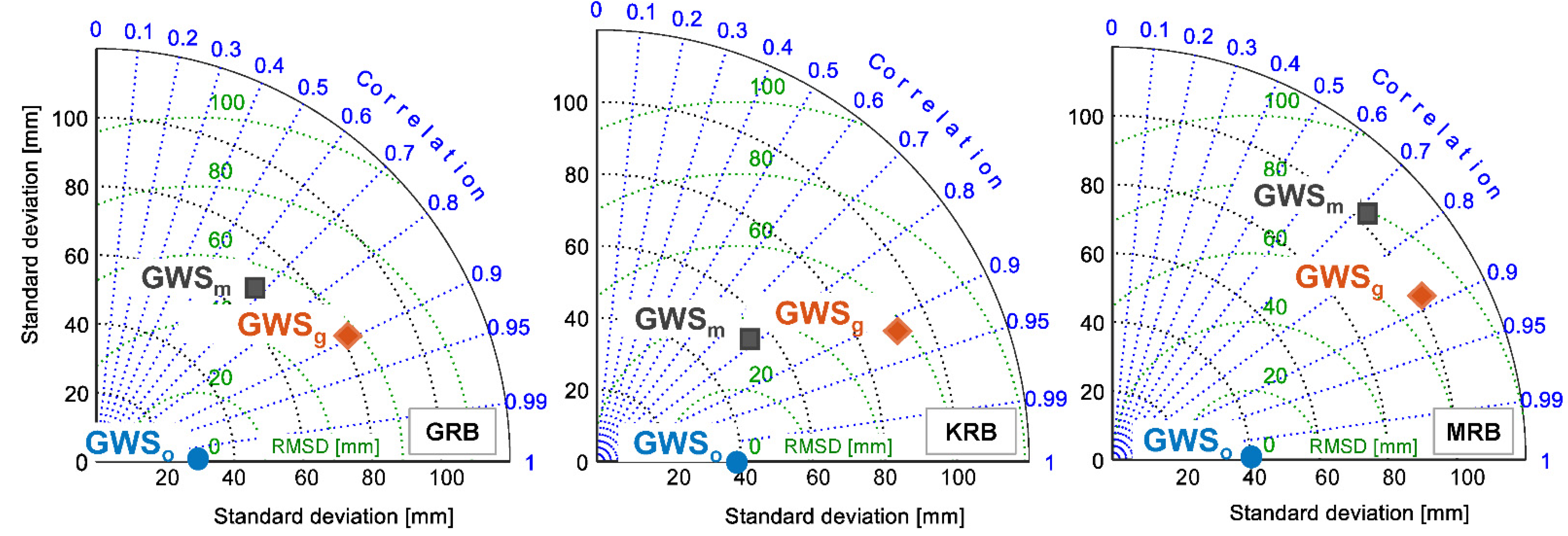
3.1. Multidecadal Trends in WSCs

The long-term linear trends in monthly ${\mathrm{LWS}}_{\mathrm{m}}$ from January 1980 to December 2014 were quantified as 0.56 mm yr⁻¹, 0.46 mm yr⁻¹, and 0.26 mm yr⁻¹, which correspond to the trends in an equivalent volume of 6.13 km³ yr⁻¹, 4.10 km³ yr⁻¹, and 1.29 km³ yr⁻¹ for GRB, KRB, and MRB, respectively. Despite stable linear trends in ${\mathrm{LWS}}_{\mathrm{m}}$, all three river basins exhibit a high inter-annual variability, which can primarily be explained by the precipitation. When compared with the ${\mathrm{LWS}}_{\mathrm{g}}$, ${\mathrm{LWS}}_{\mathrm{m}}$ underestimates both the declining and rising water storage during dry and wet periods, respectively, from April 2002 to December 2014, which is consistent with the findings reported by [24,42]. Nonlinear trends estimated by means of the HP filter reveal that, in general, KRB experienced stable dynamics of ${\mathrm{LWS}}_{\mathrm{m}}$ and its constituent components (${\mathrm{SMS}}_{\mathrm{m}}$, ${\mathrm{GWS}}_{\mathrm{m}}$) except for the extremely dry years of 1987 and 2003–2004 (Figure 3). GRB and MRB revealed almost similar dynamics of the various WSCs, albeit with higher amplitudes in MRB. ${\mathrm{LWS}}_{\mathrm{m}}$ showed a phase lag and amplitude difference from ${\mathrm{SMS}}_{\mathrm{m}}$ and ${\mathrm{GWS}}_{\mathrm{m}}$, which are attributed to the fact that ${\mathrm{LWS}}_{\mathrm{m}}$ combines all the WSCs, and hence the slower response of subsurface systems contributes to the existing lag, particularly that of ${\mathrm{GWS}}_{\mathrm{m}}$. Precipitation attains a maximum value in July (in GRB and KRB) or August (in MRB). ${\mathrm{SMS}}_{\mathrm{m}}$ and ${\mathrm{GWS}}_{\mathrm{m}}$ lag with a lag of 2–3 months from precipitation because of the natural process of recharge and other inherent vadose zone processes. ${\mathrm{SMS}}_{\mathrm{m}}$ showed similar dynamics in all three basins despite high variabilities in precipitation, particularly in MRB (Figure 3). ${\mathrm{LWS}}_{\mathrm{m}}$ responds strongly to the precipitation during the monsoon season (July–October), primarily following the ${\mathrm{GWS}}_{\mathrm{m}}$ dynamics as ascertained by the deseasonalized WSCs (Figure S2). The decline in ${\mathrm{GWS}}_{\mathrm{m}}$ and hence in ${\mathrm{LWS}}_{\mathrm{m}}$ during the nonmonsoon season (November–June) can be attributed to the combined impact of groundwater withdrawals for irrigation to the Rabi crops, basinal outflow, and evapotranspiration losses. Moreover, analyses of the deseasonalized and segregated WSCs revealed that the groundwater is the significant contributor to the ${\mathrm{LWS}}_{\mathrm{m}}$ during both depletion and recovery times with dominant effects of the South Asian summer monsoon (Supplementary Section S8). The comparatively slower response of GW fluctuations to hydrological fluxes (precipitation and evapotranspiration) than the near-surface WSCs imposes further stress on the replenishable limits of the groundwater withdrawals [30,43].

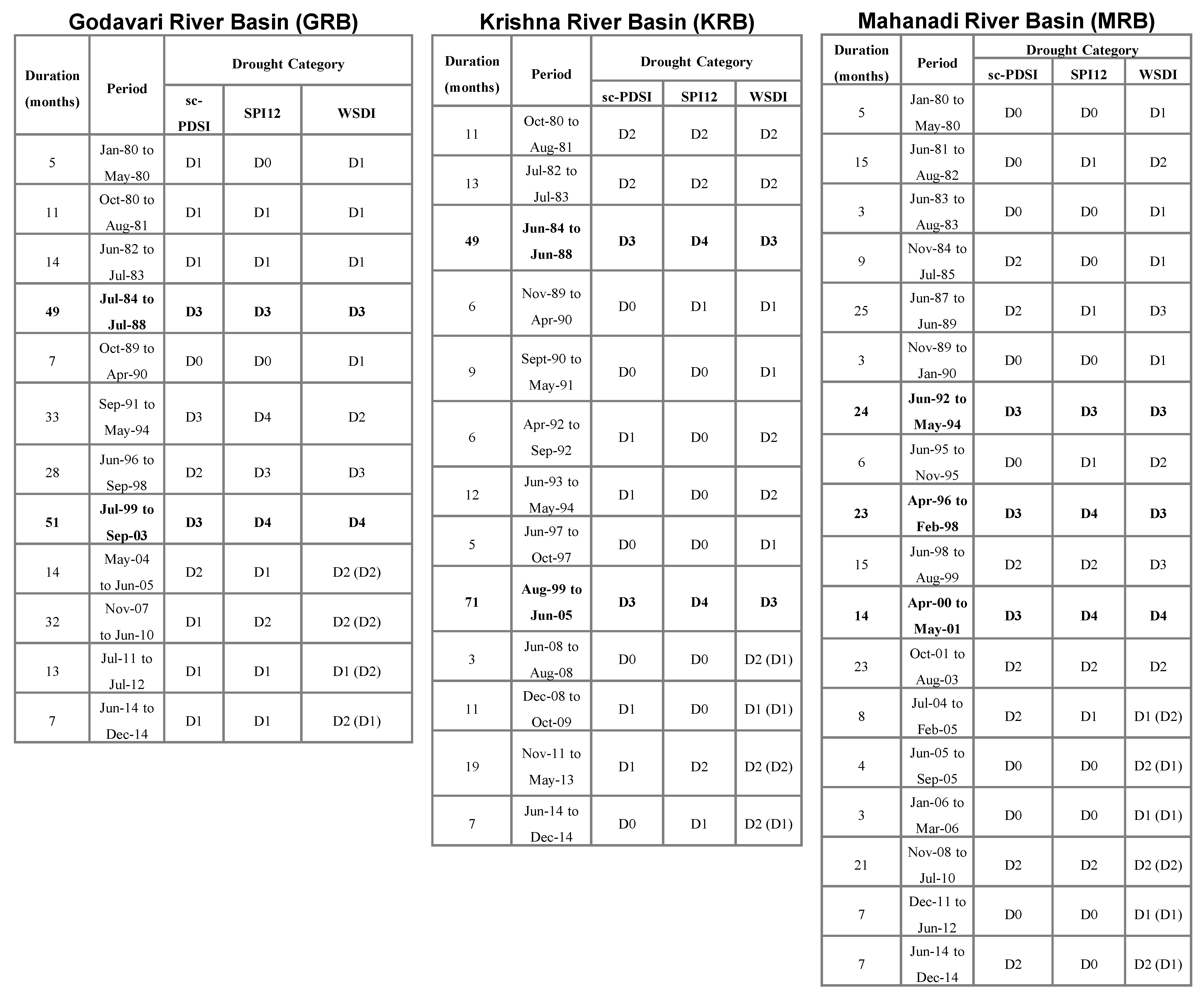
3.2. Estimation of Drought Severity and Recovery Time

From January 1980 to December 2014, Peninsular India has faced significant meteorological and agricultural droughts during 1987, 1997, 2002 [44], 2004, 2009, and 2015. LWSD has signatures of all these droughts, but a distinct behavior was observed in GWSD (e.g., no groundwater deficit condition was detected in 1997 and 2009 in the KRB). Assessment of the intra-annual distribution of the monthly deficit events reveals that July is the most drought-prone month for LWSD for all three basins (Figure S3), while for GWSD, there is no fixed pattern. To further quantify the fluctuations in ${\mathrm{LWS}}_{\mathrm{m}}$ or ${\mathrm{GWS}}_{\mathrm{m}}$, we calculated the monthly water storage deficits (WSD) for all basins based on Equation (1) (Figure S4). A period showing a continuous deficit (negative value of WSD) for equal to or more than three months was classified as a single drought event, while the deficit of one or two months can be explained by the precipitation variability or any other localized activities in the region. The results reveal that all three basins witness a variable number of droughts with varying severity where MRB experienced a comparatively larger number of deficit events (LWSD/GWSD events; 18/15) compared to GRB (12/12) and KRB (13/12) (Figure S4). The longest and the most severe LWSD event was quantified in KRB from August 1999 to June 2005 (71 months) with a total and average severity of −2220 and −32 mm months, respectively, and the highest LWSD of −104 mm in September 2002. Regarding GWSD, GRB experienced the longest and the most severe deficit spanning 84 months (July 1999 to June 2006) with a total and average severity of −3085 and −36 mm months, respectively, and a maximum GWSD of −120 mm in September 2004 (Figure 4 and Figure S5). Minimum recovery time analysis estimates the time taken to reach the normal water storage (${\mathrm{LWS}}_{\mathrm{m}}$ or ${\mathrm{GWS}}_{\mathrm{m}}$) conditions in the basin. The fastest recovery corresponds to 7.2/6.3, 7.3/8.17, and 8.4/4.75 months (October 2002/September 2004, September 2002/December 2004, and October 2000/July 2002, respectively, for LWSD/GWSD) (Figure 4). The cumulative time needed for the recovery of GWSD reaches as high as 161 months (July 1999 to June 2006), 185 months (November 2000 to June 2005), and 43 months (April 2009 to April 2011) for GRB, KRB, and MRB, respectively (Figure 4).

The occurrence of multi-year groundwater deficits as revealed by the currently employed storage-based approach and the accumulated recovery time of as long as 15 years indicates that the groundwater systems are highly vulnerable to the joint influence of the hydrometeorological variability (e.g., rainfall) and human influences. Therefore, there is a need for maintaining a resilient subsurface system that can continue to support local people in the study area even when severe and frequent meteorological droughts occur. Furthermore, the multidecadal analysis enables us to assess the intra-seasonal variations of GW in the region thoroughly. For example, the GWSD continued through the wet season, indicating that although there may be sufficient surface water, the deficiency in GW is still continuing, albeit invisible. The majority of the water storage deficits do not attain peaks from April to June even when there is low precipitation, which is because the minimum anomaly of ${\mathrm{LWS}}_{\mathrm{m}}$ (largest negative LWSD) is quite stable over the study period, while the maximum anomaly changes a lot from year to year, mainly depending on the amount of net precipitation flux. This storage-based assessment of groundwater droughts offers the potential to develop efficient drought-monitoring and -forecasting systems under sustainable and conjugative water utilities. Moreover, the different patterns of frequency and severity of groundwater droughts among the basins suggest employing the season-independent site-specific drought mitigation approach.

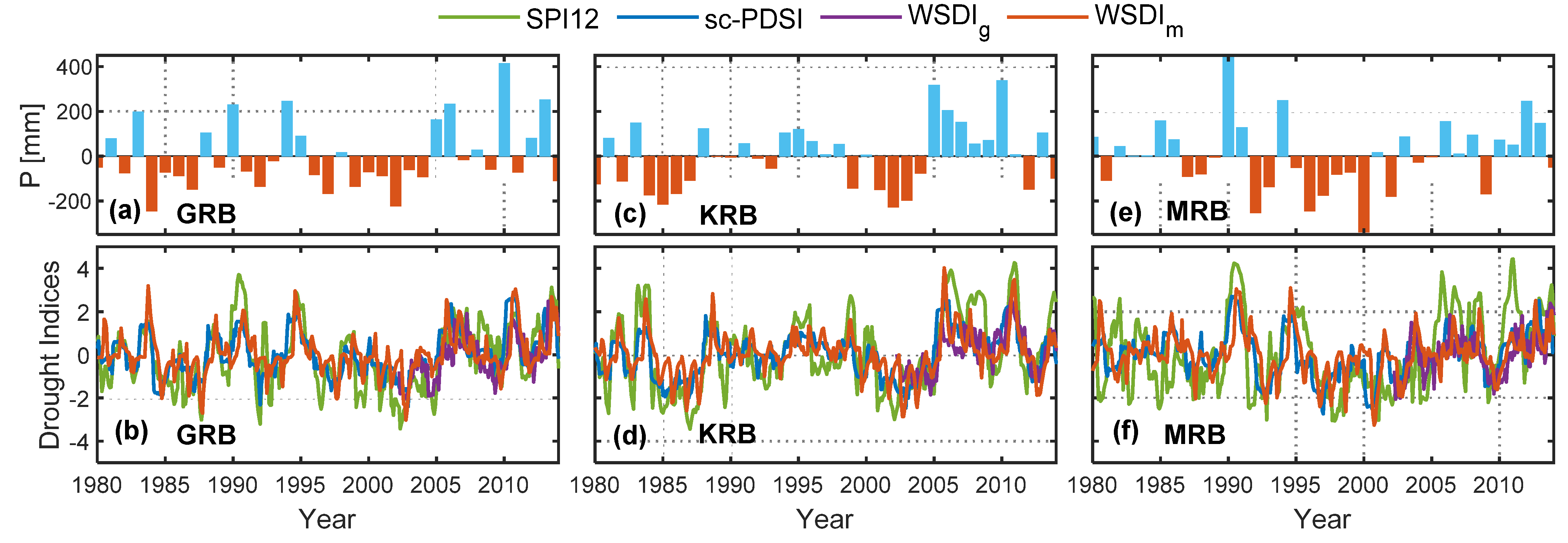
3.3. How Well Does WSDI Compare with sc-PDSI and SPI12?

The long-term general behavior of ${\mathrm{WSDI}}_{\mathrm{m}}$ agreed well with sc-PDSI and SPI12 in all three basins (Figure 5). All the indices are linearly correlated (Pearson correlation r > 0) and show similar monotonic behavior (Spearman’s rho $\rho$> 0). Both r and $\rho$ are higher between ${\mathrm{WSDI}}_{\mathrm{m}}$ and sc-PDSI than those between ${\mathrm{WSDI}}_{\mathrm{m}}$ and SPI12 for all the basins (Table S1). This behavior is because the calculation of sc-PDSI, unlike SPI12, involves both the meteorological and hydrological variables and takes the regional water balance into account, while ${\mathrm{WSDI}}_{\mathrm{m}}$ includes the integrated water storage. The linear correlation, as well as the rank correlation amongst the drought indices, is stronger in the case of the GRB and KRB as compared to the MRB primarily attributable to the comparatively smaller basin area of MRB where the lateral fluxes may have induced uncertainties in the estimation of various WSCs, which subsequently propagated in the calculation of the different indices.

Interestingly, all peaks in the severe or extreme drought events (classified as per Table S2) based on ${\mathrm{WSDI}}_{\mathrm{m}}$ occurred in September–October when the study region received above-average rainfall and witnessed minimal groundwater extraction as a result of the monsoon. This behavior of peak deficits ascertains that the area has suffered from a prolonged deficiency in integrated water storage. Although the monsoon rainfall may have quickly replenished the (near)-surface water deficiency, the water fluxes’ cumulative balance could not be attained, primarily due to the prolonged persistence of GWSD. On the contrary, the peak deficits of water storage in the events of less severity and small duration occur throughout the year with no characteristic pattern. This behavior can be explained by the individual or combined effects of localized heterogeneous rainfall events, climatic shifts in particular years, and perturbations due to human activities (groundwater abstractions) in the specific region.

In general, the classification of the drought events with high severity agreed well amongst the three drought indices than the events with less severity (Figure A1). For example, the longest drought event, which lasted for 71 months (~6 years) in KRB, was classified as a severe drought (D3) by both sc-PDSI and ${\mathrm{WSDI}}_{\mathrm{m}}$ and as extreme drought (D4) by SPI12 (Figure A1). Likewise, almost all the major drought events differed in their classification by a maximum of one level among the three indices, and the maximum difference in the levels was two for other drought events. Overall, given the spatiotemporal continuity, the integrated response from natural climate variability or anthropogenic intervention, and a simple but robust approach that is free from any physical model uncertainties, ${\mathrm{WSDI}}_{\mathrm{m}}$ outperformed the conventional indices, with few instances of minor variations amongst various indices essentially arising from the definition of ${\mathrm{WSDI}}_{\mathrm{m}}$. A more detailed and explicit discussion on the observed variations among various indices is shown below.

${\mathrm{WSDI}}_{\mathrm{m}}$ does not capture the local short-term drought events that might have occurred due to the climatic variations. For instance, the drought event from September 1991 to May 1994 in the GRB is classified as extreme (D4) based on SPI12, which is based only on precipitation but is classified as moderate (D2) by ${\mathrm{WSDI}}_{\mathrm{m}}$ (Table S4). During this period, the rainfall was consistently decreasing compared to the baseline (Figure S2), but the overall deficit in the region could not be much more severe, thus making the difference in drought levels identified by two indices. The event severity was maximum for the LWSD events categorized as severe to extreme (defined as per Table S3), with two events in each of the GRB and KRB and three events in the MRB (Table S4). The event severity of these events is −1570 mm months and −1614 mm months in the GRB, −1590 mm months and −2220 mm months in the KRB, and −1340 mm months, −1451 mm months, and −1137 mm months in the MRB (Figure S5, Table S4).

The drought event in MRB (April 2000 to May 2001) with the severity of −1135.25 mm months is classified as extreme drought (D4) based on ${\mathrm{WSDI}}_{\mathrm{m}}$ and SPI12 even though the severity is much smaller than other drought events categorized as D3 or D4 in the basins. For ${\mathrm{WSDI}}_{\mathrm{m}}$, this observation can be explained because the drought category is primarily dependent on the minimum water storage conditions and not on the severity of the event. For the SPI12 classification, the difference can partially be attributed to the varying scale and shape parameters of the gamma distribution with rainfall records and partially to the fact that SPI12 primarily depends on the 12-month averaging precipitation and not on the integrated water resources.

The larger fluctuation and amplitude with some sharp peaks and troughs in SPI12 than in sc-PDSI and ${\mathrm{WSDI}}_{\mathrm{m}}$ can be attributed directly to the monthly variations in rainfall. The similar time variations in sc-PDSI and ${\mathrm{WSDI}}_{\mathrm{m}}$ are mainly attributed to the subsurface hydrological processes with a dampened response, leading to a small difference in drought categories identified by the two indices. The inherent governing physical mechanisms and algorithms employed in each drought index result in the difference in the identified drought level. In calculating sc-PDSI and SPI12, the water fluxes within a limited soil depth and a single meteorological variable, i.e., precipitation, are, respectively, used, while some critical hydrological components are neglected, leading to the biased evaluation of the hydrological fluxes. On the contrary, the actual drought conditions in a region are derived by more inclusive dynamics of the basin-scale hydrologic system. For the Indian scenario, where the extraction and voluminous use of groundwater are highest in the world with an annual rate of 230 km³, ${\mathrm{WSDI}}_{\mathrm{m}}$ seems to be better than the traditional indices in predicting and assessing the drought events’ severity. Therefore, ${\mathrm{WSDI}}_{\mathrm{m}}$ is considered to outperform the conventional indices for manifold reasons: (a) it integrates the surface and subsurface water storages and thus portrays a holistic picture of water storage dynamics; (b) it includes more straightforward and transparent numerical and statistical computations; (c) it represents the near real-time and most accurate measurements over the study region, which is not valid in the case of indices derived from the data from the limited hydro-meteorological stations; (d) it depicts the continuity of the temporal dynamics of the water storage.

Further, ${\mathrm{WSDI}}_{\mathrm{g}}$ is in good agreement with ${\mathrm{WSDI}}_{\mathrm{m}}$ from April 2002 to December 2014 (Figure 5). Statistical comparison between the two indices showed a strong correlation (r = 0.66, 0.74, and 0.62 for GRB, KRB, and MRB, respectively). Moreover, ${\mathrm{WSDI}}_{\mathrm{g}}$ showed a higher correlation than ${\mathrm{WSDI}}_{\mathrm{m}}$ with sc-PDSI and SPI12 in all the basins (except for SPI12 in MRB), because GRACE records the real-time data and is free from any atmospheric or model uncertainties in ${\mathrm{LWS}}_{\mathrm{m}}$ induced by the model’s physical structure. A maximum of one level of difference can be seen in the drought category of the two indices (${\mathrm{WSDI}}_{\mathrm{g}}$ and ${\mathrm{WSDI}}_{\mathrm{m}}$) for the drought events post-April 2002 (Figure A1), which can be attributed to the coarse resolution of GRACE data and uncertainties in climate forcing parameters, and limited adequacy of the model structure. The qualitative behavior of ${\mathrm{WSDI}}_{\mathrm{g}}$ and the traditional indices, i.e., sc-PDSI and SPI12, are similar to the results reported by [2].

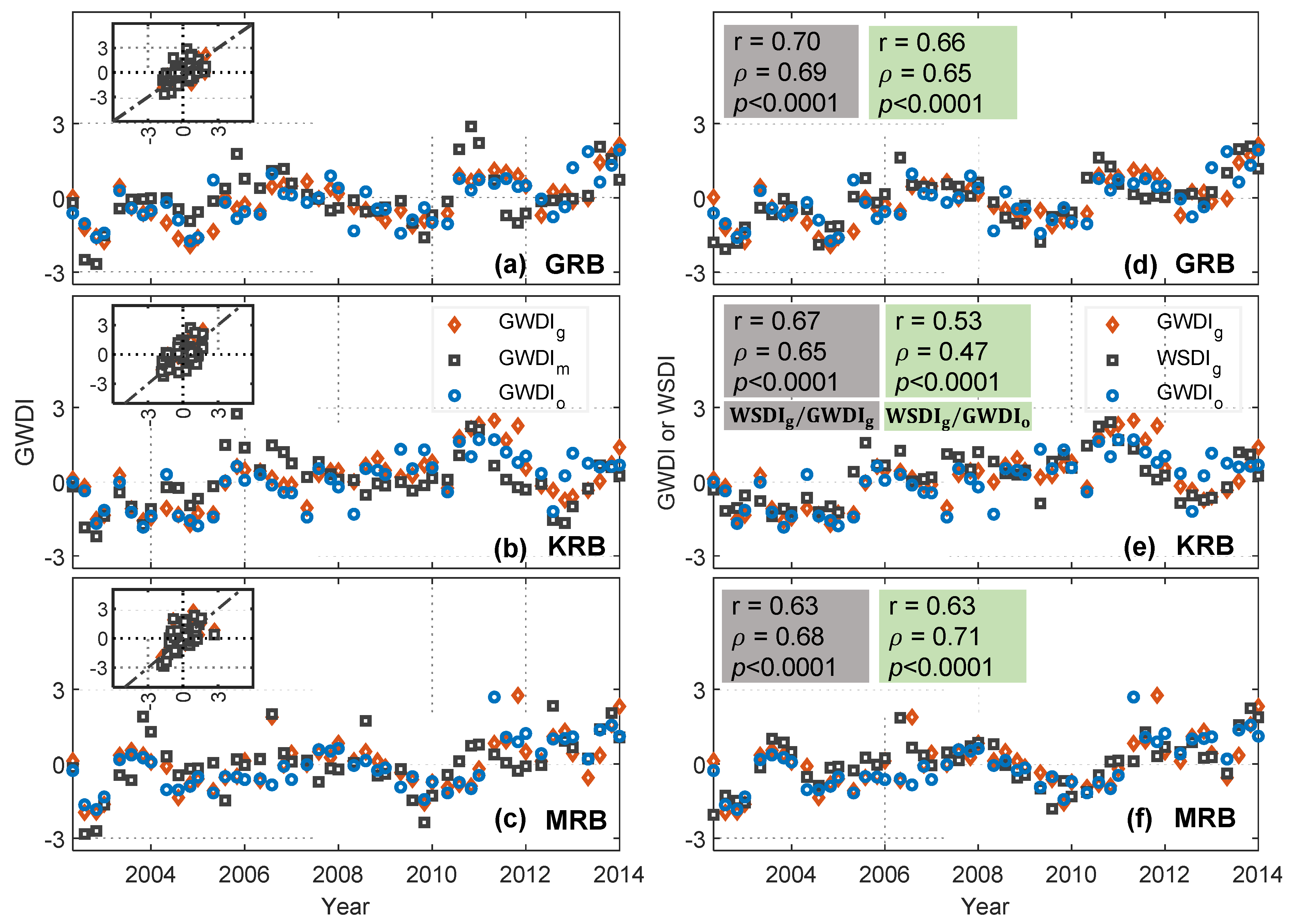
3.4. Characterizing GWDI and Potential of WSDI as a Proxy for GWDI

For characterizing the temporal variations in GW and validating the model output, we compared the three groundwater storage anomaly series, viz., ${\mathrm{GWS}}_{\mathrm{m}}$ (modeled), ${\mathrm{GWS}}_{\mathrm{g}}$ (GRACE-derived), and ${\mathrm{GWS}}_{\mathrm{o}}$ (in situ observed), in terms of the standard deviation (representing the amplitude of their variations), correlation, and centered root-mean-square (RMS) difference (Figure A2). Both ${\mathrm{GWS}}_{\mathrm{m}}$ and ${\mathrm{GWS}}_{\mathrm{g}}$ have large standard deviations (${\mathrm{GWS}}_{\mathrm{g}}$: 81.18, 90.9, and 101.90 mm; ${\mathrm{GWS}}_{\mathrm{m}}$: 68.04, 54.36, and 103.32 mm) compared to ${\mathrm{GWS}}_{\mathrm{o}}$ (28.91, 38.81, and 40.23 mm) for all three basins. Further, to assess the potential of ${\mathrm{GWDI}}_{\mathrm{m}}$, we inter-compared three normalized groundwater drought indices to quantify the groundwater drought conditions (Supplementary Section S7). Qualitatively, all three indices show similar phase variations. ${\mathrm{GWDI}}_{\mathrm{m}}$ compared favorably well with ${\mathrm{GWDI}}_{\mathrm{o}}$ showing a similar seasonal dynamic with maxima and minima occurring in August (monsoon season) or November (post-monsoon season), and in May (pre-monsoon or summer season), respectively (Figure 6). However, sporadically high and sharp amplitude differences are observed probably because of the loss of GW to deep aquifers, short but heavy rainfall events, the influence of direct intrusion of floodwater to the open wells, lateral inflow and outflow to the groundwater, and the response lag compared to the GRACE real-time records [29,45,46]. ${\mathrm{GWS}}_{\mathrm{o}}$ and ${\mathrm{GWS}}_{\mathrm{g}}$ records (with data processing uncertainties and partly biased by the inherent uncertainties in ${\mathrm{SMS}}_{\mathrm{m}}$) represent the actual groundwater storage, and hence the derived indices are close to each other and smoother than ${\mathrm{GWDI}}_{\mathrm{m}}$. Furthermore, the scatter plots indicate a good agreement between ${\mathrm{GWDI}}_{\mathrm{g}}$ and ${\mathrm{GWDI}}_{\mathrm{o}}$ (almost following the 1:1 line) in all three basins, while ${\mathrm{GWDI}}_{\mathrm{m}}$ shows more diffused plots against ${\mathrm{GWDI}}_{\mathrm{o}}$ (Figure 6a–c inset). ${\mathrm{GWDI}}_{\mathrm{o}}$ has a strong correlation (r = 0.75–0.80, p < 0.0001) with ${\mathrm{GWDI}}_{\mathrm{g}}$ and moderate correlation (r ~ 0.50, p < 0.001) with ${\mathrm{GWDI}}_{\mathrm{m}}$, attributed to the reason that the changes in ${\mathrm{GWS}}_{\mathrm{m}}$ estimated by the dynamic equilibrium of the five-module setup of PCR-GLOBWB are not as direct as those captured by GRACE and in situ observations.

Lastly, the good agreement of ${\mathrm{WSDI}}_{\mathrm{g}}$ with ${\mathrm{GWDI}}_{\mathrm{g}}$ (r = 0.63–0.70, $\rho$= 0.65–0.69, p < 0.0001) and ${\mathrm{GWDI}}_{\mathrm{o}}$ (r = 0.53–0.66, $\rho$= 0.47–0.71, p < 0.0001) highlights the potential of ${\mathrm{WSDI}}_{\mathrm{g}}$ as a proxy indicator to assess the groundwater drought situation in the region (Figure 6). Furthermore, the lagged correlation between ${\mathrm{WSDI}}_{\mathrm{g}}$ and ${\mathrm{GWDI}}_{\mathrm{g}}$ is maximum with r = 0.82, 0.84, and 0.78 at a lag of one month. Hence, we infer that the ${\mathrm{WSDI}}_{\mathrm{g}}$ can be used to monitor the groundwater (with a lead time of one month, i.e., LWS at ith month can be used to represent GWS at i+1th month), as well as the land water storage-based drought conditions, in real-time using the GRACE satellite observations, thus eliminating the need for any complex model simulations.

3.5. Inferences for the Sustainable Groundwater Utilities in the Study Region

The high impact of the South Asian monsoon rainfall on the regional groundwater resources and the recovery time analysis highlight the need for employing a conjunctive water management strategy in the region. In India, similar to other areas of high dependency on groundwater, the groundwater withdrawals increase during the drought years to meet the various water demands. After drought years, the near-surface components recover quickly by the seasonal increase in the influx (i.e., net precipitation), but the groundwater storage retains the deficits for a longer time. We believe that the decadal dynamics of the groundwater storage and the analysis of severity and recovery time of various groundwater drought events will help foster the discussion for the sustainable use of the prevailing groundwater in the region. For policy recommendation, we believe that constituting a Liaison Committee of multiple ministries and stakeholders for recognition and promoting the sound hydrological cycles and formulation and implementation of revitalization plans will lead toward a water-sustainable area because these members are expected to be inefficient while working independently.

To ensure freshwater availability across the country and reduce the farmer’s dependency on the highly heterogeneous monsoon, India’s National Water Development Agency has undertaken the Interlinking of Rivers (ILR) project. Out of the 16 links under the Peninsular Indian region, the Mahanadi Godavari link is the first and critical link of the nine link systems of Mahanadi-Godavari-Krishna-Pennar-Cauvery-Vaigai-Gundar of the National Perspective Plan under the ILR project. The southern peninsular component will contribute to an estimated 30 million hectares of irrigation by surface water [47]. Apart from aiding various auxiliary sectors such as pollution control, navigation, and power generation, the ILR project will reduce the stress on the prevailing groundwater resources and mitigate the impacts of hydrological extremes by ensuring homogeneous accessibility and equity in water distribution.

3.6. Limitations of the Study

Various WSC simulations by the global hydrological models have been reported to underestimate the trends [24,30], and therefore, one could argue about using the outputs from multiple models. It should be noted that the assessment of the variability in output among different global hydrologic models is out of the scope of the current manuscript. We chose the PCR-GLOBWB model just for demonstration purposes of how well we can understand the dynamics and variability of land storage and its constituent components beyond the GRACE period and subsequently assess the capability of land water storage (whether ${\mathrm{LWS}}_{\mathrm{g}}$ or ${\mathrm{LWS}}_{\mathrm{m}}$) to depict the near-real-time groundwater situation in the region.

Regarding the global hydrological model, it should be calibrated with the ground data, wherever available (e.g., soil moisture [48], discharge data [49]), and the performance should be further analyzed statistically for the study region in consideration. In addition, the applicability of the model as an auxiliary data source for GRACE-based water storage estimation can further be characterized either using more recent satellite datasets of soil moisture (e.g., SMAP; Soil Moisture Active Passive), land water storage (e.g., Swarm [50]), among others. Additionally, the advancements toward hyper-resolution global water resource modeling and improved methods of satellite gravimetry may further enhance our understanding of the various regional and global hydrological systems.

4. Conclusions

Herein, we analyzed the multidecadal (1980–2014) trends (linear and nonlinear) in various WSCs, dynamics of deseasonalized water storage deficits, and drought characterization in terms of magnitude, duration, severity, and recovery time, with an explicit focus on groundwater.

Key findings of the study are summarized below:

• The PCR-GLOBWB model is largely suitable for quantifying individual and integrated WSCs in a region and subsequent decadal droughts assessment for the period beyond GRACE records, especially prior to April 2002.
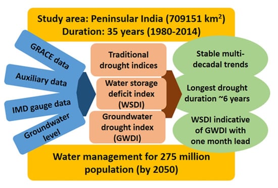
• Contrary to the near-surface storage components, the commonly invisible GWS showed a slow but persistent response (longest deficit period spanning ~6 years) to the seasonal variations of the hydrological fluxes and remained the major contributor to LWS.
• The observed behavior of occurrence of all of the severe-to-extreme drought events highlights the region’s vulnerability to drought conditions even in the monsoon season. This behavior, combined with the recovery time analysis, will help understand the temporal propagation of GW deficits and take precautionary measures to prevent overexploitation.
• WSDI holistically characterizes the drought intensity in a particular region owing to its independence from the geographical area. It enables us to quantify the integrated water deficit below average conditions, unlike the conventional indices where only a few hydrometeorological components are included, and therefore, it is useful in efficient drought monitoring.
• ${\mathrm{WSDI}}_{\mathrm{g}}$ agrees favorably well (similar dynamics and high correlation (r = 0.53–0.70)) with the ${\mathrm{GWDI}}_{\mathrm{g}}$ and ${\mathrm{GWDI}}_{\mathrm{o}}$, highlighting the potential of the remotely sensed WSDI as a quick proxy of groundwater with a lead time of one month, thus eliminating the need for the groundwater storage simulations in data-scarce river basins globally, which is otherwise quite complex and may inevitably possess high uncertainties.

In areas such as India, where there is a current lack of a real-time integrated drought monitoring framework for reference, the present study will help better understand long-term systemic changes in the hydrological system. Our study will provide the blueprint for the comprehensive characterization of drought events using WSDI, and the current approach can subsequently be utilized to understand the basin-scale dynamics of the water resources and subsequent effective and efficient water resources management and policymaking, especially in the data-scarce or data-limited river basins globally.

References

1. Du, L.; Tian, Q.; Yu, T.; Meng, Q.; Jancsó, T.; Udvardy, P.; Huang, Y. A Comprehensive Drought Monitoring Method Integrating Modis and Trmm Data. Int. J. Appl. Earth Obs. Geoinf. 2013, 23, 245–253. [Google Scholar] [CrossRef]
2. Sun, Z.; Zhu, X.; Pan, Y.; Zhang, J.; Liu, X. Drought Evaluation Using the Grace Terrestrial Water Storage Deficit over the Yangtze River Basin, China. Sci. Total Environ. 2018, 634, 727–738. [Google Scholar] [CrossRef] [PubMed]
3. Jacobi, J.; Perrone, D.; Duncan, L.L.; Hornberger, G. A Tool for Calculating the Palmer Drought Indices. Water Resour. Res. 2013, 49, 6086–6089. [Google Scholar] [CrossRef]
4. Abhishek; Kinouchi, T.; Sayama, T. A Comprehensive Assessment of Water Storage Dynamics and Hydroclimatic Extremes in the Chao Phraya River Basin during 2002–2020. J. Hydrol. 2021, 603, 126868. [Google Scholar] [CrossRef]
5. Schreiner-Mcgraw, A.P.; Ajami, H. Delayed Response of Groundwater to Multi-Year Meteorological Droughts in the Absence of Anthropogenic Management. J. Hydrol. 2021, 603, 126917. [Google Scholar] [CrossRef]
6. Dai, A. Increasing Drought under Global Warming in Observations and Models. Nat. Clim. Chang. 2013, 3, 52–58, Erratum in Nat. Clim. Chang. 2013, 3, 171. [Google Scholar] [CrossRef]
7. Trenberth, K.E.; Dai, A.; Van Der Schrier, G.; Jones, P.D.; Barichivich, J.; Briffa, K.R.; Sheffield, J. Global Warming and Changes in Drought. Nat. Clim. Chang. 2014, 4, 17–22. [Google Scholar] [CrossRef]
8. Mishra, A.K.; Singh, V.P. A Review of Drought Concepts. J. Hydrol. 2010, 391, 202–216. [Google Scholar] [CrossRef]
9. Thomas, B.F.; Famiglietti, J.S.; Landerer, F.W.; Wiese, D.N.; Molotch, N.P.; Argus, D.F. Grace Groundwater Drought Index: Evaluation of California Central Valley Groundwater Drought. Remote Sens. Environ. 2017, 198, 384–392. [Google Scholar] [CrossRef]
10. Bloomfield, J.P.; Marchant, B.P.; Bricker, S.H.; Morgan, R.B. Regional Analysis of Groundwater Droughts using Hydrograph Classification. Hydrol. Earth Syst. Sci. 2015, 19, 4327–4344. [Google Scholar] [CrossRef] [Green Version]
11. Li, B.; Rodell, M.; Kumar, S.; Beaudoing, H.K.; Getirana, A.; Zaitchik, B.F.; De Goncalves, L.G.; Cossetin, C.; Bhanja, S.; Mukherjee, A.; et al. Global Grace Data Assimilation for Groundwater and Drought Monitoring: Advances and Challenges. Water Resour. Res. 2019, 55, 7564–7586. [Google Scholar] [CrossRef] [Green Version]
12. Scanlon, B.R.; Faunt, C.C.; Longuevergne, L.; Reedy, R.C.; Alley, W.M.; Mcguire, V.L.; Mcmahon, P.B. Groundwater Depletion and Sustainability of Irrigation in the US High Plains and Central Valley. Proc. Natl. Acad. Sci. USA 2012, 109, 9320–9325. [Google Scholar] [CrossRef] [PubMed] [Green Version]
13. Famiglietti, J.S.; Lo, M.; Ho, S.L.; Bethune, J.; Anderson, K.J.; Syed, T.H.; Swenson, S.C.; De Linage, C.R.; Rodell, M. Satellites Measure Recent Rates of Groundwater Depletion in California’s Central Valley. Geophys. Res. Lett. 2011, 38, L03403. [Google Scholar] [CrossRef] [Green Version]
14. Famiglietti, J.S. The Global Groundwater Crisis. Nat. Clim. Chang. 2014, 4, 945–948. [Google Scholar] [CrossRef]
15. Richey, A.S.; Thomas, B.F.; Lo, M.-H.; Reager, J.T.; Famiglietti, J.S.; Voss, K.; Swenson, S.; Rodell, M. Quantifying Renewable Groundwater Stress With Grace. Water Resour. Res. 2015, 51, 5217–5238. [Google Scholar] [CrossRef] [PubMed]
16. Siebert, S.; Burke, J.; Faures, J.M.; Frenken, K.; Hoogeveen, J.; Döll, P.; Portmann, F.T. Groundwater Use for Irrigation—A Global Inventory. Hydrol. Earth Syst. Sci. 2010, 14, 1863–1880. [Google Scholar] [CrossRef] [Green Version]
17. Zaveri, E.; Grogan, D.S.; Fisher-Vanden, K.; Frolking, S.; Lammers, R.B.; Wrenn, D.H.; Prusevich, A.; Nicholas, R.E. Invisible Water, Visible Impact: Groundwater Use and Indian Agriculture under Climate Change. Environ. Res. Lett. 2016, 11, 084005. [Google Scholar] [CrossRef] [Green Version]
18. Worldbank India Groundwater: A Valuable but Diminishing Resource. Available online: http://www.worldbank.org/en/news/feature/2012/03/06/india-groundwater-critical-diminishing (accessed on 15 October 2021).
19. Chindarkar, N.; Grafton, R.Q. India’s Depleting Groundwater: When Science Meets Policy. Asia Pac. Policy Stud. 2019, 6, 108–124. [Google Scholar] [CrossRef]
20. CGWB. Dynamic Ground Water Dynamic Ground Water Resources of India; CGWB: New Delhi, India, 2014.
21. Suhag, R. Overview Of Groundwater in India; Working Papers id:9504; eSocialSciences: Vashi, India, 2016. [Google Scholar]
22. Li, B.; Rodell, M. Evaluation of a Model-Based Groundwater Drought Indicator in the Conterminous U.S. J. Hydrol. 2015, 526, 78–88. [Google Scholar] [CrossRef] [Green Version]
23. Rodell, M.; Famiglietti, J.S.; Wiese, D.N.; Reager, J.T.; Beaudoing, H.K.; Landerer, F.W.; Lo, M.-H. Emerging Trends in Global Freshwater Availability. Nature 2018, 557, 651–659. [Google Scholar] [CrossRef]
24. Scanlon, B.R.; Zhang, Z.; Save, H.; Sun, A.Y.; Schmied, H.M.; Van Beek, L.P.H.; Wiese, D.N.; Wada, Y.; Long, D.; Reedy, R.C.; et al. Global Models Underestimate Large Decadal Declining and Rising Water Storage Trends Relative to Grace Satellite Data. Proc. Natl. Acad. Sci. USA 2018, 115, E1080–E1089. [Google Scholar] [CrossRef] [PubMed] [Green Version]
25. Andrew, R.; Guan, H.; Batelaan, O. Estimation of Grace Water Storage Components by Temporal Decomposition. J. Hydrol. 2017, 552, 341–350. [Google Scholar] [CrossRef] [Green Version]
26. Jing, W.; Zhao, X.; Yao, L.; Jiang, H.; Xu, J.; Yang, J.; Li, Y. Variations in Terrestrial Water Storage in the Lancang-Mekong River Basin from Grace Solutions and Land Surface Model. J. Hydrol. 2020, 580, 124258. [Google Scholar] [CrossRef]
27. Chen, J.; Tapley, B.; Rodell, M.; Seo, K.-W.; Wilson, C.; Scanlon, B.R.; Pokhrel, Y. Basin-Scale River Runoff Estimation from Grace Gravity Satellites, Climate Models, and In Situ Observations: A Case Study in the Amazon Basin. Water Resour. Res. 2020, 56, E2020wr028032. [Google Scholar] [CrossRef]
28. Scanlon, B.R.; Zhang, Z.; Reedy, R.C.; Pool, D.R.; Save, H.; Long, D.; Chen, J.; Wolock, D.M.; Conway, B.D.; Winester, D. Hydrologic Implications of Grace Satellite Data in the Colorado River Basin. Water Resour. Res. 2015, 51, 9891–9903. [Google Scholar] [CrossRef]
29. Long, D.; Chen, X.; Scanlon, B.R.; Wada, Y.; Hong, Y.; Singh, V.P.; Chen, Y.; Wang, C.; Han, Z.; Yang, W. Have Grace Satellites Overestimated Groundwater Depletion in the Northwest India Aquifer? Sci. Rep. 2016, 6, 24398. [Google Scholar] [CrossRef]
30. Abhishek; Kinouchi, T. Synergetic Application of Grace Gravity Data, Global Hydrological Model, and In-Situ Observations to Quantify Water Storage Dynamics Over Peninsular India during 2002–2017. J. Hydrol. 2021, 596, 126069. [Google Scholar] [CrossRef]
31. Kumar, K.S.; Rathnam, E.V.; Sridhar, V. Tracking seasonal and monthly drought with grace-based terrestrial water storage assessments over major river basins in South India. Sci. Total Environ. 2021, 763, 142994. [Google Scholar] [CrossRef]
32. Goi Ground Water Year Book India 2016-Central Ground Water Board; Ministry of Water Resources; Government of India: Faridabad, India, 2017.
33. Census of India. Report of The Technical Group on Population Projections. 2019. Available online: https://nhm.gov.in/New_Updates_2018/Report_Population_Projection_2019.pdf (accessed on 28 July 2021).
34. CWC. Water and Related Statistics. Water Planning and Project Wing; Central Water Commission: New Delhi, India, 2020.
35. Pai, D.S.; Sridhar, L.; Rajeevan, M.; Sreejith, O.P.; Satbhai, N.S.; Mukhopadhyay, B. Development of a new high spatial resolution (0.25° × 0.25°) long period (1901–2010) daily gridded rainfall data set over india and its comparison with existing data sets over the region. Mausam 2014, 65, 1–18. [Google Scholar] [CrossRef]
36. Abhishek; Abolafia-Rosenzweig, R.; Kinouchi, T.; Ito, M. Water budget closure in the Upper Chao Phraya River basin, Thailand using multisource data. Remote Sens. 2022, 14, 173. [Google Scholar] [CrossRef]
37. Sakumura, C.; Bettadpur, S.; Bruinsma, S. Ensemble prediction and intercomparison analysis of grace time-variable gravity field models. Geophys. Res. Lett. 2014, 41, 1389–1397. [Google Scholar] [CrossRef]
38. Hodrick, R.J.; Prescott, E.C. Postwar U.S. Business Cycles: An Empirical Investigation. J. Money Crédit Bank. 1997, 29, 1–16. [Google Scholar] [CrossRef]
39. Thomas, A.C.; Reager, J.T.; Famiglietti, J.S.; Rodell, M. A grace-based water storage deficit approach for hydrological drought characterization. Geophys. Res. Lett. 2014, 41, 1537–1545. [Google Scholar] [CrossRef] [Green Version]
40. Dai, A.; Trenberth, K.E.; Qian, T. A global dataset of palmer drought severity index for 1870–2002: Relationship with soil moisture and effects of surface warming. J. Hydrometeorol. 2004, 5, 1117–1130. [Google Scholar] [CrossRef]
41. Mckee, T.B.; Doesken, N.J.; Kleist, J. The relationship of drought frequency and duration to time scales. In Proceedings of the 8th Conference on Applied Climatology, Hot Springs, AR, USA, 16–18 November 1983. [Google Scholar]
42. Xu, L.; Chen, N.; Zhang, X.; Chen, Z. Spatiotemporal changes in China’s terrestrial water storage from grace satellites and its possible drivers. J. Geophys. Res. Atmos. 2019, 124, 11976–11993. [Google Scholar] [CrossRef]
43. Rodell, M.; Velicogna, I.; Famiglietti, J.S. Satellite-based estimates of groundwater depletion in India. Nature 2009, 460, 999–1002. [Google Scholar] [CrossRef] [Green Version]
44. Mallya, G.; Mishra, V.; Niyogi, D.; Tripathi, S.; Govindaraju, R.S. Trends and variability of droughts over the indian monsoon region. Weather Clim. Extrem. 2016, 12, 43–68. [Google Scholar] [CrossRef] [Green Version]
45. Rodell, M.; Chen, J.; Kato, H.; Famiglietti, J.S.; Nigro, J.; Wilson, C.R. estimating groundwater storage changes in the Mississippi river basin (USA) using grace. Hydrogeol. J. 2007, 15, 159–166. [Google Scholar] [CrossRef] [Green Version]
46. Panda, D.K.; Wahr, J. Spatiotemporal Evolution of Water Storage Changes in India from the Updated Grace-Derived Gravity Records. Water Resour. Res. 2016, 52, 135–149. [Google Scholar] [CrossRef] [Green Version]
47. Department of Water Resources; Mojs, J.S. Department of Water Resources, River Development & Ganga Rejuvenation, Government of India. Available online: http://jalshakti-dowr.gov.in/ (accessed on 28 August 2021).
48. López, P.L.; Sutanudjaja, E.H.; Schellekens, J.; Sterk, G.; Bierkens, M.F.P. Calibration of A large-scale hydrological model using satellite-based soil moisture and evapotranspiration products. Hydrol. Earth Syst. Sci. 2017, 21, 3125–3144. [Google Scholar] [CrossRef] [Green Version]
49. Sutanudjaja, E.H.; Van Beek, L.P.H.; De Jong, S.M.; Van Geer, F.C.; Bierkens, M.F.P. Calibrating a large-extent high-resolution coupled groundwater-land surface model using soil moisture and discharge data. Water Resour. Res. 2014, 50, 687–705. [Google Scholar] [CrossRef]
50. Richter, H.M.P.; Lück, C.; Klos, A.; Sideris, M.G.; Rangelova, E.; Kusche, J. Reconstructing grace-type time-variable gravity from the swarm satellites. Sci. Rep. 2021, 11, 1117. [Google Scholar] [CrossRef] [PubMed]
Figure 1. Study area specifications. (a) Godavari, Krishna, and Mahanadi river basins (GRB, KRB, and MRB, respectively) selected for the current study. The grid points corresponding to the IMD (India Meteorological Department) gridded precipitation data and the groundwater well locations are also shown by filled red diamonds and filled black circles, respectively. (b) Basin-wide estimates of total replenishable groundwater resources (km3), geographical area (km2), and annual precipitation (mm) from January 1980 to December 2014. Further specifications of the study basins are listed in Section 2.1.
Remotesensing 14 01486 g001
Figure 2. Summary of the research flow. A schematic showing the outline of data sources, data types, methods used, and analysis performed in the study.
Remotesensing 14 01486 g002
Figure 3. Nonlinear trends and seasonal variability. (ac) Nonlinear (Hodrick–Prescott) trends in the anomaly time series of precipitation (P), modeled soil moisture storage ( SMS m ), modeled groundwater storage ( GWS m ), and modeled land water storage ( LWS m ) from January 1980 to December 2014 and GRACE-derived LWS ( LWS g ) from April 2002 to December 2014 for GRB (a), KRB (b), and MRB (c). (df) Box-whisker plots of P, SMS m , GWS m , and LWS m anomalies in GRB (d), KRB (e), and MRB (f) from January 1980 to December 2014. The values of all the variables are shown in equivalent water depth (mm). The horizontal lines within the boxes represent the median value, the extent of the box signifies the 25th–75th percentile (inter-quartile) range of the respective data, and the lower and upper whisker limits represent the ±1 standard deviation of the individual time series.
Remotesensing 14 01486 g003
Figure 4. Comparison of drought severity and recovery time in GWS m and LWS m . (ac) Average event severity for the drought (deficit) events identified in LWS m and GWS m for GRB (a), KRB (b), and MRB (c) from January 1980 to December 2014. Maximum LWS m deficits (LWSD) and GWS m deficits (GWSD) are also shown by the stem plots. (df) Minimum recovery time corresponding to the monthly deficits (both LWSD and GWSD) during the study period.
Remotesensing 14 01486 g004
Figure 5. Comparison of WSDI with traditional drought indices. Anomaly time series of precipitation and various drought indices (sc-PDSI, SPI12, WSDI m , and WSDI g for GRB (a,b), KRB (c,d), and MRB (e,f), respectively).
Remotesensing 14 01486 g005
Figure 6. Comparison of various GWDIs. (ac) Groundwater drought indices derived from GRACE-based GWSA ( GWDI g ), from GWS m -based GWSA ( GWDI m ), and calculated using the in situ well data ( GWDI o ) for the GRB (a), KRB (b), and MRB (c) from May 2002 to January 2014. The GWDI time series are denoted four times a year (January, May, August, and November) when the observed GWS records are available. Scatter plots of GWDI g and GWDI m with GWDI o for all three river basins are also shown in the insets. The 1:1 lines are also shown with dashed black lines. (df) Comparison of WSDI g with GWDI g and GWDI o for the GRB (d), KRB (e), and MRB (f). Pearson correlation coefficient (r), Spearman rho ( ρ ), and p-values for WSDI g and GWDI g (grey boxes), and WSDI g and GWDI o (light green boxes) are also shown for the three river basins.
Remotesensing 14 01486 g006