A Scalable and Accurate De-Snowing Algorithm for LiDAR Point Clouds in Winter

Abstract

Accurate and efficient environmental awareness is a fundamental capability of autonomous driving technology and the real-time data collected by sensors offer autonomous vehicles an intuitive impression of their environment. Unfortunately, the ambient noise caused by varying weather conditions immediately affects the ability of autonomous vehicles to accurately understand their environment and its expected impact. In recent years, researchers have improved the environmental perception capabilities of simultaneous localization and mapping (SLAM), object detection and tracking, semantic segmentation and panoptic segmentation, but relatively few studies have focused on enhancing environmental perception capabilities in adverse weather conditions, such as rain, snow and fog. To enhance the environmental perception of autonomous vehicles in adverse weather, we developed a dynamic filtering method called Dynamic Distance–Intensity Outlier Removal (DDIOR), which integrates the distance and intensity of points based on the systematic and accurate analysis of LiDAR point cloud data characteristics in snowy weather. Experiments on the publicly available WADS dataset (Winter Adverse Driving dataSet) showed that our method can efficiently remove snow noise while fully preserving the detailed features of the environment.

1. Introduction

Autonomous driving technology is a novel technology that is being rapidly developed by interdisciplinary researchers. Manufacturers, such as Waymo, Tesla and Xpeng, have reportedly achieved Level 2+ (partial automation) autonomous driving; in addition, the mass production of L3 (conditional automation) autonomous vehicles is imminent and L4 (high automation) autonomous vehicles will soon be released. Despite the revolutionary success of autonomous vehicles to date, safe driving in adverse weather, such as rain, snow and fog, remains an unavoidable and urgent technical problem. To advance the continued development of autonomous driving technology, many researchers are studying environmental perception in different weather conditions. By studying the effects of different weather conditions on sensors and data, numerous sensor combinations for autonomous vehicles have been analyzed and summarized. As the eyes of autonomous vehicles, sensors are the key to environmental perception and cognition. Keisuke et al. [1] analyzed the performance of visual sensors, LiDAR and millimeter wave radar (MWR) technologies, which are commonly used in autonomous vehicles under different weather conditions, and concluded that the visual sensors were the most susceptible to weather, as shown in

Table 1. The influences of sensors on adverse weather conditions. The conclusions in this table come from [1].

Sensors	Sun Glare	Rain	Fog	Snow
LiDAR		Reflectivity degradation Reduction in measuring Shape change due to splash	Reflectivity degradation Reduction in measuring	Noise due to snow Road surface occlusion
MWR		Reduction in measuring	Reduction in measuring	Noise due to snow
Camera	Whiteout of objects	Visibility degradation	Visibility degradation	Visibility degradation Road surface occlusion

. Targeted data de-noising studies have been conducted by analyzing the characteristics of multisource sensor data under different weather conditions, predominantly with de-raining and de-fogging [2,3] while fewer de-snowing studies have been performed. Considering the more extensive applicability of LiDAR in different weather conditions compared to visual sensors, this study focused on enhancing the environmental perception of autonomous vehicles in winter by point cloud data de-noising.

The Sensible 4 bus, a Finnish autonomous bus that recently underwent a public test in snowy conditions, is the latest achievement of research into the operation of autonomous vehicles in winter. Even human drivers are cautious when driving in snowy conditions, so there is no doubt that adverse weather conditions have delayed the development of autonomous driving technology and that snowy conditions pose a serious challenge to the implementation of this technology [4]. The challenges are manifold: first, snowflakes adhere to sensors, thereby inhibiting the detection of signals and reducing the detection range; second, snowflakes in their solid state tend to collect and form solid obstacles or are distributed in high densities around the sensors; third, snowflakes adhere to the surfaces of various environmental elements, such as vehicles, road signs and buildings, resulting in low intensity values being collected by the sensors; fourth, snowfall may cause snow to accumulate on the road, which may change the drivable area and affect the accuracy of route planning. From the perspective of environmental perception, the impact of snow on the acquisition of LiDAR data is intuitively reflected in the point cloud; hence, dealing with the snow noise in the point cloud is a key factor in determining the robustness and accuracy of environmental perception. Several representative LiDAR de-snowing methods have emerged that are based on the characteristics of snowflakes, including: the filtering method, which treats snow noise as outliers and is combined with statistical analysis to remove snow noise [5]; intensity filtering algorithms that remove snow noise based on its low intensity [6]; a dynamic radius filtering method designed to remove snow noise based on the characteristics of the LiDAR point cloud (the LiDAR point cloud is denser at closer distances, i.e., the number of points decreases as the distance increases) [7]; and the CNN-based de-snowing method (however, this method is limited by the dataset and thus, its generalization needs to be improved) [8]. Based on these research findings, we systematically analyzed the characteristics of LiDAR point cloud data under snowy conditions, clarified the distribution pattern of the point cloud and developed a dynamic filter that integrates distance and intensity. The experimental results from the WADS dataset [5] fully demonstrate the effectiveness of our method. The main contributions of this study are described as follows:

(1)

The characteristics of LiDAR point cloud data under snowy conditions were systematically analyzed in terms of distance, intensity and data percentage, providing solid support for subsequent studies;

(2)

Given the characteristics of point cloud data, a dynamic filter that integrates distance and intensity was developed. This method has thresholds that are dynamically adjustable to fully preserve environmental characteristics that are based on the accurate removal of snow noise. Evaluation experiments on the WADS dataset demonstrated the excellent performance of our method.

The remainder of this paper is organized as follows. Section 2 presents a review of related work. Section 3 provides the details of our method. The experimental results from the WADS dataset are presented in Section 4. Finally, a brief conclusion and discussion are presented in Section 5.

2. Related Work

Point cloud filtering is essential to ensure high-quality and highly available data. In this section, the principal point cloud filtering methods are presented, with a focus on LiDAR point cloud filtering methods in snowy conditions.

Mainstream point cloud filtering methods can be divided into the following five categories [9]: (1) statistics-based filtering methods, such as point cloud filtering based on principal component analysis [10] or Bayesian estimation [11]; (2) neighborhood-based filtering methods, which achieve point cloud filtering by using the neighborhood information of each point to calculate the similarity between points and of which bilateral filtering is a representative method [12]; (3) projection-based filtering methods, which can be interpreted as the projection of the point cloud in multiple perspectives [13] or the use of different projection strategies [14] to achieve point cloud filtering; (4) voxel-based filtering methods, which rasterize the point cloud and filter the points within the voxel that then serve as the basic unit [15]; (5) other filtering methods, including the signal processing-based filtering method, the partial differential-based filtering method and filtering methods that integrate multiple methods [16].

Snow noise is a type of noise encountered in outdoor environments that results in distinctive outlier noise clusters; consequently, it is difficult to remove by means of conventional filtering methods for surface noise points or point cloud filtering methods that are applicable to indoor environments. Based on the characteristics of snow noise, there are three principal types of filtering methods that can be applied to LiDAR point clouds collected under snowy conditions, as introduced below.

(1)

Statistics-based Snow Noise Filtering Methods

Statistical outlier removal (SOR) and radius outlier removal (ROR) are the most conventional point cloud noise filtering methods [15]. SOR uses a k-d tree to calculate the average distance of the k-nearest neighbors of each point, determines the filtering radius threshold based on the average distance and then rejects the points for which the nearest neighbor distance is greater than the threshold and keeps the points for which the nearest neighbor distance is within the threshold. ROR also calculates the average distance of the k-nearest neighbors of each point based on the k-d tree to determine the threshold of the filtering radius and then rejects the points for which the number of nearest neighbors is less than the threshold and retains the points for which the number of nearest neighbors is more than the threshold. When snow noise points are filtered, there are significant limitations in terms of the filtering rate and accuracy; for instance, the “near is dense, far is sparse” characteristics of the LiDAR point cloud causes both filtering methods to discard long-range environmental feature points.

The fixed filter radius form is difficult to apply to LiDAR point clouds, especially for point cloud data with snow noise. The presence of snow noise makes the average distance calculated by the k-d tree shorter than the average distance calculated for the point clouds that are free of ambient noise and as a result, the filter directly discards points that are slightly farther away. From a filtering accuracy perspective and to address the limitations imposed by a fixed filtering radius, dynamic radius outlier removal (DROR) [7] dynamically varies the filtering radius based on the point distance to admit more distant environmental feature points and performs well in light snow. Dynamic statistical outlier removal (DSOR) performs better in de-snowing at long distances than DROR while also obtaining better recall results and being applicable to more severe snow conditions; however, its de-snowing accuracy is slightly lower than that of DROR. Fast cluster statistical outlier removal (FCSOR) [17] accelerates the filtering process by voxel subsampling and parallel computation, but it only focuses on improving the filtering rate without improving the accuracy.

Yao et al. considered both the filtering rate and time, adopted principal component analysis to reduce the point cloud to two dimensions and used the DBSCAN algorithm for clustering to remove the sparse areas [18]; however, the accuracy of this method when dealing with snow noise needs to be further improved.

(2)

Intensity-based Snow Noise Filtering Methods

Low-intensity outlier removal (LIOR) [6] filters snow noise based on the judgment that the intensity of snow noise points is lower than the intensity of non-snow points over the same distance. The points below the intensity threshold are first screened and the prescreened potential snow noise points are then given a specified search radius to determine the number of nearest neighbors for each point; the points below the nearest neighbor threshold are judged to be snow noise points. LIOR integrates intensity-based prescreening and ROR, which significantly shortens the filtering time and improves the filtering accuracy. Dynamic light–intensity outlier removal (DIOR) [19], in contrast, integrates LIOR and DROR to further improve the filtering accuracy by dynamically adjusting the filtering radius.

(3)

Deep Learning-based Snow Noise Filtering Methods

WeatherNet [8], which uses LiLaNet [20] as the backbone network to reduce point cloud noise and produce a semantic segmentation network under different weather conditions and constructs training data by manually setting up the environment, is the most representative algorithm for this type of method. WeatherNet can reduce point cloud noise in certain weather conditions, such as rain, snow and fog, but its de-fogging performance is obviously better than its de-snowing and de-raining performance; furthermore, this method exhibits poor generalization because it is limited by datasets, which makes it difficult to popularize and use.

3. Materials and Methods

LiDAR point clouds vary with weather conditions; liquid substances (e.g., rain and fog) scatter laser signals, resulting in the sharp attenuation of the effective detection range, whereas solid substances (e.g., snow and dust) produce a large number of noise points in the point cloud. Obviously, there is no universal way to significantly enhance the environmental perception of autonomous vehicles in different weather conditions. Based on the specific weather conditions of snowy days, we systematically analyzed various characteristics of LiDAR point clouds, such as the distance, intensity and data distribution, and proposed a de-snowing algorithm that includes point cloud data prescreening, dynamic filtering and point cloud fusion. This section will introduce the data characteristics of LiDAR point clouds and the implementation process of the de-snowing algorithm in detail.

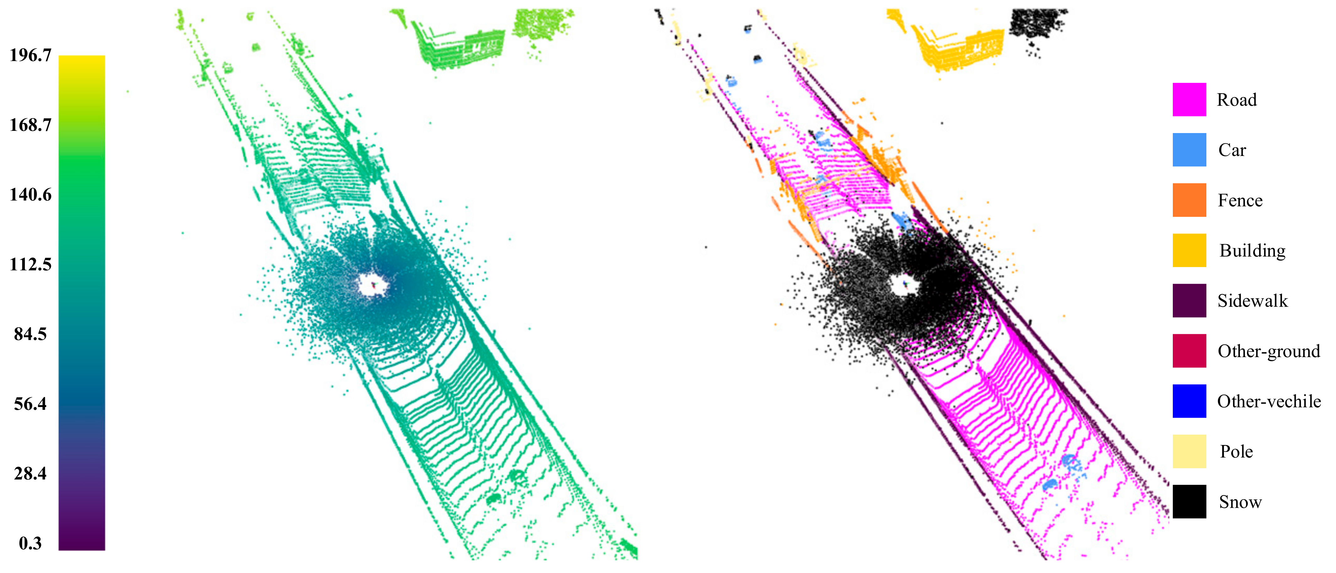
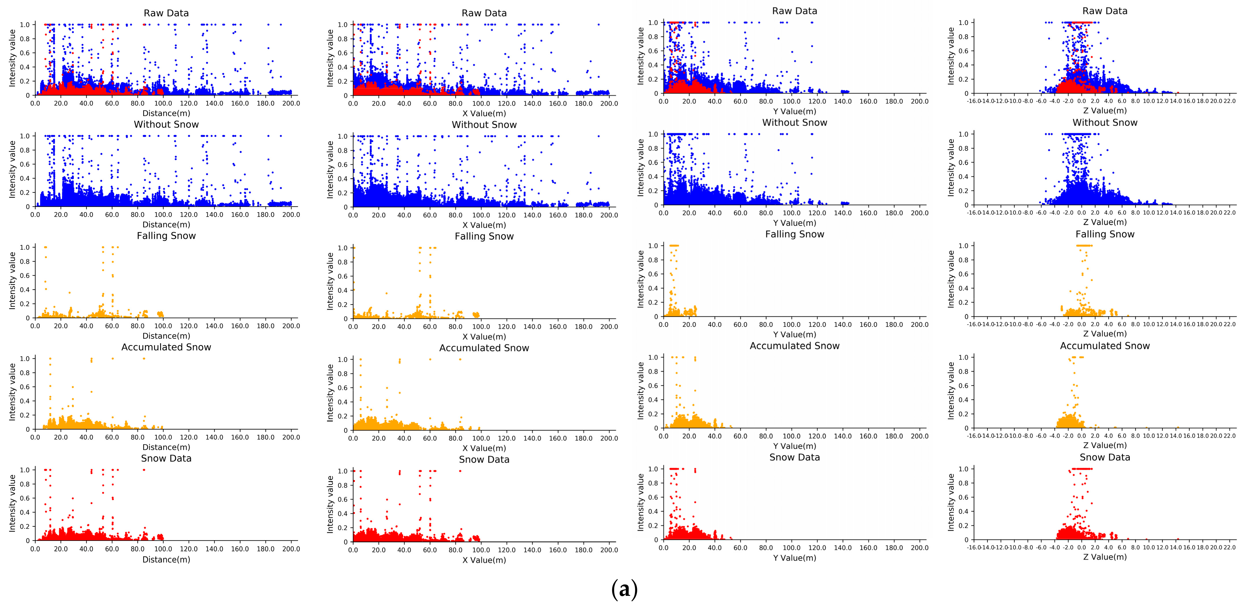
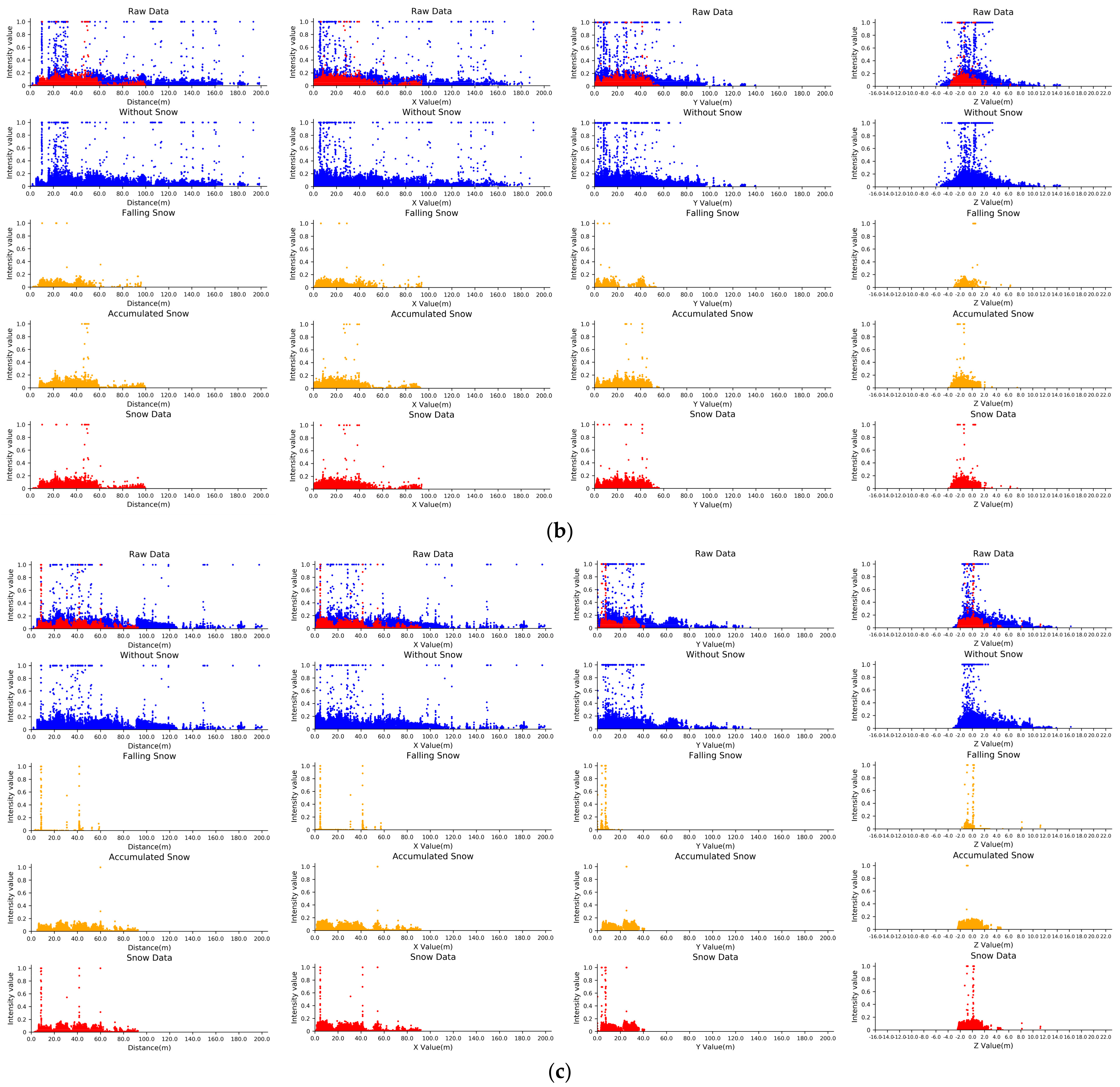
3.1. Characteristic Analysis of LiDAR Point Cloud Data Collected under Snowy Conditions

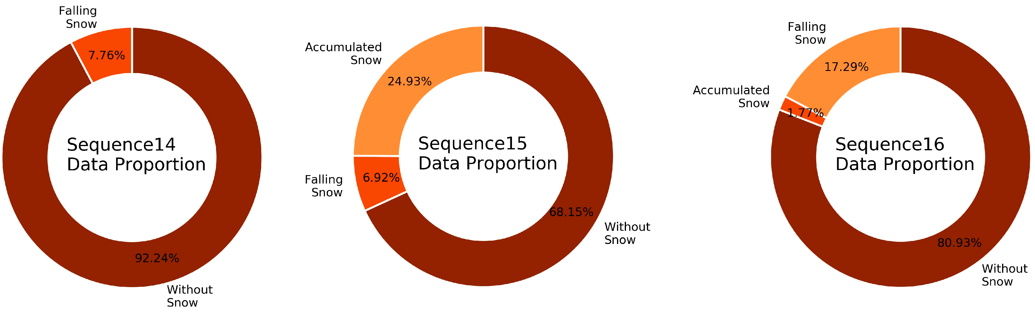
3.1.1. Basis of Data Analysis: The Dataset

The gradual construction of complete datasets has boosted the vigorous development of autonomous driving. The KITTI dataset [21], released in 2012, was the first multimodal dataset for autonomous driving tasks; this dataset was collected in clear weather with good visibility and is a common baseline dataset for evaluating environmental perception tasks, such as simultaneous localization and mapping (SLAM), multi-object detection and tracking, lane line detection and semantic segmentation. The 2016 Oxford RobotCar dataset [22] is a multimodal dataset designed for multiple identical scenarios that were acquired at different moments in different seasons; despite the data acquisition under different weather conditions, this dataset only contains a small amount of snow-related data and is primarily used in studies on SLAM and location recognition. With the rapid development of deep learning technology and the need for deep fine-grained environmental perception, datasets with fine annotation have emerged. The ApolloScape dataset [23], released in 2018, covers more weather conditions, such as cloudy and rainy days, accurately annotates vehicles in the environment and claims that snow data will be available as soon as possible. The Waymo dataset [24], nuScenes dataset [25] and SemanticKITTI dataset [26], all released in 2019, are mainstream autonomous driving (multimodal) datasets. The Waymo dataset presents entirely new challenges for three-dimensional (3D) object detection tasks in different weather conditions, but it includes no snow data. The nuScenes dataset and the SemanticKITTI dataset provide the point-wise semantic annotation of the data, which enables deeper and finer-grained environmental perception, such as semantic segmentation and panoptic segmentation, compared to 3D annotation scans and allows highly reliable data characterization based on accurate point-wise semantic annotation; however, neither dataset includes adverse weather conditions, such as rain, snow and fog. The SemanticKITTI dataset was derived from the point-wise semantic annotation of the LiDAR point cloud data from the KITTI dataset.

As seen from the development of the aforementioned datasets, the construction of datasets is moving toward all-weather data acquisition that covers different weather conditions and features fine point-wise data annotation. For snowy weather conditions, the DENSE dataset [27] and the Canadian Adverse Driving Conditions (CADC) dataset [28] were released successively in 2020. The DENSE dataset provides point cloud data with 3D annotated scans for rain, snow and fog and the CADC dataset provides point cloud data with 3D annotated scans for snowy weather; however, neither dataset provides fine point-wise annotation that allows for data analysis. The WADS dataset [5], released in 2021, includes over 26 TB of multimodal data on snowy days and approximately 7 GB of point cloud data containing 19 sequence sets with point-wise semantic annotation. This dataset adopts the 20 semantic categories delineated in the SemanticKITTI dataset and includes two additional categories: falling snow and accumulated snow. Compared to other snow-containing LiDAR point cloud data, the fine point-wise annotation of individual snowflakes in the WADS dataset fully reflects the environmental details, which facilitates data characterization, as shown in Figure 1.

We chose point-wise annotated data from the WADS dataset to characterize snow-containing point cloud data in terms of distance, intensity, data percentage and distribution. To ensure as much objectivity as possible in the data analysis and experimental validation, we divided the 19 available sequence sets (sequences 11–18, 20, 22–24, 26, 28, 30, 34–36 and 76) into a data analysis group (sequences 11–18 and 20), a method visualization group (sequence 22) and an experimental validation group (sequences 23–24, 26, 28, 30 and 34–36). We discarded sequence 76 because it contained only five scans.

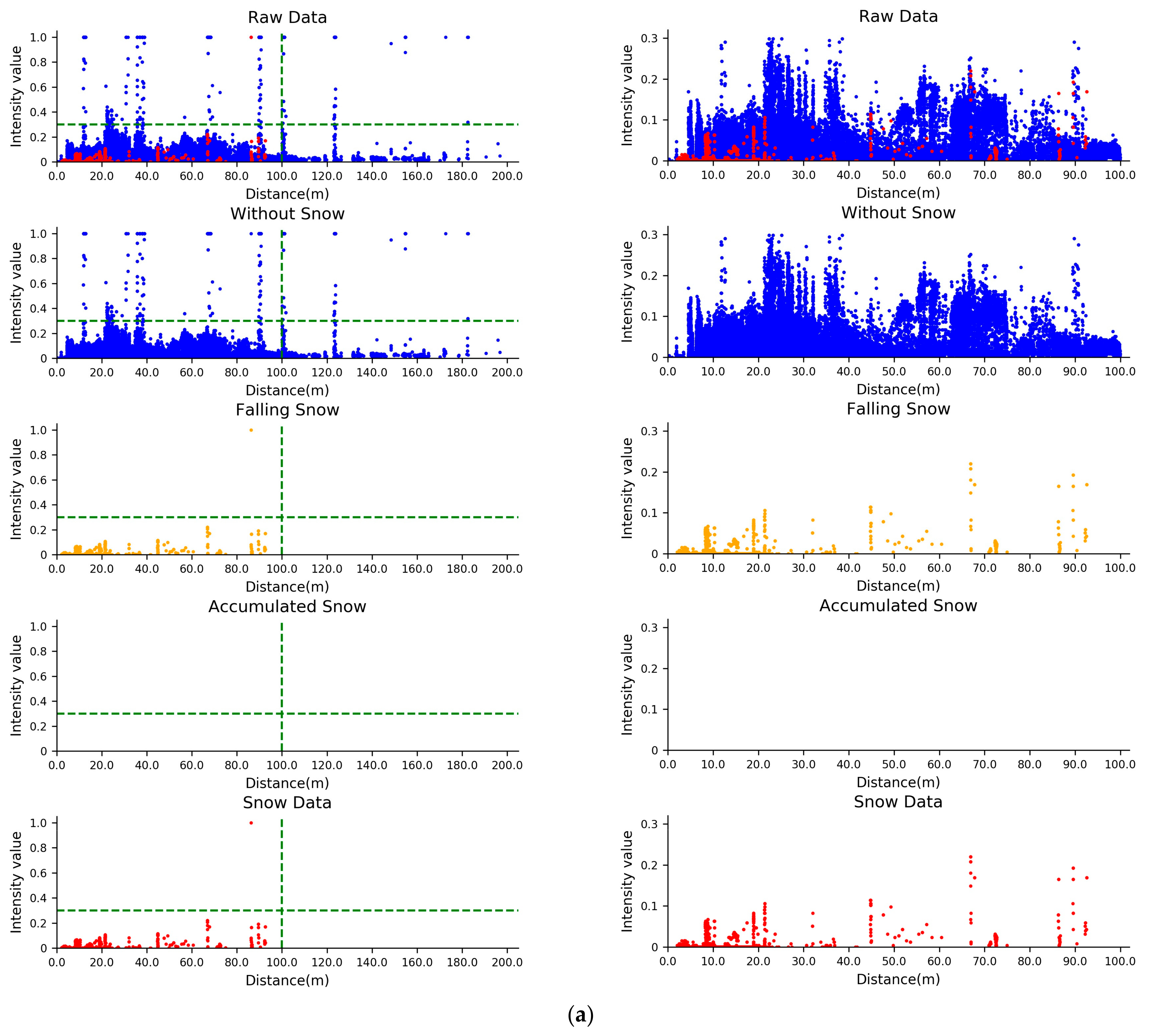
3.1.2. How Do Snowy Days Affect LiDAR Point Clouds?

From the point of view of data acquisition, for each scan of the point cloud that is collected by the LiDAR, the data of any point can be expressed as $P_n=\left(x,y,z,i\right)$, where $\left(x,y,z\right)$ represents the position coordinates of the point and $i$ denotes the intensity of the point; $r_n=P_n{}_2=\sqrt{x_n^2+y_n^2+z_n^2}$ is introduced to indicate the distance of the point from the sensor center. Therefore, the sensing information could be divided into two independent parts: $\left(x,y,z,r\right)$ and $i$ ($i$ is normalized). First, the 50th scan of sequences 11–13 was chosen to establish the correspondence between the $\left(\left|x\right|,\left|y\right|,z,r\right)$ and $i$ of snow noise points and non-snow points. The visualization is shown in Figure 2 and Figure 3. Figure 2 is composed of three subgraphs, which correspond to the statistics of the 50th scan of sequences 11–13 in turn. Each subgraph is the corresponding relationship between $\left(r,\left|x\right|,\left|y\right|,z\right)$ and $i$ from left to right. Among them, snow noise points are represented in red, non-snow points are represented in blue and falling snow and accumulated snow within snow noise points are represented in orange.

For comparison, we chose the 50th scan of sequences 01–03 in the SemanticKITTI dataset to establish the correspondence between $\left(r,\left|x\right|,\left|y\right|,z\right)$ and $i$ under sunny conditions. The corresponding visualizations are shown in Figure 3.

Figure 3 shows that the intensity values in a LiDAR point cloud decrease with increasing distance in clear weather conditions. From an intuitive comparison between Figure 2 and Figure 3, we can see that snow reduces the intensity of point cloud data.

After this initial analysis of the correspondence between distance and intensity, we selected the 60th scans from sequences 14–16 for use in a statistical analysis of the data percentages and distributions. A visualization of the statistics in terms of the percentage of snow noise points vs. non-snow points is presented in Figure 4, which shows that it is difficult to analyze the specific magnitudes of the weights of snow noise points from the data percentage perspective with natural factors as a force majeure.

With varying data percentages, the distributions of the data were further analyzed using distance as a statistical indicator. The statistical results are shown in

Table 2. Point cloud distribution in different distance intervals on sequence 14 of WADS.

	Distance	(0 m, 50 m)	(50 m, 100 m)	(100 m, 150 m)	(150 m, +∞)
Classification
Falling snow points		15,196	1195	0	0
Accumulated snow points		0	0	0	0
Non-snow points		184,045	9535	864	292

,

Table 3. Point cloud distribution in different distance intervals on sequence 15 of WADS.

	Distance	(0 m, 50 m)	(50 m, 100 m)	(100 m, 150 m)	(150 m, +∞)
Classification
Falling snow points		14,364	38	0	0
Accumulated snow points		49,610	2236	22	0
Non-snow points		123,333	16,600	1730	150

and

Table 4. Point cloud distribution in different distance intervals on sequence 16 of WADS.

	Distance	(0 m, 50 m)	(50 m, 100 m)	(100 m, 150 m)	(150 m, +∞)
Classification
Falling snow points		35,156	970	0	0
Accumulated snow points		3312	379	14	0
Non-snow points		156,717	11,435	793	127

(note that obtaining a suitable visualization was difficult due to the significant differences in weights between the different intervals; therefore, tables were selected for data presentation instead).

According to the tables, snow noise points tend to be concentrated within 100 m from the sensor and the shorter the distance, the greater the number of snow noise points. Thus, we can conclude that snow noise points are densely distributed around the sensor.

Following this clarification of the approximate effect that snowy weather has on the LiDAR point clouds, a more detailed data analysis was required to support the design of the de-snowing algorithm. We chose the data from the 70th scan of sequences 17, 18 and 20 for a two-pronged data analysis. First, the intensity values were divided equally into 10 intervals and the size of the data volume within each interval was counted separately, as shown in

Table 5. Point cloud distribution in different intensity intervals on sequence 17 of WADS.

	Intensity	(0, 0.1)	(0.1, 0.2)	(0.2, 0.3)	(0.3, 0.4)	(0.4, 0.5)	(0.5, 0.6)	(0.6, 0.7)	(0.7, 0.8)	(0.8, 0.9)	(0.9, 1.0)
Classification
Falling snow points		14,681	54	0	0	0	1	0	0	0	4
Accumulated snow points		28,277	344	28	19	8	5	2	0	6	34
Non-snow points		133,871	28,885	596	218	39	29	17	19	17	216

,

Table 6. Point cloud distribution in different intensity intervals on sequence 18 of WADS.

	Intensity	(0, 0.1)	(0.1, 0.2)	(0.2, 0.3)	(0.3, 0.4)	(0.4, 0.5)	(0.5, 0.6)	(0.6, 0.7)	(0.7, 0.8)	(0.8, 0.9)	(0.9, 1.0)
Classification
Falling snow points		14,737	0	1	0	0	0	0	0	0	0
Accumulated snow points		55,481	1021	12	5	5	0	0	0	1	27
Non-snow points		112,142	23,874	707	65	63	34	11	15	13	379

and

Table 7. Point cloud distribution in different intensity intervals on sequence 20 of WADS.

	Intensity	(0, 0.1)	(0.1, 0.2)	(0.2, 0.3)	(0.3, 0.4)	(0.4, 0.5)	(0.5, 0.6)	(0.6, 0.7)	(0.7, 0.8)	(0.8, 0.9)	(0.9, 1.0)
Classification
Falling snow points		35,592	261	4	2	7	2	5	3	3	44
Accumulated snow points		32,403	399	12	2	0	0	0	2	0	2
Non-snow points		110,280	1526	304	285	130	56	67	51	29	437

.

Second, with the intensity and distance values as indicators, the intensity values were divided equally into 10 intervals and the distances were divided into 20 intervals with detailed statistical distributions, as shown in

Table 8. Point cloud distribution in different distance and intensity intervals on sequence 17 of WADS.

	Distance	(0 m, 10 m)	(10 m, 20 m)	(20 m, 30 m)	(30 m, 40 m)	(40 m, 50 m)	(50 m, 60 m)	(60 m, 70 m)	(70 m, 80 m)	(80 m, 90 m)	(90 m, 100 m)	(100 m, 110 m)	(110 m, 120 m)	(120 m, 130 m)	(130 m, 140 m)	(140 m, 150 m)	(150 m, 160 m)	(160 m, 170 m)	(170 m, 180 m)	(180 m, 190 m)	$(190\mathbf{m},+\mathit{\infty })$
Classification & Intensity
Snow Noise Points	(0, 0.1)	14,735	16,913	5685	2780	1807	966	38	0	9	5	0	0	0	0	0	0	0	0	0	0
	(0.1, 0.2)	26	116	142	62	49	3	0	0	0	0	0	0	0	0	0	0	0	0	0	0
	(0.2, 0.3)	0	6	21	0	0	1	0	0	0	0	0	0	0	0	0	0	0	0	0	0
	(0.3, 0.4)	0	0	16	0	3	0	0	0	0	0	0	0	0	0	0	0	0	0	0	0
	(0.4, 0.5)	0	2	6	0	0	0	0	0	0	0	0	0	0	0	0	0	0	0	0	0
	(0.5, 0.6)	0	0	5	0	0	0	0	0	1	0	0	0	0	0	0	0	0	0	0	0
	(0.6, 0.7)	0	0	2	0	0	0	0	0	0	0	0	0	0	0	0	0	0	0	0	0
	(0.7, 0.8)	0	0	0	0	0	0	0	0	0	0	0	0	0	0	0	0	0	0	0	0
	(0.8, 0.9)	0	0	6	0	0	0	0	0	0	0	0	0	0	0	0	0	0	0	0	0
	(0.9, 1.0)	0	14	20	0	0	0	0	0	4	0	0	0	0	0	0	0	0	0	0	0
Non-Snow Points	(0, 0.1)	7420	60,310	25,987	18,140	11,848	4243	1872	1219	681	784	343	41	109	319	430	41	28	52	0	4
	(0.1, 0.2)	312	19,328	1774	1330	5529	355	27	17	59	93	4	0	0	51	4	0	1	1	0	0
	(0.2, 0.3)	0	394	155	14	13	10	0	2	0	4	0	0	2	0	0	2	0	0	0	0
	(0.3, 0.4)	0	155	30	28	1	4	0	0	0	0	0	0	0	0	0	0	0	0	0	0
	(0.4, 0.5)	0	17	16	4	0	1	1	0	0	0	0	0	0	0	0	0	0	0	0	0
	(0.5, 0.6)	0	9	8	0	2	2	0	2	0	2	0	0	2	0	0	1	0	0	0	1
	(0.6, 0.7)	0	11	2	4	0	0	0	0	0	0	0	0	0	0	0	0	0	0	0	0
	(0.7, 0.8)	0	6	2	2	0	3	0	2	0	0	0	2	0	0	2	0	0	0	0	0
	(0.8, 0.9)	0	6	4	2	2	0	0	0	0	0	0	0	1	0	0	2	0	0	0	0
	(0.9, 1.0)	0	152	22	16	2	10	0	0	0	7	0	0	0	0	1	1	0	5	0	0

,

Table 9. Point cloud distribution in different distance and intensity intervals on sequence 18 of WADS.

	Distance	(0 m, 10 m)	(10 m, 20 m)	(20 m, 30 m)	(30 m, 40 m)	(40 m, 50 m)	(50 m, 60 m)	(60 m, 70 m)	(70 m, 80 m)	(80 m, 90 m)	(90 m, 100 m)	(100 m, 110 m)	(110 m, 120 m)	(120 m, 130 m)	(130 m, 140 m)	(140 m, 150 m)	(150 m, 160 m)	(160 m, 170 m)	(170 m, 180 m)	(180 m, 190 m)	$(190\mathbf{m},+\mathit{\infty })$
Classification & Intensity
Snow Noise Points	(0, 0.1)	18,840	28,769	15,238	3905	1904	594	330	228	223	95	47	5	22	16	2	0	0	0	0	0
	(0.1, 0.2)	394	10	405	78	81	4	26	3	14	3	2	0	1	0	0	0	0	0	0	0
	(0.2, 0.3)	2	0	5	5	1	0	0	0	0	0	0	0	0	0	0	0	0	0	0	0
	(0.3, 0.4)	0	0	4	0	0	0	0	0	0	0	0	0	0	1	0	0	0	0	0	0
	(0.4, 0.5)	0	0	5	0	0	0	0	0	0	0	0	0	0	0	0	0	0	0	0	0
	(0.5, 0.6)	0	0	0	0	0	0	0	0	0	0	0	0	0	0	0	0	0	0	0	0
	(0.6, 0.7)	0	0	0	0	0	0	0	0	0	0	0	0	0	0	0	0	0	0	0	0
	(0.7, 0.8)	0	0	0	0	0	0	0	0	0	0	0	0	0	0	0	0	0	0	0	0
	(0.8, 0.9)	0	0	1	0	0	0	0	0	0	0	0	0	0	0	0	0	0	0	0	0
	(0.9, 1.0)	0	0	26	0	0	0	0	0	0	0	0	0	1	0	0	0	0	0	0	0
Non-Snow Points	(0, 0.1)	30,308	30,395	21,908	10,986	6482	4913	912	2206	1626	1247	617	40	4	78	41	4	353	14	0	8
	(0.1, 0.2)	8307	1568	4511	3982	3212	1195	35	436	390	217	7	0	0	14	0	0	0	0	0	0
	(0.2, 0.3)	31	2	390	229	38	0	5	2	0	2	6	2	0	0	0	0	0	0	0	0
	(0.3, 0.4)	18	0	18	20	8	0	1	0	0	0	0	0	0	0	0	0	0	0	0	0
	(0.4, 0.5)	16	0	12	17	7	3	3	4	0	1	0	0	0	0	0	0	0	0	0	0
	(0.5, 0.6)	2	0	8	13	6	3	2	0	0	0	0	0	0	0	0	0	0	0	0	0
	(0.6, 0.7)	4	0	1	6	0	0	0	0	0	0	0	0	0	0	0	0	0	0	0	0
	(0.7, 0.8)	0	0	4	8	3	0	0	0	0	0	0	0	0	0	0	0	0	0	0	0
	(0.8, 0.9)	0	0	4	6	0	3	0	0	0	0	0	0	0	0	0	0	0	0	0	0
	(0.9, 1.0)	0	2	131	115	82	18	10	21	0	0	0	0	0	0	0	0	0	0	0	0

and

Table 10. Point cloud distribution in different distance and intensity intervals on sequence 20 of WADS.

	Distance	(0 m, 10 m)	(10 m, 20 m)	(20 m, 30 m)	(30 m, 40 m)	(40 m, 50 m)	(50 m, 60 m)	(60 m, 70 m)	(70 m, 80 m)	(80 m, 90 m)	(90 m, 100 m)	(100 m, 110 m)	(110 m, 120 m)	(120 m, 130 m)	(130 m, 140 m)	(140 m, 150 m)	(150 m, 160 m)	(160 m, 170 m)	(170 m, 180 m)	(180 m, 190 m)	$(190\mathbf{m},+\mathit{\infty })$
Classification & Intensity
Snow Noise Points	(0, 0.1)	25,333	22,024	16,438	3145	730	145	69	29	64	18	0	0	0	0	0	0	0	0	0	0
	(0.1, 0.2)	4	248	351	37	5	4	0	2	9	0	0	0	0	0	0	0	0	0	0	0
	(0.2, 0.3)	0	2	8	6	0	0	0	0	0	0	0	0	0	0	0	0	0	0	0	0
	(0.3, 0.4)	0	2	0	0	0	0	0	0	0	2	0	0	0	0	0	0	0	0	0	0
	(0.4, 0.5)	0	0	0	5	0	0	0	0	2	0	0	0	0	0	0	0	0	0	0	0
	(0.5, 0.6)	0	0	0	2	0	0	0	0	0	0	0	0	0	0	0	0	0	0	0	0
	(0.6, 0.7)	0	0	0	4	0	0	0	1	0	0	0	0	0	0	0	0	0	0	0	0
	(0.7, 0.8)	0	2	0	1	2	0	0	0	0	0	0	0	0	0	0	0	0	0	0	0
	(0.8, 0.9)	0	2	0	1	0	0	0	0	0	0	0	0	0	0	0	0	0	0	0	0
	(0.9, 1.0)	0	10	0	8	9	0	0	0	4	15	0	0	0	0	0	0	0	0	0	0
Non-Snow Points	(0, 0.1)	8022	29,970	29,444	14,438	9784	4570	2263	1390	997	914	1170	2011	1135	2090	628	648	294	54	53	405
	(0.1, 0.2)	22	177	409	160	43	30	72	28	109	137	130	120	51	12	2	10	2	1	1	10
	(0.2, 0.3)	0	248	13	15	3	2	2	9	0	0	9	0	0	1	0	0	0	2	0	0
	(0.3, 0.4)	0	262	9	0	1	1	2	4	0	0	0	2	0	0	0	0	0	2	0	2
	(0.4, 0.5)	0	98	8	4	0	0	2	7	2	2	2	0	0	5	0	0	0	0	0	0
	(0.5, 0.6)	0	48	0	2	0	0	2	2	0	0	0	0	0	0	0	0	0	0	0	2
	(0.6, 0.7)	0	52	4	1	0	1	0	6	0	0	1	0	2	0	0	0	0	0	0	0
	(0.7, 0.8)	0	36	6	4	0	0	0	0	0	2	0	0	0	0	0	0	0	2	1	0
	(0.8, 0.9)	0	14	10	2	0	0	0	3	0	0	0	0	0	0	0	0	0	0	0	0
	(0.9, 1.0)	0	268	18	20	2	2	14	41	0	26	4	0	2	7	0	1	0	19	6	7

(considering the size of the tables, falling snow points and accumulated snow points are collectively referred to as snow noise points).

As can be seen from these tables, snow noise points tend to be concentrated at low intensity values and short distances and the distribution of the snow noise points is significantly attenuated as the distance or intensity increases. Thus, the fundamental characteristics of snow noise points include high density, low intensity, close range and fast decay.

3.2. Dynamic Filtering Algorithm for Snow Noise Removal

From the analysis in Section 3.1, we concluded that snow noise points are outlier noise clusters with well-defined distribution characteristics, which are significantly different from the other observations (non-snow points) of the data in the scan. In addition, 64-line LiDAR devices can acquire millions of points per second (approximately hundreds of thousands of points per scan); therefore, dense snow noise would have a deleterious effect on the normal operation of autonomous vehicles and their environmental perception capabilities, including tasks such as object detection, real-time positioning and semantic segmentation. The filtering of snowy LiDAR point clouds is therefore a fundamental and critical task, the aim of which is to remove snow noise points quickly and efficiently while fully retaining the detailed features of the point clouds and providing a powerful data support for the environmental perception of autonomous vehicles. Accordingly, we designed a dynamic distance–intensity outlier removal (DDIOR) filter to address the distinctive characteristics of snow noise, which considers both distance and intensity. The DDIOR process consists of three parts: data preprocessing, dynamic filtering and point cloud fusion.

The data preprocessing step consists of filtering the input point cloud data based on a distance threshold $T_d$ and an intensity threshold $T_i$:

$$T_d=\raisebox{1ex}{$max\left(r_n\right)$}\!\left/ \!\raisebox{-1ex}{$2$}\right.,T_i=0.3$$

(1)

Data above the threshold were retained and data below the threshold were subjected to subsequent dynamic filtering, as shown in Figure 5.

Note that some snow noise points were retained because snow that is attached to the surfaces of certain environmental elements, such as vehicles, tends to produce noise points with high intensity values. Therefore, to better preserve the detailed features of the environment, we retained points whose intensity values were significantly higher than the threshold $T_i$. Park et al. [6] presented a similar discussion on intensity-based filtering with LIOR, as shown in Figure 6.

The purpose of the data preprocessing is to limit the data that needs to be filtered within a suitable distance interval and intensity interval by setting the distance and intensity thresholds, as well as to reduce the computational load of the filter parameters in the dynamic filtering process and improve the accuracy of the filter parameter solutions.

DDIOR comprehensively considers the distance and intensity values of snow noise points on the basis of DSOR and thus, is a powerful extension of DSOR. The core of DDIOR consists of the determination of the dynamic filtering thresholds $T_n$ and $\gamma$. First, for all points in the point cloud that are to be filtered, the average distance μ of each point from its k-nearest neighbors is calculated using a functional link artificial neural network (FLANN)-based k-d tree and $\mu$ is used as the base search radius. Based on the “near is dense, far is sparse” features of LiDAR point cloud data and the characteristics of snow noise (high density, low intensity, close range and fast decay), the dynamic filtering threshold $T_n$ for each point in the point cloud is calculated based on the distance and intensity of that point:

$$T_n=\gamma \times \mu \times r_n=\left({\alpha }_r+{\alpha }_i\right)\times \mu \times r_n$$

(2)

where $\gamma =\left({\alpha }_r+{\alpha }_i\right)$ is a combination of dynamic coefficients; ${\alpha }_r$ is the dynamic distance coefficient corresponding to the distance $r_n$ to the point and is proportional to the distance $r_n$; ${\alpha }_i$ is the dynamic intensity coefficient; and ${\alpha }_i=0.1\times i$, where $i$ denotes the normalized intensity of the point. The filter threshold $T_n$ is proportional to $\gamma$, which means that short-distance and low-intensity noise points are filtered out as much as possible, while long-distance and high-intensity points are accommodated.

Finally, the dynamically filtered point cloud data are fused with the point cloud data from the preprocessing session to yield de-snowing point clouds that are rich in point cloud details. For example, Algorithm 1 shows the pseudocode of DDIOR.

Algorithm 1: Dynamic Distance–Intensity Outlier Removal

Input: Point Cloud $P=p_n, p_n=\left(x_n, y_n, z_n,i_n\right)$    Dynamic distance coefficient ${\alpha }_r$    Number of nearest neighbors $k$

Output: De-snowing Point Cloud $Q=q_n, q_n=\left(x_n, y_n, z_n,i_n\right)$    Filtered Point Cloud $F=f_n, f_n=\left(x_n, y_n, z_n,i_n\right)$

Intermediate variable: Mean distance $\mu$           Mean_distances $md$           Distance $d$           Dynamic filtering threshold $T_n$

Begins

$P \leftarrow KdTreeFLANN$

for $p_n \in P$, do

$md \leftarrow kdtree.nearestKSearch\left(k\right)$;

end

calculate $\mu : \mu$ $\leftarrow md$

for $p_n \in P$, do

calculate $d : d$ $\leftarrow \sqrt{x_n^2+y_n^2+z_n^2}$

${\alpha }_r \leftarrow$ switch $\left(d\right)$

calculate $T_n : T_n$ $\leftarrow \left({\alpha }_r+ 0.1 \times i_n\right)\times \mu \times d$

if $m{d}_n < T_n$, then

$q_n \leftarrow p_n$

else $f_n \leftarrow p_n$

end

return $Q$, $F$

end

4. Experiment

We evaluated our method on the public WADS dataset (sequences 23–24, 26, 28, 30 and 34–36). Each scan of the point cloud contains approximately 180,000 points. However, the experimental data used by the CADC dataset [28] and LIOR [6] contain no more than 80,000 points per scan in the point cloud. All of the experiments were implemented on a laptop with an Intel i7-10710U CPU and 16 GB of RAM. Values were assigned to ${\alpha }_r$, as shown in

Table 11. The values of ${\alpha }_r$ in our experiment.

	Distance	(0 m, 10 m)	(10 m, 20 m)	(20 m, 30 m)	(30 m, 40 m)	(40 m, 50 m)	(50 m, 60 m)	(60 m, 70 m)	(70 m, 80 m)	(80 m, 90 m)	$(90\mathbf{m},+\mathit{\infty })$
Value
${\alpha }_r$		0.016	0.018	0.020	0.022	0.024	0.026	0.028	0.030	0.032	0.034

, and the performance of DDIOR was qualitatively and quantitatively evaluated.

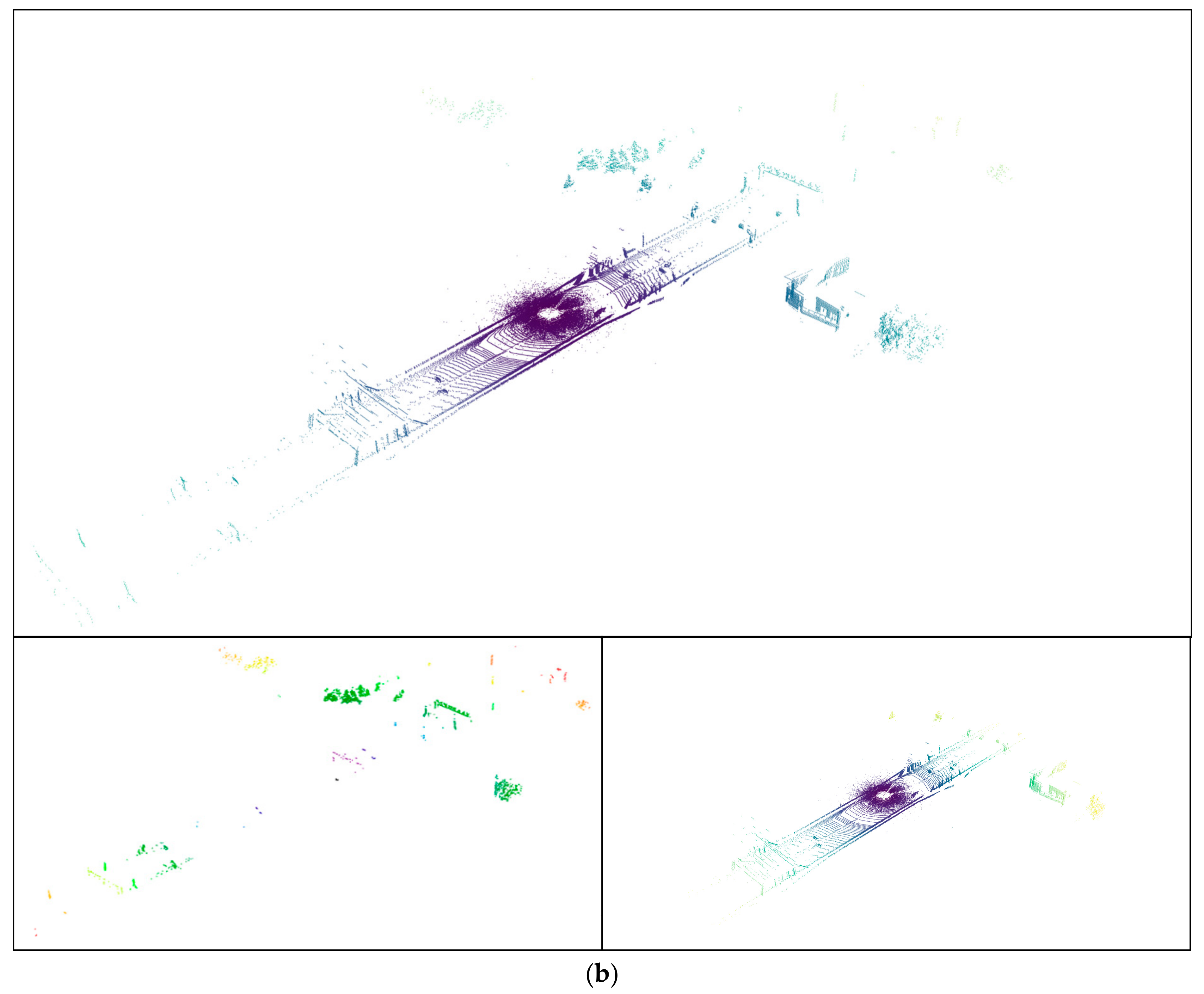
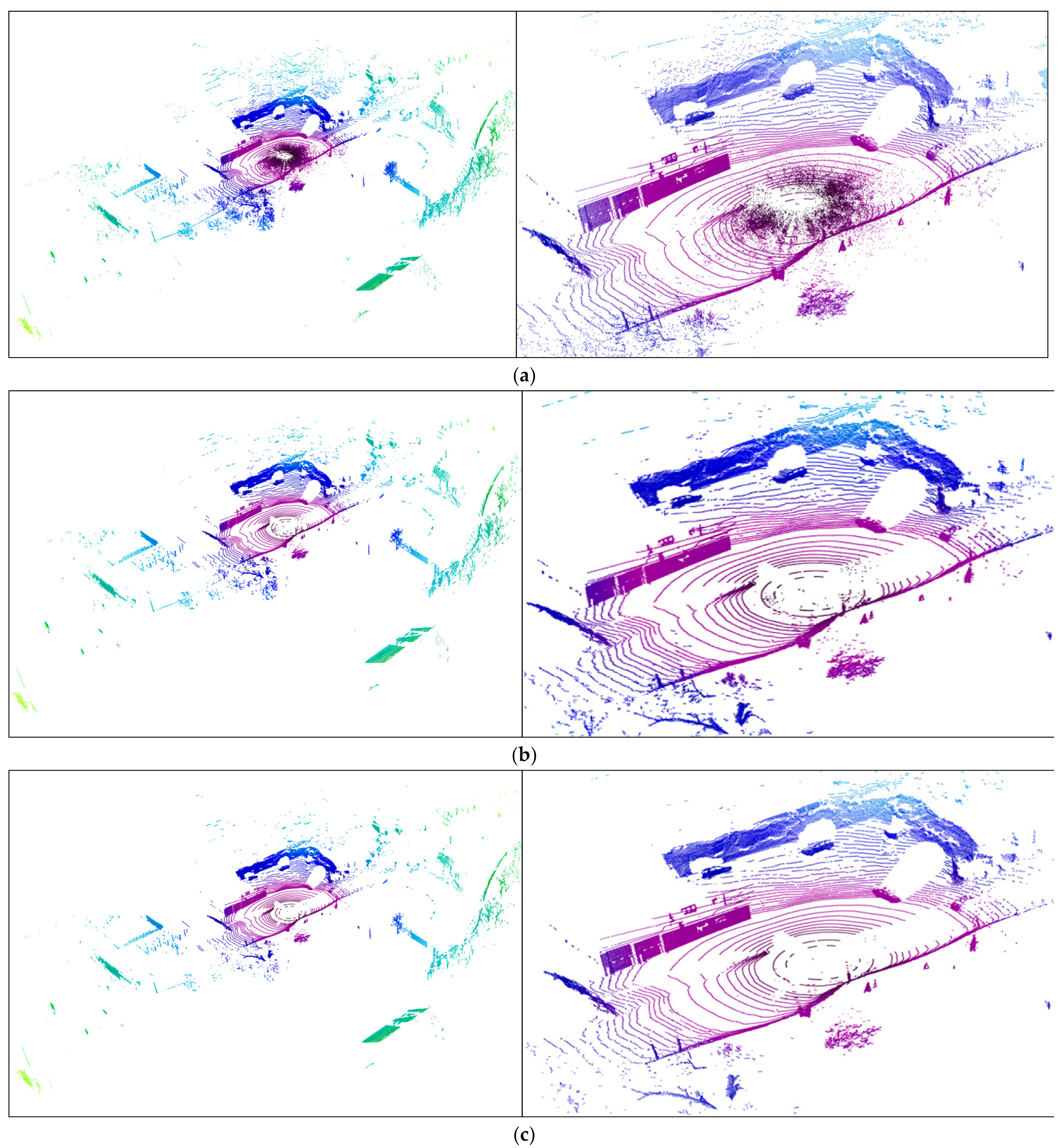
4.1. Qualitative Assessment

We compared the DSOR algorithm to the proposed DDIOR filter based on the results analyzed in Section 2. The parameters applied to the DSOR algorithm are summarized as follows: the number of neighbors was set to five, the global threshold constant was set to 0.01 and the range multiplicative factor was set to 0.05.

Figure 7 and Figure 8 show the visualization results of the original point cloud (the color map is spectral) after processing with the different filtering algorithms. They additionally show the point cloud filtering results of the 90th scan of sequences 23 and 26. Both figures are composed of three subgraphs, which from top to bottom are: the raw scan, the DSOR filtering results and the DDIOR filtering results. The left-hand side of each subgraph is the overall result and the right-hand side presents the details. DSOR, the best de-snowing algorithm available, retained environmental features while removing most of the snow accumulation. The proposed DDIOR filter, in contrast, removed more snow noise from the point cloud to yield a cleaner point cloud without losing environmental features.

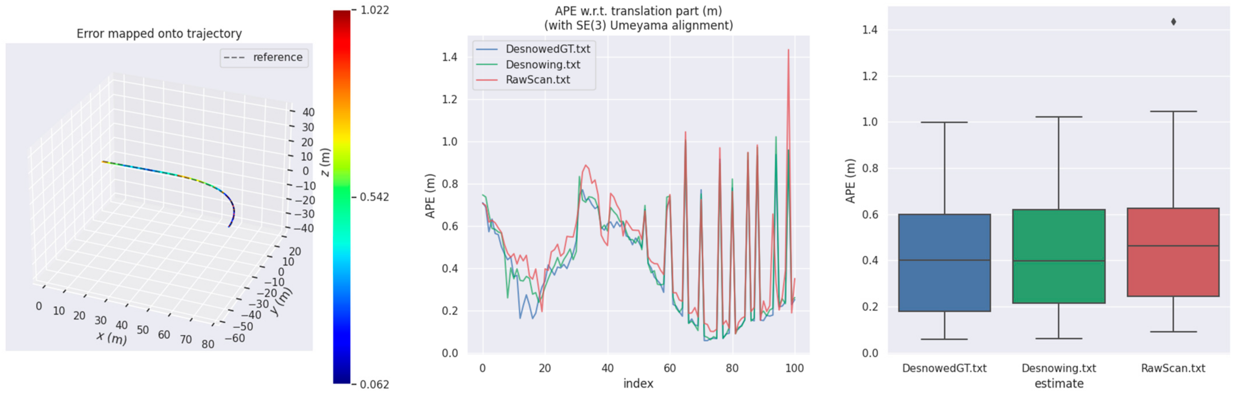
4.2. Quantitative Evaluation

We used classical indicators for the point cloud filtering assessments, i.e., precision and recall, to quantitatively evaluate the proposed method. The essence of point cloud filtering with snow noise is to filter out as many snow noise points as possible (recall) while fully preserving the detailed characteristics of the environment (precision). Aggressive filters can remove all snow noise points, but they inevitably filter out environmental details as well. Mild filters, in contrast, can accommodate more snow noise points; however, although the ambient features are retained, an excessive number of snow noise points impacts environmental perception. Therefore, efficiently balancing the precision and recall is an important metric for evaluating point cloud filtering algorithms. the precision and recall are defined as follows:

$$Precision=\frac{TP}{TP+FP},Recall=\frac{TP}{TP+FN}$$

(3)

where $TP$ stands for true positive, which refers to snow noise points filtered out from the point cloud; $FP$ stands for false positive, which refers to non-snow points filtered out from the point cloud; and $FN$ stands for false negative, which refers to snow noise points retained in the point cloud after filtering.

Table 12. A quantitative comparison between different filters.

Filters	Precision	Recall
DROR	71.51	91.89
DSOR	65.07	95.60
DDIOR	69.87	95.23

, which shows a comparison of DSOR and DDIOR in terms of precision and recall, clearly indicates that DDIOR achieved a higher de-snowing precision at the same recall.

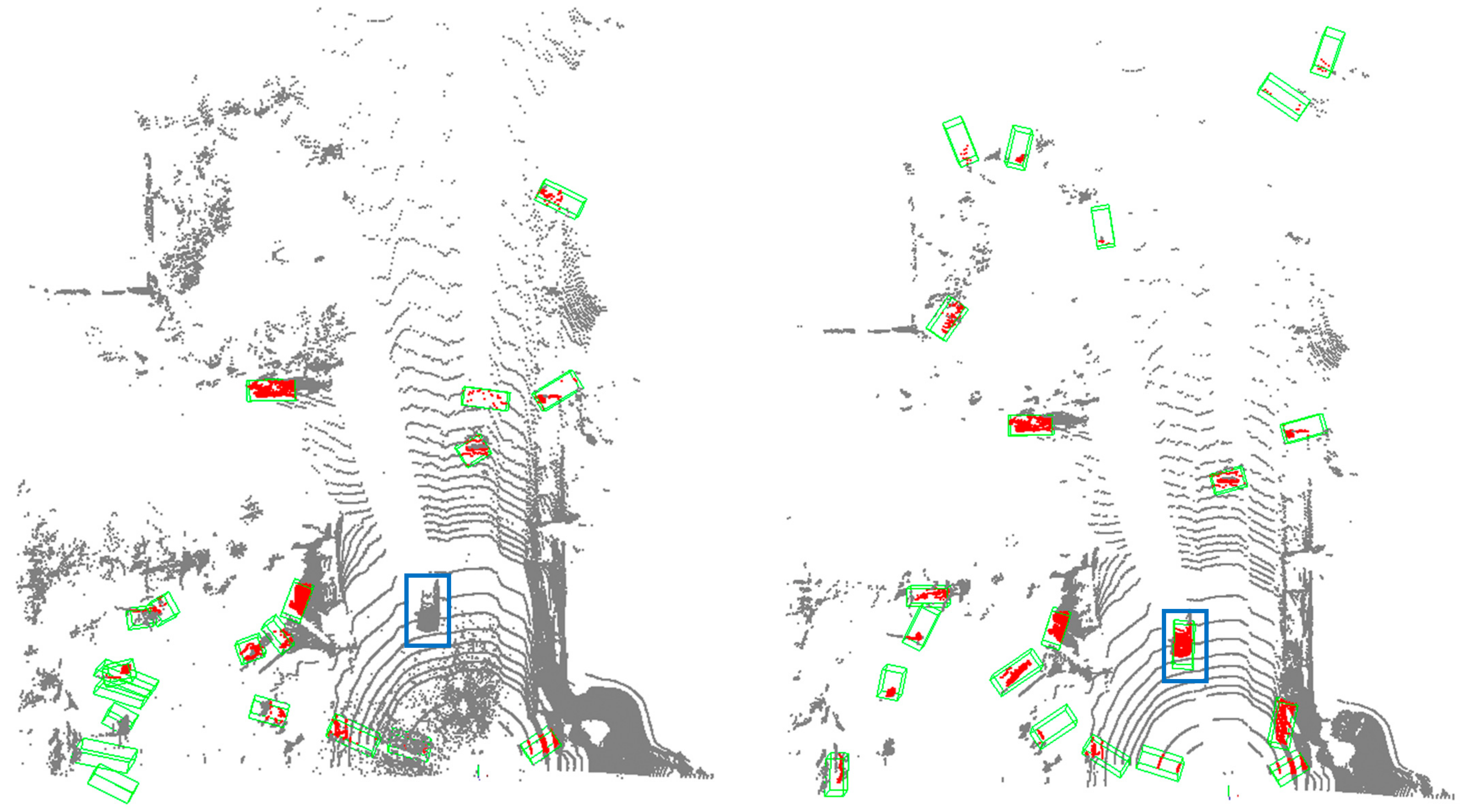
4.3. Other Applications

To fully reflect the practicability of our method, we first tested the mainstream environmental perception task of object detection and compared the perception effects on raw scans and de-snowing scans.

We selected Sparsely Embedded CONvolutional Detection (SECOND) [29] for object detection, which was initially proposed in 2018. The comparison data were the 90th scan of sequence 34. The results are shown in Figure 9. The left-hand figure shows the object detection results on the raw scan and the right-hand figure shows the object detection results on the de-snowing scan. The object detection result was clearly improved after snow removal and noise reduction. Although there was a certain false positive rate, the vehicle close to the LiDAR could not be detected on the raw scan, but the vehicle could be accurately detected on the de-snowing scan (shown in the blue rectangular box).

Subsequently, we choose the open-source SLAM algorithm called MULLS [30], which was published on ICRA2021, as the benchmark to compare the pose estimation results on raw scans and de-snowing scans. We used three kinds of input data for the experiments: raw scans, the scans that filtered out snow noise points using our DDIOR (abbreviated as Desnowing) and the scans that filtered out snow noise points according to semantic ground truth (abbreviated as DesnowedGT). For the evaluation of the SLAM algorithm, the quantitative evaluation index of absolute pose error (APE) was applied using Sim (3) Umeyama alignment in the calculation. We then used the evo tool [31] to evaluate the estimated pose results. Figure 10 shows the APE visualization results for the different inputs of sequence 24. It should be noted that each sequence in the WADS dataset only has about 100 scans. Due to the small amount of data, it had no significant impact on pose estimation, so we can only show the comparison results of the pose estimation of one sequence. Nevertheless, we can see that snow removal improves the overall pose estimation, which proves that our de-snowing algorithm is helpful for improving the environmental perception of autonomous vehicles.

5. Conclusions

The DDIOR filter proposed in this paper can improve the environmental perception capabilities of autonomous vehicles in severe weather conditions, especially snowy conditions. Specifically, on the basis of the annotated point-wise WADS dataset, the characteristics of LiDAR point cloud data collected under snowy conditions were systematically and accurately analyzed and a DDIOR filtering algorithm that includes data preprocessing, dynamic point cloud filtering and point cloud fusion was proposed. The core of the algorithm is the efficient and accurate removal of snow noise by setting dynamic filter coefficients that are based on the combination of the point-wise distance and intensity values within the point cloud data. The experimental results on WADS data show that DDIOR can achieve an effective balance between precision and recall. In summary, as a LiDAR point cloud de-noising technique, the proposed method can be used to enhance the environmental perception capabilities of autonomous vehicles in snowy conditions. In future research, we will continue to improve the ability of autonomous vehicles to perceive their environments efficiently and accurately under harsh weather conditions and in complex dynamic environments.

References

1. Yoneda, K.; Suganuma, N.; Yanase, R.; Aldibaja, M. Automated driving recognition technologies for adverse weather conditions. IATSS Res. 2019, 43, 253–262. [Google Scholar] [CrossRef]
2. Wang, H.; Yue, Z.; Xie, Q.; Xie, Q.; Zhao, Q.; Zheng, Y.; Meng, D. From Rain Generation to Rain Removal. In Proceedings of the IEEE/CVF Conference on Computer Vision and Pattern Recognition, Nashville, TN, USA, 20–25 June 2021; pp. 14791–14801. [Google Scholar]
3. Lin, S.L.; Wu, B.H. Application of Kalman Filter to Improve 3D LiDAR Signals of Autonomous Vehicles in Adverse Weather. Appl. Sci. 2021, 11, 3018. [Google Scholar] [CrossRef]
4. Zhang, Y.; Carballo, A.; Yang, H.; Takeda, K. Autonomous Driving in Adverse Weather Conditions: A Survey. arXiv 2021, arXiv:2112.089362112. [Google Scholar]
5. Kurup, A.; Bos, J. DSOR: A Scalable Statistical Filter for Removing Falling Snow from LiDAR Point Clouds in Severe Winter Weather. arXiv 2021, arXiv:2109.07078. [Google Scholar]
6. Park, J.I.; Park, J.; Kim, K.S. Fast and Accurate Desnowing Algorithm for LiDAR Point Clouds. IEEE Access 2020, 8, 160202–160212. [Google Scholar] [CrossRef]
7. Charron, N.; Phillips, S.; Waslander, S.L. De-noising of lidar point clouds corrupted by snowfall. In Proceedings of the 15th IEEE Conference on Computer and Robot Vision (CRV), Toronto, ON, Canada, 8–10 May 2018; pp. 254–261. [Google Scholar]
8. Heinzler, R.; Piewak, F.; Schindler, P.; Stork, W. Cnn-based lidar point cloud de-noising in adverse weather. IEEE Robot. Autom. Lett. 2020, 5, 2514–2521. [Google Scholar] [CrossRef] [Green Version]
9. Han, X.F.; Jin, J.S.; Wang, M.J.; Jiang, W.; Gao, L.; Xiao, L. review of algorithms for filtering the 3D point cloud. Signal Processing Image Commun. 2017, 57, 103–112. [Google Scholar] [CrossRef]
10. Narváez, E.A.L.; Narváez, N.E.L. Point cloud de-noising using robust principal component analysis. In Proceedings of the International Conference on Computer Graphics Theory and Applications, Setúbal, Portugal, 25–28 February 2006; pp. 51–58. [Google Scholar]
11. Jenke, P.; Wand, M.; Bokeloh, M.; Schilling, A.; Straßer, W. Bayesian point cloud reconstruction. In Computer Graphics Forum; Blackwell Publishing, Inc.: Oxford, UK; Boston, MA, USA, 2006; Volume 25, pp. 379–388. [Google Scholar]
12. Paris, S. A gentle introduction to bilateral filtering and its applications. In Proceedings of the ACM SIGGRAPH 2007 Courses, Los Angeles, CA, USA, 12–17 August 2001; Available online: https://dl.acm.org/doi/proceedings/10.1145/12815003-es (accessed on 20 February 2022).
13. Lipman, Y.; Cohen-Or, D.; Levin, D.; Tal-Ezer, H. Parameterization-free projection for geometry reconstruction. ACM Trans. Graph. (TOG) 2007, 26, 22. [Google Scholar] [CrossRef]
14. Huang, H.; Li, D.; Zhang, H.; Ascher, U.; Cohen-Or, D. Consolidation of unorganized point clouds for surface reconstruction. ACM Trans. Graph. (TOG) 2009, 28, 1–7. [Google Scholar] [CrossRef] [Green Version]
15. Rusu, R.B.; Cousins, S. 3D is here: Point cloud library (PCL). In Proceedings of the 2011 IEEE International Conference on Robotics and Automation, Shanghai, China, 9–13 May 2011. [Google Scholar]
16. Liu, S.; Chan, K.C.; Wang, C.C.L. Iterative consolidation of unorganized point clouds. IEEE Comput. Graph. Appl. 2011, 32, 70–83. [Google Scholar]
17. Balta, H.; Velagic, J.; Bosschaerts, W.; De Cubber, G.; Siciliano, B. Fast statistical outlier removal based method for large 3D point clouds of outdoor environments. IFAC-PapersOnLine 2018, 51, 348–353. [Google Scholar] [CrossRef]
18. Duan, Y.; Yang, C.; Chen, H.; Yan, W.; Li, H. Low-complexity point cloud de-noising for LiDAR by PCA-based dimension reduction. Opt. Commun. 2021, 482, 126567. [Google Scholar] [CrossRef]
19. Roriz, R.; Campos, A.; Pinto, S.; Gomes, T. “DIOR: A Hardware-Assisted Weather De-noising Solution for LiDAR Point Clouds. IEEE Sens. J. 2022, 22, 1621–1628. [Google Scholar] [CrossRef]
20. Piewak, F.; Pinggera, P.; Schafer, M.; Peter, D.; Schwarz, B.; Schneider, N.; Enzweiler, M.; Pfeiffer, D.; Zöllner, M. Boosting lidar-based semantic labeling by cross-modal training data generation. In Proceedings of the European Conference on Computer Vision (ECCV), Munich, Germany, 8–14 September 2018. [Google Scholar]
21. Geiger, A.; Lenz, P.; Stiller, C.; Urtasun, R. Vision meets robotics: The kitti dataset. Int. J. Robot. Res. 2013, 32, 1231–1237. [Google Scholar] [CrossRef] [Green Version]
22. Maddern, W.; Pascoe, G.; Linegar, C.; Newman, P. 1 year, 1000 km: The Oxford robotcar dataset. Int. J. Robot. Res. 2017, 36, 3–15. [Google Scholar] [CrossRef]
23. Huang, X.; Wang, P.; Cheng, X.; Zhou, D.; Geng, Q.; Yang, R. The apolloscape open dataset for autonomous driving and its application. IEEE Trans. Pattern Anal. Mach. Intell. 2019, 42, 2702–2719. [Google Scholar] [CrossRef] [PubMed] [Green Version]
24. Sun, P.; Kretzschmar, H.; Dotiwalla, X.; Chouard, A.; Patnaik, V.; Tsui, P.; Guo, J.; Zhou, Y.; Chai, Y.; Caine, B.; et al. Scalability in perception for autonomous driving: Waymo open dataset. In Proceedings of the IEEE/CVF Conference on Computer Vision and Pattern Recognition, Seattle, WA, USA, 13–19 June 2020; pp. 2446–2454. [Google Scholar]
25. Caesar, H.; Bankiti, V.; Lang, A.H.; Vora, S.; Liong, V.E.; Xu, Q.; Krishnan, A.; Pan, Y.; Baldan, G.; Beijbom, O. Nuscenes: A multimodal dataset for autonomous driving. In Proceedings of the IEEE/CVF Conference on Computer Vision and Pattern Recognition, Seattle, WA, USA, 13–19 June 2020; pp. 11621–11631. [Google Scholar]
26. Behley, J.; Garbade, M.; Milioto, A.; Quenzel, J.; Behnke, S.; Stachniss, C.; Gall, J. Semantickitti: A dataset for semantic scene understanding of lidar sequences. In Proceedings of the IEEE/CVF International Conference on Computer Vision, Seoul, Korea, 27 October–2 November 2019; pp. 9297–9307. [Google Scholar]
27. Bijelic, M.; Gruber, T.; Mannan, F.; Kraus, F.; Ritter, W.; Dietmayer, K.; Heide, F. Seeing through fog without seeing fog: Deep multimodal sensor fusion in unseen adverse weather. In Proceedings of the IEEE/CVF Conference on Computer Vision and Pattern Recognition, Seattle, WA, USA, 15 November 2020; pp. 11682–11692. [Google Scholar]
28. Pitropov, M.; Garcia, D.E.; Rebello, J.; Smart, M.; Wang, C.; Czarnecki, K.; Waslander, S. Canadian adverse driving conditions dataset. Int. J. Robot. Res. 2021, 40, 681–690. [Google Scholar] [CrossRef]
29. Yan, Y.; Mao, Y.; Li, B. SECOND: Sparsely Embedded Convolutional Detection. Sensors 2018, 18, 3337. [Google Scholar] [CrossRef] [PubMed] [Green Version]
30. Pan, Y.; Xiao, P.; He, Y.; Shao, Z.; Li, Z. MULLS: Versatile LiDAR SLAM via Multi-metric Linear Least Square. In Proceedings of the IEEE International Conference on Robotics and Automation (ICRA), Xi’an, China, 30 May–5 June 2021; pp. 11633–11640. [Google Scholar] [CrossRef]
31. Grupp, M. Evo: Python PackAge for the Evaluation of Odometry and Slam. Available online: https://github.com/MichaelGrupp/evo (accessed on 10 March 2022).
Figure 1. The visualization results of the WADS dataset. The left-hand image is the raw scan (visualizing with distance values and the color map is viridis) and the right-hand image is the point cloud with semantic annotation (each black point indicates a snow noise point).
Remotesensing 14 01468 g001
Figure 2. The corresponding relationship between r , x , y , z and i under snowy conditions: (a) sequence 11; (b) sequence 12; (c) sequence 13.
Remotesensing 14 01468 g002aRemotesensing 14 01468 g002b
Figure 3. The corresponding relationship between r , x , y , z and i under sunny conditions: (a) sequence 01; (b) sequence 02; (c) sequence 03.
Remotesensing 14 01468 g003aRemotesensing 14 01468 g003b
Figure 4. Statistics regarding the data proportion of snow noise points and non-snow points.
Remotesensing 14 01468 g004
Figure 5. A schematic diagram of the data preprocessing (the data presented is the 80th scan of sequence 22). (a) is the schematic diagram of the data distribution in which the left-hand figure is the original data and the green dotted line is the threshold line. The next step of the filtering processing was carried out on the area data in the lower left-hand corner of the intersection of the threshold line and the data in the other areas were retained. The figure on the right shows the overall distribution of the data to be filtered. (b) is the visualization of the data preprocessing: the top image is the raw scan, the lower left-hand image is the retained data and the lower right-hand image is the subsequent dynamic filtering data.
Remotesensing 14 01468 g005aRemotesensing 14 01468 g005b
Figure 6. (a) the visualization result of the raw scan, and (b) shows that if only the intensity value is used as the filtering parameter.
Remotesensing 14 01468 g006
Figure 7. A qualitative comparison of the state-of-the-art DSOR and our DDIOR on the 90th scan of sequence 23: (a) The raw scan; (b) DSOR; (c) DDIOR. The left-hand images show the visualization results of the overall filtering effect and the right-hand images show the visualization results of the filtering details.
Remotesensing 14 01468 g007
Figure 8. A qualitative comparison of the state-of-the-art DSOR and our DDIOR on the 90th scan of sequence 26: (a) The raw scan; (b) DSOR; (c) DDIOR. The left-hand images show the visualization results of the overall filtering effect and the right-hand images show the visualization results of the filtering details.
Remotesensing 14 01468 g008
Figure 9. A qualitative comparison of the raw scan and the de-snowing scan in terms of object detection.
Remotesensing 14 01468 g009
Figure 10. Comparisons of the APE used as the translation component of different inputs based on the MULLS.
Remotesensing 14 01468 g010