Sea Surface Skin Temperature Retrieval from FY-3C/VIRR

Abstract

The visible and infrared scanning radiometer (VIRR) onboard the Fengyun-3C (FY-3C) meteorological satellite has 11 μm and 12 μm channels, which are capable of sea surface temperature (SST) observations. This study is based on atmospheric radiative transfer modeling (RTM) by applying Bayesian cloud detection theory and optimal estimation (OE) to obtain sea surface skin temperature (${\mathrm{SST}}_{\mathrm{skin}}$) from VIRR in the Northwest Pacific. The inter-calibration of FY-3C/VIRR 11 μm and 12 μm brightness temperature (BT) is carried out using the Moderate Resolution Imaging Spectroradiometer (MODIS) as the reference sensor. Bayesian cloud detection and OE SST retrieval with the calibration BT data is performed to obtain ${\mathrm{SST}}_{\mathrm{skin}}$. The ${\mathrm{SST}}_{\mathrm{skin}}$ retrievals are compared with the buoy SST with a temporal window of 1 h and a spatial window of 0.01°. The bias is −0.12 °C, and the standard deviation is 0.52 °C. Comparisons of the retrieved ${\mathrm{SST}}_{\mathrm{skin}}$ with the AVHRR (Advanced Very High Resolution Radiometer) ${\mathrm{SST}}_{\mathrm{skin}}$ from European Space Agency Sea Surface Temperature Climate Change Initiative (ESA SST CCI) project show the bias of 0.08 °C and the standard deviation of 0.55 °C. The results indicate that the VIRR ${\mathrm{SST}}_{\mathrm{skin}}$ are consistent with AVHRR ${\mathrm{SST}}_{\mathrm{skin}}$ and buoy SST.

1. Introduction

Sea Surface Temperature (SST) is one of the critical indicators that characterizes changes in the marine environment and climate. Many ocean dynamic processes are related to SST; thus, SST has been widely used in ocean dynamics research and air–sea interactions, such as studying El Niño and La Niña phenomena and the analysis of Kuroshio and Gulf Streams [1,2]. SST is an important indicator of climate change and has been applied to climate change monitoring [2]. SST has also been used for weather forecast [3], marine fishery monitoring [4], etc. Most satellite SST data are required for an accuracy of about 0.5 °C when applied at high spatial resolution (0.5~10 km) [5]. The SST data used to study climate change requires higher accuracy of about 0.1 °C [6].

The operational infrared SST observation has a history of four decades. The Advanced Very High Resolution Radiometer (AVHRR) is onboard the National Oceanic and Atmospheric Administration (NOAA, Washington, DC, USA) and MetOp (Meteorological Operational) series meteorological satellites, and the Nonlinear SST (NLSST) algorithms have been used to retrieve SST [7]. The result of comparing MetOp-A/AVHRR operational SST with buoy SST shows that the bias during the day is 0.05 °C and the standard deviation is 0.61 °C; the bias of night data is −0.03 °C, and the standard deviation is 0.48 °C [8]. The Moderate Resolution Imaging Spectroradiometer (MODIS) onboard Terra and Aqua satellites is an essential sensor for observing SST. Its operational SST algorithm is also NLSST [9]. The result of comparing MODIS SST with buoy SST from 2002 to 2011 shows that the bias of the two is −0.13 °C, and the standard deviation is 0.58 °C [10]. The Visible Infrared Imaging Radiometer Suite (VIIRS) is a mid-resolution visible infrared imager, it uses the NLSST algorithm for SST retrieval during the day and the Multi-Channel SST retrieval Algorithm (MCSST) at night [11]. According to the evaluation of the VIIRS SST with the buoy SST on the NOAA SQUAM (SST Quality Monitor) [12], the 2016 Suomi-NPP/VIIRS SST has a bias of 0.04 °C and a standard deviation of 0.37 °C in the daytime and a bias of 0.07 °C and a standard deviation of 0.29 °C at night [13]. The Along Track Scanning Radiometers (ATSRs) are multi-channel sensors; the fourth-generation ATSR series onboard the Sentinel-3A and Sentinel-3B satellites is Sea and Land Surface Temperature Radiometer (SLSTR). The SLSTR SST is retrieved by a fitting algorithm using the atmospheric radiative transfer modeling [14]. Compared with M-AERIs SST from 2017 to 2018, Sentinel-3A SLSTR SST has a bias of −0.098 °C and a robust standard deviation (RSD) of 0.296 °C [15].

The Fengyun-3 (FY-3) meteorological satellites are Chinese second-generation polar-orbiting meteorological satellites. The orbits of polar-orbiting satellites are sun-synchronous orbits, which means they theoretically pass the equator at the same local time every day [16]. The FY-3A and FY-3B satellites are experimental satellites; they were launched in 2008 and 2010, respectively. FY-3C, launched on 23 September 2013, is the first operational satellite of the FY-3 series. It passes through the equator at 10:00~10:20 a.m. The VIRR is mounted on the FY-3C satellite. It has 10 spectral channels, and three channels can be used for SST retrieval. They are channel 3 in the range of 3.55–3.93 μm, channel 4 in the range of 10.3–11.3 μm, and channel 5 in the range of 11.5–12.5 μm [17]. The operational SST retrieval algorithm of FY-3C/VIRR is the MCSST algorithm. The MCSST algorithm coefficients are obtained from the regression analysis of the buoy SST and VIRR infrared channel brightness temperature (BT). The comparison of operational VIRR SST and buoy SST from May 2014 to June 2014 show that during the day, the bias is −0.26 °C and the standard deviation is 0.54 °C; at night, the bias is 0.06 °C and the standard deviation is 0.56 °C [17]. Compared with the Optimum Interpolation Sea Surface Temperature (OISST), the bias during the day is −0.33 °C, the standard deviation is 0.94 °C; the bias at night is −0.10 °C, and the standard deviation is 0.76 °C [17]. Comparing the third edition operational SST with the buoy, the bias during the day and night are 0.17 °C and 0.07 °C, respectively, and the standard deviation is less than 0.54 °C [18]. The results of comparison between OISST and the VIRR SST with the highest quality from January to May 2017 show that the bias of the SST during the day is −0.1 °C and the standard deviation is 0.8 °C; the bias at night is 0.01 °C and the standard deviation is 0.78 °C [18]. The validation results of FY-3C/VIRR SST with OISST from January 2015 to December 2019 show that the SST with the highest quality level has a bias of −0.18 °C and a root mean square error of 0.85 °C during the day and a bias of −0.06 °C and a root mean square error of 0.8 °C at night. The root mean square error is 0.85 °C and 0.8 °C, respectively [19]. Monthly NLSST regression coefficients are used to reprocess FY-3C/VIRR data. Comparing the highest quality SST data of the Western Pacific in March, May, August, and November 2016 with the buoy, the bias of matchups during the day is 0.02 °C and the standard deviation is 0.62 °C; at night, the bias of the matchups is 0.14 °C and the standard deviation is 0.58 °C [20].

The sea surface in most cases is warmer than the atmosphere in contact with it, causing heat to flow from the ocean to the atmosphere [21]. Because the air–sea density difference and the near-surface viscous layer on the seawater side of the air–sea interface suppresses turbulent heat transfer, there is a vertical temperature gradient in the water just below the interface, resulting in a decrease in temperature near the air–sea interface [22]. The FY-3C/VIRR operational SST is retrieved using coefficients fitted by buoy SST and satellite observation BT [18]. The depth of obtained SST is close to the buoy, which represents the bulk temperature [18], while the infrared sensors observe the skin SST with the depth of 10 μm [23]. Merchant proposed an optimal estimation (OE) SST retrieval method in 2008. The OE SST algorithm obtains sea surface skin temperature (${\mathrm{SST}}_{\mathrm{skin}}$) with radiative transfer modelling [24]. This study intends to obtain the FY-3C/VIRR sea surface skin temperature (${\mathrm{SST}}_{\mathrm{skin}}$) by atmospheric radiative transfer modelling. In Section 2, data and methods used in this study are introduced. The methods include the inter-calibration, Bayesian cloud detection, and OE SST retrieval algorithm. In Section 3, the analysis of results is described. Section 4 and Section 5 are Discussion and Conclusions, respectively.

2. Materials and Methods

2.1. Data Collections

2.1.1. FY-3C/VIRR L1B Data

VIRR has spectral channels, with a spectral coverage range of 0.43 µm to 12.5 µm. The spectral specifications are shown in Table 1 [25]. Its nadir resolution is 1.1 km, the scan width is ±55.4°, and the swath width is 2800 km. The VIRR L1B data is 5-min swath data, and the data format is HDF5 [25]. This study applies the BT of 11 µm and 12 µm to retrieve SST. The geographic information includes longitude, latitude, satellite zenith angle, solar zenith angle, etc. Longitude and latitude are used for geographic correction in subsequent matching and validation, satellite zenith angle is used for matching with MODIS, and solar zenith angle is used for judging day or night. The spatial range is 2°S~46°N, 121°E~160°E. We selected March, May, August, and November to represent seasonal characteristics in this region. The VIRR L1B data is distributed by the National Satellite Meteorological Center (NSMC, China); the data version we used is V1.0.0.

Table 1. FY-3C/VIRR spectrum specifications [25].

Channel	Band Range (μm)	Noise Equivalent Reflectivity ρ(%) Noise Equivalent Temperature Difference (300 K)	Dynamic Range
1	0.58–0.68	0.10%	0–100%
2	0.84–0.89	0.10%	0–100%
3	3.55–3.93	0.3 K	180–350 K
4	10.3–11.3	0.2 K	180–330 K
5	11.5–12.5	0.2 K	180–330 K
6	1.55–1.64	0.15%	0–90%
7	0.43–0.48	0.05%	0–50%
8	0.48–0.53	0.05%	0–50%
9	0.53–0.58	0.05%	0–50%
10	1.325–1.395	0.19%	0–90%

2.1.2. TERRA/MODIS L1B Data

Terra is also a polar-orbiting satellite. The descending node of Terra is at 10:30 am, which is close to FY-3C. Therefore, MODIS onboard Terra is used in this study for the purpose of inter-calibration. The swath width of MODIS is 2330 km. Among 36 channels of MODIS, channels 20, 22, 23, 31, and 32 are used for SST retrieval [26]. The nadir resolution of channel 31 and channel 32 is 1 km [26]. The data format is HDF4. In addition to BT information, MODIS L1B data also includes latitude and longitude, satellite zenith angle, etc., which are used for geographic correction and matching with VIRR data. The MODIS L1B data is distributed by Level-1 and Atmosphere Archive and Distribution System Distributed Active Archive Center (LAADS DAAC), and the MODIS L1B data version is V6.2.2.

2.1.3. Metop-A/AVHRR SST_skin Data

The AVHRR is mounted on Metop-A, the local time of the descending node is 9:30 am, which is close to the FY-3C satellite. Merchant et al. reprocessed the AVHRR data and used the optimal estimation algorithm for SST retrieval [27]. Next, a climate data record (CDR) of global SST had been developed. The SST is skin SST in the depth of 10 μm [27]. This study uses AVHRR L2P ${\mathrm{SST}}_{\mathrm{skin}}$ data from the CDR to validate the retrieval results. Its nadir resolution is 4 km. AVHRR ${\mathrm{SST}}_{\mathrm{skin}}$ contains quality level information. The quality level of SST was divided according to land and ice information, SST value range, clear sky probability, zenith angle information, etc. for users to choose [27]. Pixels that pass all checks have the highest quality with a quality level of 5. The AVHRR ${\mathrm{SST}}_{\mathrm{skin}}$ data are from European Space Agency Sea Surface Temperature Climate Change Initiative (ESA SST CCI) project and the version is V2.1.

2.1.4. Buoy Data

The buoy data are from iQuam (In situ SST Quality Monitor) SST data. The iQuam SST data include ship data, drifting buoy data, tropical moored buoy data, coastal moored buoy data, Argo Float data, high resolution drifter data, IMOS (Integrated Marine Observing System, Australia) data, and CRW (coral reef buoy) data. The iQuam data also contain quality level information. The quality level of iQuam data was divided based on duplicate removal, plausibility/geolocation check, platform track check, SST spike check, ID check, reference check, and cross-platform check [28]. The data with quality level of 5 have the highest quality level. This study selects only the highest quality drifting buoy data, tropical moored buoy data, and high resolution drifter data for validation [28]. Buoys, moored buoys, as well as high resolution drifters measure water temperature in the depth of 10⁻²~10 m, the temperature is bulk temperature [23]. The data were downloaded from the National Environmental Satellite, Data, and Information Service Satellite Applications and Research (NOAA NESDIS STAR) center; the iQuam data version of this study used is V2.1.

2.1.5. ERA-Interim Data

ERA-Interim numerical weather prediction (NWP) data include atmospheric parameters and surface parameters. Atmospheric parameters include temperature, specific humidity, ozone mass mixing ratio, and specific cloud liquid water content. Surface parameters mainly include sea surface temperature, ${\mathrm{SST}}_{\mathrm{skin}}$, surface pressure, total column water vapor (TCWV), total cloud cover, 10 m U wind component, 10 m V wind component, 2 m temperature, and 2 m dewpoint temperature. In addition, geolocation information, such as latitude and longitude, are also included here. The spatial resolution of NWP data is 75 km, with data at 0 h, 6 h, 12 h, and 18 h every day [29]. The NWP data was downloaded from the European Centre for Medium-Range Weather Forecasts (ECMWF).

2.2. Inter-Calibration with MODIS L1B BT Data

FY-3C and Terra satellites cross the equator in close time. The center wavelengths of MODIS channels 31 and 32 and those of VIRR channels 4 and 5 are close. The channels 31 and 32 of MODIS have excellent stability and experience tiny changes every year with less than 0.5% in long time series responses [30], which is often used to validate the accuracy of other sensors or as a reference sensor for the purpose of inter-calibration of other sensors [31]. In addition, the retrieval of OE SST essentially uses the difference between the satellite observed BT and the simulated BT to estimate the difference between the background SST and the SST combining with the sensitivity data, and then obtains the SST based on the background SST [24]. The SST accuracy depends on the difference between the satellite observation BT and the simulated BT. Therefore, the accuracy of the satellite observation BT is crucial for the retrieval of the OE SST. Using MODIS as the reference sensor, the BT data of VIRR and MODIS are inter-calibrated. The specific process of inter-calibration is shown in Figure 1. Firstly, the VIRR and MODIS L1B data, VIRR_BT and MODIS_BT, are projected into a 0.01° × 0.01° grid. For example, the BTs of both 11 μm and 12 μm channels after projection in the daytime of 28 March 2016 are shown in Figure 2. To generate the matchups, the temporal window is set to 20 min. The matchups with the local standard deviation (LSD) of the BT less than 0.1 K and the satellite zenith angle less than 5° are selected in order to reduce the influence of different atmospheric path lengths and improve the homogeneity.

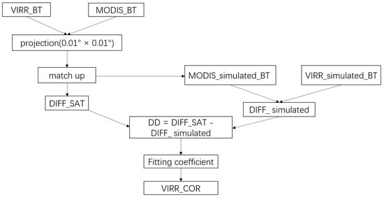
Figure 1. Inter-calibration process of VIRR_BT and MODIS_BT.

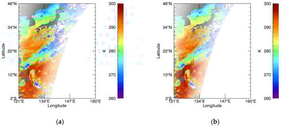
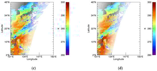
Figure 2. VIRR_BT and MODIS_BT after projection in the daytime of 28 March 2016: (a) VIRR 11 μm channel; (b) MODIS 11 μm channel; (c) VIRR 12 μm channel; (d) MODIS 12 μm channel.

The difference between VIRR_BT and MODIS_BT is named DIFF_SAT. The difference of the simulated BT (the spectral difference) of the two is named DIFF_simulated. Due to the difference of the sensor spectral response functions, it is necessary to use the DIFF_SAT minus DIFF_simulated to obtain the actual difference named DD (Double Difference). The BTs are simulated by the MODerate resolution atmospheric TRANsmission (MODTRAN). The difference between the simulated BT of the two is shown in Table 2. Figure 3 shows the relationship between the two simulated BTs. There are 411,100 matchups in the daytime and 397,902 matchups in the nighttime. From Table 2 and Figure 3, we can see that the VIRR simulated BTs of the 11 μm and 12 μm channels are lower than MODIS. The spectral difference of the 12 μm channel is more significant than that of the 11 μm channel. The spectral difference between the two channels has no apparent relationship with the time (daytime or nighttime). Table 3 shows the statistical results of DD. Figure 4 shows the relationship between the MODIS_BT plus the spectral difference and the VIRR_BT. The value of MODIS_BT plus the spectral difference is the value of MODIS_BT that removed the spectral difference with VIRR. From Table 3 and Figure 4, we can see that in the daytime the VIRR_BT of 11 μm and 12 μm channels is lower than that of MODIS, and the 12 μm channel is more obvious in areas with lower BT. In the nighttime, the VIRR_BT of the 11 μm channel is close to MODIS, the VIRR_BT of the 12 μm channel is higher than that of MODIS, and the 12 μm channel is more obvious in the area with higher BT. The DD between VIRR_BT and MODIS_BT in the daytime is larger than that in the nighttime.

Table 2. VIRR and MODIS simulated BT difference (D means daytime, N means nighttime, R means correlation coefficient).

	11 μm			12 μm
	Mean (K)	Std Dev (K)	R	Mean (K)	Std Dev (K)	R	Number
D	−0.31	0.10	0.9999	−0.97	0.15	0.9999	411,100
N	−0.33	0.10	0.9999	−0.86	0.21	0.9997	397,902

Figure 3. The relationship between VIRR and MODIS simulated BT: (a) 11 μm in the daytime; (b) 12 μm in the daytime; (c) 11 μm in the nighttime; (d) 12 μm in the nighttime.

Table 3. The Double Difference between VIRR_BT and MODIS_BT (D means daytime, N means nighttime, R means correlation coefficient).

	11 μm			12 μm
	Mean (K)	Std Dev (K)	R	Mean (K)	Std Dev (K)	R	Number
D	−0.93	0.27	0.9989	−0.53	0.31	0.9985	411,100
N	0.13	0.28	0.9991	0.44	0.32	0.9989	397,902

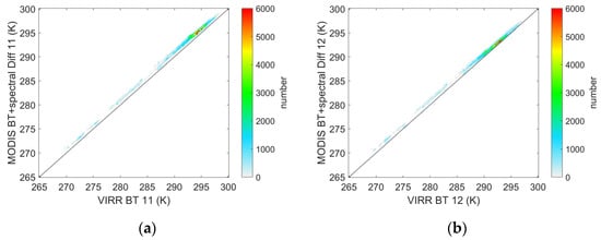
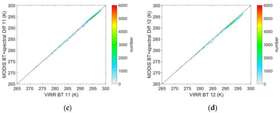
Figure 4. The relationship between MODIS_BT plus the spectral difference and VIRR_BT: (a) 11 μm in the daytime; (b) 12 μm in the daytime; (c) 11 μm in the nighttime; (d) 12 μm in the nighttime.

The MODIS_BTs with the spectral difference are used to calibrate the VIRR_BTs using Equations (1) and (2). The fitting coefficients of scale and offset are obtained, respectively, for 11 μm channel in the daytime, 12 μm channel in the daytime, 11 μm channel in the nighttime, and 12 μm channel in the nighttime.

VIRR_BT′ = scale × VIRR_BT + offset

(1)

VIRR_BT′ = MODIS_BT + Diff_simulated

(2)

The fitting coefficients are used to correct VIRR_BT to obtain the corrected BT named VIRR_COR. The VIRR L1B BTs before and after the correction and the difference between the two are shown in Figure 5 where the gray areas are the pixels exceeding the study area, land, and obviously cloud (pixels with the BT of 11 μm channel less than 260 K). Figure 5a–f show the images at 1:50 UTC on 28 March 2016 in the daytime, and Figure 5g–l show the images at 12:40 UTC on 11 May 2016 in the nighttime. Figure 5a–c,g–i show the 11 μm channel images, and others show the 12 μm channel images. After calibration, in the daytime, the BT of 11 μm and 12 μm channels is higher than that before calibration. The BT of the 12 μm channel is higher in the lower BT region. In the nighttime, the BT of 11 μm channel is close to that before calibration. The corrected BT of the 12 μm channel is lower in the area with higher BT than before correction, indicating that the accuracy of VIRR_COR after correction is higher than before.

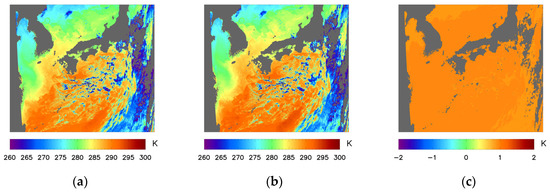
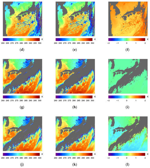
Figure 5. VIRR LI BT before and after calibration and the difference: (a) VIRR_BT 11 μm (daytime); (b) VIRR_COR 11 μm (daytime); (c) difference 11 μm (daytime); (d) VIRR_BT 12 μm (daytime); (e) VIRR_COR 12 μm (daytime); (f) difference 12 μm (daytime); (g) VIRR_BT 11 μm (nighttime); (h) VIRR_COR 11 μm (nighttime); (i) difference 11 μm (nighttime); (j) VIRR_BT 12 μm (nighttime); (k) VIRR_COR 12 μm (nighttime); (l) difference 12 μm (nighttime) (The gray areas are the pixels exceeding the study area, land, and obviously cloud (pixels with the BT of 11 μm channel less than 260 K)).

The difference between the VIRR_COR and MODIS_BT should be close to the spectral difference. The statistical results are shown in Table 4. The result of DD after correction is shown in Table 5. It shows that the DD of the two is close to 0 K, the standard deviation is within 0.3 K, the correlation coefficients are close to 1. The relationship between MODIS_BT plus the spectral difference and the VIRR_COR is shown in Figure 6. It can be seen that, in general, the 11 μm channel and 12 μm channel BT in the daytime and nighttime after calibration are in good agreement with the MODIS_BT plus the spectral difference. Improvements have been made to the low observed BT of 11 μm channel and 12 μm channel in the daytime and the high observed BT of 12 μm channel in the nighttime.

Table 4. Difference of VIRR_COR and MODIS_BT (D means daytime, N means nighttime, R means correlation coefficient).

	11 μm			12 μm
	Mean (K)	Std Dev (K)	R	Mean (K)	Std Dev (K)	R	Number
D	−0.31	0.25	0.9990	−0.97	0.32	0.9985	411,100
N	−0.34	0.25	0.9993	−0.86	0.34	0.9987	397,902

Table 5. DD between VIRR_COR and MODIS_BT (D means daytime, N means nighttime, R means correlation coefficient).

	11 μm			12 μm
	Mean (K)	Std Dev (K)	R	Mean (K)	Std Dev (K)	R	Number
D	0.00	0.27	0.9989	0.00	0.29	0.9991	411,100
N	−0.01	0.28	0.9985	0.01	0.28	0.9989	397,902

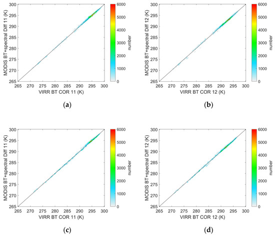
Figure 6. The relationship between MODIS_BT plus the spectral difference and VIRR_COR: (a) 11 μm in the daytime; (b) 12 μm in the daytime; (c) 11 μm in the nighttime; (d) 12 μm in the nighttime.

2.3. Cloud Detection

Bayesian cloud detection theory can provide the probability that the pixel is clear sky, so as to meet the needs of different users; therefore, this study adopts the Bayesian cloud detection method for cloud detection [32]. Bayesian cloud detection was proposed by Merchant, the formula is shown in Equation (3) [32].

$$\mathrm{P}\left({\mathrm{c}|\mathrm{y}}^{\mathrm{o}},{\mathrm{x}}^{\mathrm{b}}\right)={\left[1+\frac{\mathrm{P}\left(\overline{\mathrm{c}}\right)\mathrm{P}\left({\mathrm{y}}^{\mathrm{o}}{|\mathrm{x}}^{\mathrm{b}},\overline{\mathrm{c}}\right)}{\mathrm{P}\left(\mathrm{c}\right)\mathrm{P}\left({\mathrm{y}}^{\mathrm{o}}{|\mathrm{x}}^{\mathrm{b}},\mathrm{c}\right)}\right]}^{-1}$$

(3)

where $\mathrm{P}\left({\mathrm{c}|\mathrm{y}}^{\mathrm{o}},{\mathrm{x}}^{\mathrm{b}}\right)$ is the probability of a clear sky pixel, $\mathrm{P}\left(\mathrm{c}\right)$ is the prior cloud probability, $\mathrm{P}\left(\overline{\mathrm{c}}\right)$ is the prior clear probability, $\mathrm{P}\left({\mathrm{y}}^{\mathrm{o}}{|\mathrm{x}}^{\mathrm{b}},\mathrm{c}\right)$ is the probability density function (PDF) of the observation when the background field value is known under cloud conditions, $\mathrm{P}\left({\mathrm{y}}^{\mathrm{o}}{|\mathrm{x}}^{\mathrm{b}},\overline{\mathrm{c}}\right)$ is the PDF of the observation when the background field value is known under clear sky conditions. Both $\mathrm{P}\left({\mathrm{y}}^{\mathrm{o}}{|\mathrm{x}}^{\mathrm{b}},\mathrm{c}\right)$ and $\mathrm{P}\left({\mathrm{y}}^{\mathrm{o}}{|\mathrm{x}}^{\mathrm{b}},\overline{\mathrm{c}}\right)$ can be expressed as the product of the spectral part and the texture part, as shown in Equations (4) and (5) [32].

$$\mathrm{P}\left({\mathrm{y}}^{\mathrm{o}}{|\mathrm{x}}^{\mathrm{b}},\mathrm{c}\right)=\mathrm{P}\left({\mathrm{y}}_{\mathrm{s}}^{\mathrm{o}}{|\mathrm{x}}^{\mathrm{b}},\mathrm{c}\right)\times \mathrm{P}\left({\mathrm{y}}_{\mathrm{t}}^{\mathrm{o}}{|\mathrm{x}}^{\mathrm{b}},\mathrm{c}\right)$$

(4)

$$\mathrm{P}\left({\mathrm{y}}^{\mathrm{o}}{|\mathrm{x}}^{\mathrm{b}},\overline{\mathrm{c}}\right)=\mathrm{P}\left({\mathrm{y}}_{\mathrm{s}}^{\mathrm{o}}{|\mathrm{x}}^{\mathrm{b}},\overline{\mathrm{c}}\right)\times \mathrm{P}\left({\mathrm{y}}_{\mathrm{t}}^{\mathrm{o}}{|\mathrm{x}}^{\mathrm{b}},\overline{\mathrm{c}}\right)$$

(5)

where $\mathrm{P}\left({\mathrm{y}}_{\mathrm{s}}^{\mathrm{o}}{|\mathrm{x}}^{\mathrm{b}},\mathrm{c}\right)$ is the PDF of the spectral part under cloud conditions, $\mathrm{P}\left({\mathrm{y}}_{\mathrm{t}}^{\mathrm{o}}{|\mathrm{x}}^{\mathrm{b}},\mathrm{c}\right)$ is the PDF of texture part under cloud conditions, $\mathrm{P}\left({\mathrm{y}}_{\mathrm{s}}^{\mathrm{o}}{|\mathrm{x}}^{\mathrm{b}},\overline{\mathrm{c}}\right)$ is the PDF of the spectral part under clear sky conditions, $\mathrm{P}\left({\mathrm{y}}_{\mathrm{t}}^{\mathrm{o}}{|\mathrm{x}}^{\mathrm{b}},\overline{\mathrm{c}}\right)$ is the PDF of texture part under clear sky conditions.

Firstly, simulated BTs are obtained by MODTRAN with inputs of the Era-Interim NWP background field data, satellite zenith angle data, VIRR 11 μm and 12 μm spectral response curves and other information. Simulated BT is obtained through atmospheric radiative transfer modelling. The simulated BT of two channels at 1:50 UTC on 28 March 2016 is shown in Figure 7. The gray areas are the pixels exceeding the study area, land, and obviously cloud.

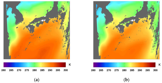
Figure 7. Simulated BT of two channels at 1:50 UTC on 28 March 2016: (a) 11 μm channel; (b) 12 μm channel (The gray areas are the pixels exceeding the study area, land, and obviously cloud (pixels with the BT of 11 μm channel less than 260 K)).

Based on the simulated BT, the corrected satellite observation BT, the satellite zenith angle, the background field total cloud cover, SST, TCWV, and other data, pixel-by-pixel calculations are performed to obtain the $\mathrm{P}\left({\mathrm{c}|\mathrm{y}}^{\mathrm{o}},{\mathrm{x}}^{\mathrm{b}}\right)$. In this process, it is necessary to calculate the $\mathrm{P}\left({\mathrm{y}}_{\mathrm{s}}^{\mathrm{o}}{|\mathrm{x}}^{\mathrm{b}},\mathrm{c}\right)$, $\mathrm{P}\left({\mathrm{y}}_{\mathrm{t}}^{\mathrm{o}}{|\mathrm{x}}^{\mathrm{b}},\mathrm{c}\right)$, $\mathrm{P}\left({\mathrm{y}}_{\mathrm{s}}^{\mathrm{o}}{|\mathrm{x}}^{\mathrm{b}},\overline{\mathrm{c}}\right),$ and $\mathrm{P}\left({\mathrm{y}}_{\mathrm{t}}^{\mathrm{o}}{|\mathrm{x}}^{\mathrm{b}},\overline{\mathrm{c}}\right)$. The $\mathrm{P}\left({\mathrm{y}}_{\mathrm{s}}^{\mathrm{o}}{|\mathrm{x}}^{\mathrm{b}},\mathrm{c}\right)$, $\mathrm{P}\left({\mathrm{y}}_{\mathrm{t}}^{\mathrm{o}}{|\mathrm{x}}^{\mathrm{b}},\mathrm{c}\right)$, and $\mathrm{P}\left({\mathrm{y}}_{\mathrm{t}}^{\mathrm{o}}{|\mathrm{x}}^{\mathrm{b}},\overline{\mathrm{c}}\right)$ need to be calculated by the lookup table [33]. The lookup table used in this article is the AATSR-based lookup table provided in the ESA CCI SST project [33]. At a strong oceanfront, the LSD in the clear sky may be 2.5 times greater than the noise equivalent temperature difference of the sensor, which leads to underestimating the probability of the pixel being clear sky [34]. In addition, VIRR’s noise temperature difference is higher than AATSR, therefore the threshold of the LSD of the texture part look-up table is relaxed. The pixels with probability greater than 0.9 are considered clear, and the Bayesian cloud detection results of 11 μm before and after the detection are shown in Figure 8. The gray areas are the pixels exceeding the study area, land, and obviously cloud. The white areas are the pixels detected by the Bayesian method as cloud. From the figure, we can see that there are no obvious cloud missing pixels.

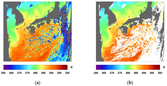
Figure 8. VIRR L1B 11 μm channel BT before and after cloud detection: (a) before cloud detection; (b) after cloud detection (The gray areas are the pixels exceeding the study area, land, and obviously cloud (pixels with the BT of 11 μm channel less than 260 K), the white areas are the pixels detected by Bayesian method as cloud).

2.4. SST Retrieval

The VIRR ${\mathrm{SST}}_{\mathrm{skin}}$ is retrieved using OE SST algorithm, and the principle of OE is shown in Equation (6) by Merchant et al. [24,35,36].

$$\widehat{z}=z\left(x_a\right)+{\left(K^T{S}_{\epsilon }^{-1}K+S_a^{-1}\right)}^{-1}{K}^T{S}_{\epsilon }^{-1}\left(y_0-F\left(x_a\right)\right)$$

(6)

where $\widehat{z}$ is a matrix with the retrieval results of ${\mathrm{SST}}_{\mathrm{skin}}$ and TCWV, $x_a$ is a matrix with the background ${\mathrm{SST}}_{\mathrm{skin}}$ and TCWV, $y_0$ is satellite observed BT, $F\left(x_a\right)$ is simulated BT calculated by atmospheric radiative modeling. K is a tangential vector, consisting of the partial derivative of the simulated BT to background ${\mathrm{SST}}_{\mathrm{skin}}$ and TCWV, $S_{\epsilon }$ is the covariance matrix of the satellite observed BT and the simulated BT, $S_a$ is the error of the background ${\mathrm{SST}}_{\mathrm{skin}}$ and TCWV. Figure 9 shows the retrieved VIRR ${\mathrm{SST}}_{\mathrm{skin}}$ in the daytime and nighttime on 28 March 2016.

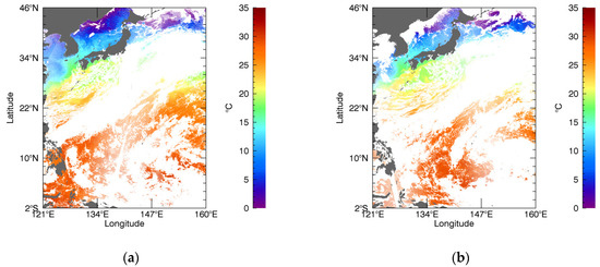
Figure 9. VIRR ${\mathrm{SST}}_{\mathrm{skin}}$ after projection in the daytime and nighttime on 28 March 2016: (a) daytime; (b) nighttime.

3. Results

We used high precision drifting buoy data, tropical moored buoy data, and high resolution drifter data of iQuam with a quality level of 5 to validate the retrieval results. The VIRR ${\mathrm{SST}}_{\mathrm{skin}}$ are matched with the buoy data. The temporal window is 1 h, the spatial window is 0.01° × 0.01°. To ensure the independence of matchups, when multiple VIRR ${\mathrm{SST}}_{\mathrm{skin}}\mathrm{s}$ or two buoy SSTs fall in the same grid, they are averaged. A total of 1807 matchups are obtained with a bias of −0.12 °C and a standard deviation of 0.52 °C, the correlation coefficient between VIRR ${\mathrm{SST}}_{\mathrm{skin}}$ and the buoy is 0.9960. The relationship between the VIRR ${\mathrm{SST}}_{\mathrm{skin}}$ and the buoy SST is shown in Figure 10. We can see that the VIRR ${\mathrm{SST}}_{\mathrm{skin}}$ is in good agreement with the buoy SST. The histogram of bias of VIRR ${\mathrm{SST}}_{\mathrm{skin}}$ with buoy SST is shown in Figure 11. It shows that the bias of most matchups is distributed near zero, and the numbers show a decreasing trend to both sides. Most points distribute between −1 °C and 1 °C. We calculate the distribution of bias; 322 matchups have bias within 0.1 °C, accounting for 18% of the total; 883 matchups have bias within 0.3 °C, accounting for 49% of the total; 1285 matchups have bias within 0.5 °C, accounting for 71% of the total; 1703 matchups have bias within 1 °C, accounting for 94% of the total. The presence of large numbers of negative and positive biases due to the influence of uncertainty of VIRR SST. However, the SST obtained by the OE is skin temperature, while the SST measured by the buoy is the bulk temperature. In a calm sea surface where the wind speed is less than 6 m/s, the skin temperature is about 0.17 °C lower than the bulk temperature [37], which is one of the reasons for negative bias. During the day, in the absence of strong winds to drive the vertical mixing of the water, the solar radiation can warm the sea surface water, which is one of the reasons for positive bias in the daytime [38]. There are more matchups on the left side of zero than on the right side, which means the skin effect leads to more negative bias pixels.

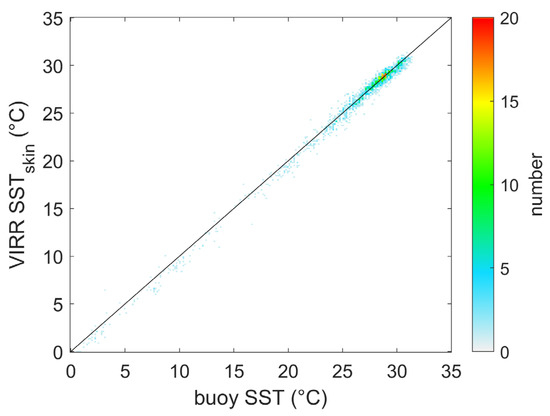
Figure 10. The relationship between the VIRR ${\mathrm{SST}}_{\mathrm{skin}}$ and the buoy SST.

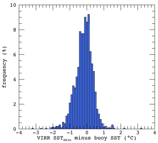
Figure 11. Histogram of bias of VIRR ${\mathrm{SST}}_{\mathrm{skin}}$ and buoy SST.

MetOp-A AVHRR ${\mathrm{SST}}_{\mathrm{skin}}$ from CCI project are used to evaluate the VIRR ${\mathrm{SST}}_{\mathrm{skin}}$. Since both the ${\mathrm{SST}}_{\mathrm{skin}}$ data are obtained by the OE are skin temperature, the descending nodes of the two satellites are close. The AVHRR ${\mathrm{SST}}_{\mathrm{skin}}$ with the highest quality and VIRR ${\mathrm{SST}}_{\mathrm{skin}}$ is projected on the grid of 0.04° × 0.04°. If multiple VIRR ${\mathrm{SST}}_{\mathrm{skin}}\mathrm{s}$ or AVHRR ${\mathrm{SST}}_{\mathrm{skin}}\mathrm{s}$ fall in the same grid, they will be averaged. The temporal window for matching between the VIRR ${\mathrm{SST}}_{\mathrm{skin}}$ and AVHRR ${\mathrm{SST}}_{\mathrm{skin}}$ is 1 h, and the spatial window is 0.04° × 0.04°. There are a total of 6,028,138 matchups between the VIRR ${\mathrm{SST}}_{\mathrm{skin}}$ and the AVHRR ${\mathrm{SST}}_{\mathrm{skin}}$, with a bias of 0.08 °C and a standard deviation of 0.55 °C. The correlation coefficient between VIRR ${\mathrm{SST}}_{\mathrm{skin}}$ and AVHRR ${\mathrm{SST}}_{\mathrm{skin}}$ is 0.9975. Figure 12 shows that the VIRR ${\mathrm{SST}}_{\mathrm{skin}}$ and the AVHRR ${\mathrm{SST}}_{\mathrm{skin}}$ have good consistency. The histogram of bias of VIRR ${\mathrm{SST}}_{\mathrm{skin}}$ with AVHRR ${\mathrm{SST}}_{\mathrm{skin}}$ is shown in Figure 13. It shows that the bias of most matchups is distributed near zero, decreasing to both sides. 16% of matchups are distributed within 0.1 °C, 45% of matchups are distributed within 0.3 °C, 67% of matchups are distributed within 0.5 °C, and 93% of matchups are distributed within 1 °C. The result is consistent with the validation result with the buoy. The number of matchups on the left and right of zero is roughly the same, which means that the skin effect does not need to be considered when comparing VIRR ${\mathrm{SST}}_{\mathrm{skin}}$ with AVHRR ${\mathrm{SST}}_{\mathrm{skin}}$.

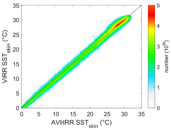
Figure 12. The relationship between the VIRR ${\mathrm{SST}}_{\mathrm{skin}}$ and the CCI AVHRR ${\mathrm{SST}}_{\mathrm{skin}}$.

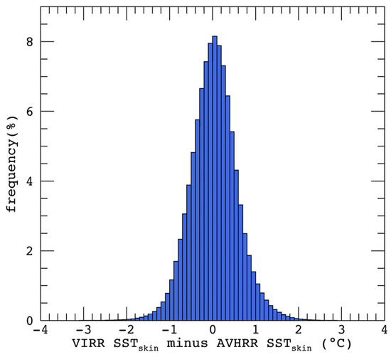
Figure 13. Histogram of bias of VIRR ${\mathrm{SST}}_{\mathrm{skin}}$ and CCI AVHRR ${\mathrm{SST}}_{\mathrm{skin}}$.

Due to the skin effect, the negative bias of VIRR ${\mathrm{SST}}_{\mathrm{skin}}$ and buoy includes the deviation of the skin temperature and the bulk temperature. The bias of the VIRR ${\mathrm{SST}}_{\mathrm{skin}}$ and the AVHRR ${\mathrm{SST}}_{\mathrm{skin}}$ is close to 0, and the standard deviation is close to the standard deviation from the buoy, indicating that the validation results compared with AVHRR ${\mathrm{SST}}_{\mathrm{skin}}$ and buoy SST are consistent.

The bias of the OE SST retrieval is mainly caused by the difference between the satellite observation BT and the simulated BT, the background skin temperature error, and the modeling error. Prior to the retrieval, inter-calibration with MODIS L1B data was first carried out. The Bayesian cloud detection and SST retrieval are performed with the calibration results, which contributed to the accuracy of the retrieval results. In addition, during the retrieval process, the resolution of the background field data is lower than the resolution of the satellite data, which causes the retrievals to be smoothed, thus the accuracy at the temperature front may be affected. We hope to work to improve this situation in future research.

4. Discussion

Since the BTs of the pixels in cloud conditions are low, the SST contaminated by the cloud is obviously low. Thus, it can be judged as to whether there is a cloud missed in detection by checking the SST values. In Section 3, the bias between VIRR ${\mathrm{SST}}_{\mathrm{skin}}$ and the buoy is −0.12 °C, which indicates the skin effect. The bias of VIRR ${\mathrm{SST}}_{\mathrm{skin}}$ and AVHRR ${\mathrm{SST}}_{\mathrm{skin}}$ is 0.08 °C. Since VIRR ${\mathrm{SST}}_{\mathrm{skin}}$ compared with the highest-level AVHRR ${\mathrm{SST}}_{\mathrm{skin}}$, the time window is 1 h, so the influence of cloud is minimized when the two are matched. In order to further evaluate the validity of cloud detection, the VIRR and AVHRR monthly mean ${\mathrm{SST}}_{\mathrm{skin}}$ are calculated, respectively. Firstly, the daily daytime and nighttime VIRR ${\mathrm{SST}}_{\mathrm{skin}}$ are averaged to obtain monthly daytime and nighttime mean ${\mathrm{SST}}_{\mathrm{skin}}$, respectively. When multiple points fall into the same grid, the average is calculated. Next, the monthly daytime and nighttime mean ${\mathrm{SST}}_{\mathrm{skin}}$ are averaged to obtain VIRR monthly mean ${\mathrm{SST}}_{\mathrm{skin}}$. The VIRR monthly mean ${\mathrm{SST}}_{\mathrm{skin}}$ of March, May, August, and November are shown in Figure 14, and the AVHRR monthly mean ${\mathrm{SST}}_{\mathrm{skin}}$ are also obtained in the same way. The difference between VIRR and AVHRR monthly mean ${\mathrm{SST}}_{\mathrm{skin}}$ is calculated. The bias is 0.07 °C, the standard deviation is 0.45 °C, and the correlation coefficient is 0.9976. The bias is close to 0, and there are no more negative bias pixels in VIRR ${\mathrm{SST}}_{\mathrm{skin}}$. Therefore, it demonstrates the validity of the cloud detection, i.e., there are no obvious cloud missing pixels.

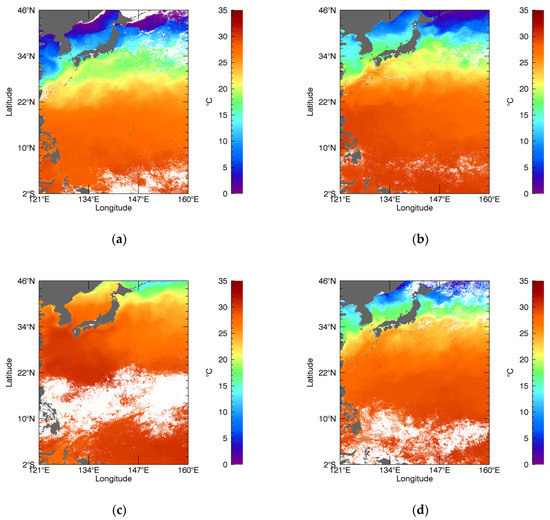
Figure 14. The VIRR monthly mean ${\mathrm{SST}}_{\mathrm{skin}}$ of March, May, August, and November: (a) March; (b) May; (c) August; (d) November.

5. Conclusions

The skin SST is received from FY-3C/VIRR. Firstly, the FY-3C/VIRR BTs are inter-calibrated with the Terra/MODIS after removing the spectral difference. After inter-calibration, the BT difference between the two after removing the spectral difference is close to zero. Next, the Bayesian cloud detection and OE algorithm are applied to detect cloud pixel and retrieve ${\mathrm{SST}}_{\mathrm{skin}}$ using the calibrated BTs. Comparing the retrieval results with the buoy SST, the bias is −0.12 °C, and the standard deviation is 0.52 °C. The VIRR ${\mathrm{SST}}_{\mathrm{skin}}$ is also compared with MetOp-A CCI AVHRR ${\mathrm{SST}}_{\mathrm{skin}}$, the bias is 0.08 °C, and the standard deviation is 0.55 °C. The results compared with CCI AVHRR ${\mathrm{SST}}_{\mathrm{skin}}$ and buoy SST are consistent considering the difference of skin and bulk temperature. In this study, only data from the Western Pacific are used for testing. The method can be further applied to global ${\mathrm{SST}}_{\mathrm{skin}}$ retrieval from FY-3C/VIRR.

References

- Barnett, T.P.; Graham, N.; Pazan, S.; White, W.; Latif, M.; Flügel, M. ENSO and ENSO-related Predictability. Part I: Prediction of Equatorial Pacific Sea Surface Temperature with a Hybrid Coupled Ocean–Atmosphere Model. J. Clim. 1993, 6, 1545–1566. [Google Scholar] [CrossRef] [Green Version]
- Dai, A. Future Warming Patterns Linked to Today’s Climate Variability. Sci. Rep. 2016, 6, 19110. [Google Scholar] [CrossRef] [PubMed] [Green Version]
- Ward, M.N.; Folland, C.K. Prediction of seasonal rainfall in the north nordeste of Brazil using eigenvectors of sea-surface temperature. Int. J. Climatol. 1991, 11, 711–743. [Google Scholar] [CrossRef]
- Aydoğdu, A.; Pinardi, N.; Pistoia, J.; Martinelli, M.; Belardinelli, A.; Sparnocchia, S. Assimilation experiments for the Fishery Observing System in the Adriatic Sea. J. Mar. Syst. 2016, 162, 126–136. [Google Scholar] [CrossRef]
- Harries, J.E.; Llewellyn-Jones, D.T.; Minnett, P.J.; Saunders, R.W.; Zavody, A.M.; Wadhams, P.; Taylor, P.K.; Houghton, J.T. Observations of Sea-Surface Temperature for Climate Research and Discussion. Philos. Trans. R. Soc. A Math. Phys. Eng. Sci. 1983, 309, 381–395. [Google Scholar]
- Ohring, G.; Wielicki, B.; Spencer, R. Satellite Instrument Calibration for Measuring Global Climate Change: Report of a Workshop. Bull. Am. Meteorol. Soc. 2004, 86, 1303–1313. [Google Scholar] [CrossRef]
- Casey, K.S.; Brandon, T.B.; Cornillon, P.; Evans, R. The Past, Present, and Future of the AVHRR Pathfinder SST Program. In Oceanography from Space; Springer: Dordrecht, The Netherland, 2010; pp. 273–287. [Google Scholar] [CrossRef]
- Borgne, P.L.; Legendre, G.; Marsouin, A. Operational SST Retrieval from Metop/AVHRR. In Proceedings of the 2007 EUMETSAT Conference, Amsterdam, The Netherlands, 24–28 September 2007. [Google Scholar]
- Minnett, P.J.; Brown, O.B.; Evans, R.H.; Key, E.L.; Kearns, E.J.; Kilpatrick, K.; Kumar, A.; Maillet, K.A.; Szczodrak, G. Sea-surface temperature measurements from the Moderate-Resolution Imaging Spectroradiometer (MODIS) on Aqua and Terra. In Proceedings of the IEEE International Geoscience & Remote Sensing Symposium, Anchorage, AK, USA, 20–24 September 2004. [Google Scholar]
- Gentemann, C.L. Three way validation of MODIS and AMSR-E sea surface temperatures. J. Geophys. Res. Ocean. 2014, 119, 2583–2598. [Google Scholar] [CrossRef]
- Godin, R. Joint Polar Satellite System (JPSS) Operational Algorithm Description (OAD) Document for VIIRS Sea Surface Temperature (SST) Environmental Data Record (EDR) Software; National Polar-Orbiting Operational Environmental Satellite System: Washington, DC, USA, 2017. [Google Scholar]
- Dash, P.; Ignatov, A.; Kihai, Y.; Sapper, J. The SST quality monitor (SQUAM). J. Atmos. Ocean. Technol. 2010, 27, 1899–1917. [Google Scholar] [CrossRef]
- Petrenko, B.; Ignatov, A.; Kihai, Y.; Stroup, J.; Dash, P. Evaluation and selection of SST regression algorithms for JPSS VIIRS. J. Geophys. Res. Atmos. 2014, 119, 4580–4599. [Google Scholar] [CrossRef]
- Tsamalis, C.; Saunders, R. Quality Assessment of Sea Surface Temperature from ATSRs of the Climate Change Initiative (Phase 1). Remote Sens. 2018, 10, 497. [Google Scholar] [CrossRef] [Green Version]
- Luo, B.; Minnett, P.J.; Szczodrak, M.; Kilpatrick, K.; Izaguirre, M. Validation of Sentinel-3A SLSTR derived Sea-Surface Skin Temperatures with those of the shipborne M-AERI. Remote Sens. Environ. 2020, 244, 111826. [Google Scholar] [CrossRef]
- Martin, S. An Introduction to Ocean Remote Sensing; Cambridge University Press: Cambridge, UK, 2014; p. 8. [Google Scholar]
- Wang, S.; Cui, P.; Zhang, P.; Ran, M.; Lu, F.; Wang, W. FY-3C/VIRR SST algorithm and cal/val activities at NSMC/CMA. SPIE Proc. 2014, 9261, 92610G. [Google Scholar] [CrossRef]
- Wang, S.J.; Cui, P.; Zhang, P.; Yang, Z.D.; Ran, M.N.; Xiu-Qing, H.U.; Feng, L.U.; Liu, J. Progress of VIRR Sea Surface Temperature Product of FY-3 Satellite. Aerospace Shanghai 2017, 34, 79–84. [Google Scholar]
- Wang, S.J.; Cui, P.; Zhang, P.; Yang, Z.D.; Xiu-Qing, H.U.; Ran, M.N.; Liu, J.; Lin, M.Y.; Qiu, H. FY-3C/VIRR SST Sea Surface Temperature Products and Quality Validation. J. Appl. Meteorol. Sci. 2020, 31, 729–739. [Google Scholar] [CrossRef]
- Yang, H.; Wang, S.J.; Liu, M.K.; Guan, L. Evaluation of sea surface temperature from FY-3C/VIRR observations in the Northwest Pacific. Period. Ocean. China 2020, 50, 151–159. [Google Scholar] [CrossRef]
- Wong, E.W.; Minnett, P.J. The Response of the Ocean Thermal Skin Layer to Variations in Incident Infrared Radiation. J. Geophys. Res. Ocean. 2018, 123, 2475–2493. [Google Scholar] [CrossRef]
- Soloviev, A.V.; Lukas, R. The Near-Surface Layer of the Ocean: Structure, Dynamics, and Applications, 2nd ed.; Springer: Dordrecht, The Netherland, 2014; p. 71. [Google Scholar]
- Minnett, P.J.; Kaiser-Weiss, A.K. Group for High Resolution Sea-Surface Temperature Discussion Document: Near-Surface Oceanic Temperature Gradients. 2012. Available online: https://www.ghrsst.org/wp-content/uploads/2021/04/SSTDefinitionsDiscussion.pdf (accessed on 6 September 2020).
- Merchant, C.J.; Le Borgne, P.; Marsouin, A.; Roquet, H. Optimal estimation of sea surface temperature from split-window observations. Remote Sens. Environ. 2008, 112, 2469–2484. [Google Scholar] [CrossRef]
- Fengyun Satellite Remote Sensing Data Service Network. Available online: http://satellite.nsmc.org.cn/PortalSite/StaticContent/DeviceIntro_FY3_VIRR.aspx (accessed on 13 February 2019).
- NASA MODIS. Available online: https://modis.gsfc.nasa.gov/about/specifications.php (accessed on 6 June 2020).
- Merchant, C.J.; Embury, O.; Bulgin, C.E.; Block, T.; Corlett, G.K.; Fiedler, E.; Good, S.A.; Mittaz, J.; Rayner, N.A.; Berry, D.; et al. Satellite-based time-series of sea-surface temperature since 1981 for climate applications. Sci. Data 2019, 6, 223. [Google Scholar] [CrossRef] [Green Version]
- Xu, F.; Ignatov, A. In situ SST Quality Monitor (iQuam). J. Atmos. Ocean. Technol. 2014, 31, 164–180. [Google Scholar] [CrossRef]
- Berrisford, P.; Dee, D.P.; Fielding, M.; Fuentes, M.; Kållberg, P.W.; Kobayashi, S.; Uppala, S. The ERA-Interim Archive; ECMWF: Reading, UK, 2009; p. 16. [Google Scholar]
- Xiong, X.; Chiang, K.; Sun, J.; Barnes, W.L.; Guenther, B.; Salomonson, V.V. NASA EOS Terra and Aqua MODIS on-orbit performance. Adv. Space Res. 2009, 43, 413–422. [Google Scholar] [CrossRef]
- Qin, Y.; McVicar, T.R. Spectral band unification and inter-calibration of Himawari AHI with MODIS and VIIRS: Constructing virtual dual-view remote sensors from geostationary and low-Earth-orbiting sensors. Remote Sens. Environ. 2018, 209, 540–550. [Google Scholar] [CrossRef]
- Voss, S.; Merchant, C.; Maccallum, S. Generalized Bayesian Cloud Screening (GBCS); School of Geosciences: Edinburgh, UK, 2008. [Google Scholar]
- SST CCI Auxiliary Datasets. Available online: https://zenodo.org/record/2586714#.YGWWWa8zaUk (accessed on 7 April 2021).
- Merchant, C.J.; Harris, A.R.; Maturi, E.; Maccallum, S. Probabilistic physically based cloud screening of satellite infrared imagery for operational sea surface temperature retrieval. Q. J. R. Meteorol. Soc. 2005, 131, 2735–2755. [Google Scholar] [CrossRef] [Green Version]
- Merchant, C.J.; Le Borgne, P.; Roquet, H.; Marsouin, A. Sea surface temperature from a geostationary satellite by optimal estimation. Remote Sens. Environ. 2009, 113, 445–457. [Google Scholar] [CrossRef]
- Merchant, C.J.; Le Borgne, P.; Roquet, H.; Legendre, G. Extended optimal estimation techniques for sea surface temperature from the Spinning Enhanced Visible and Infra-Red Imager (SEVIRI). Remote Sens. Environ. 2013, 131, 287–297. [Google Scholar] [CrossRef]
- Donlon, C.; Minnett, P.; Gentemann, C.; Nightingale, T.; Barton, I.; Ward, B.; Murray, J. Toward Improved Validation of Satellite Sea Surface Skin Temperature Measurements for Climate Research. J. Clim. 2002, 14, 353–369. [Google Scholar] [CrossRef] [Green Version]
- Minnett, P.J.; Alvera-Azcárate, A.; Chin, T.M. Half a century of satellite remote sensing of sea-surface temperature. Remote Sens. Environ. 2019, 233, 111366. [Google Scholar] [CrossRef]
Publisher’s Note: MDPI stays neutral with regard to jurisdictional claims in published maps and institutional affiliations. |
© 2022 by the authors. Licensee MDPI, Basel, Switzerland. This article is an open access article distributed under the terms and conditions of the Creative Commons Attribution (CC BY) license (https://creativecommons.org/licenses/by/4.0/).