Article

A Simple Statistical Intra-Seasonal Prediction Model for Sea Surface Variables Utilizing Satellite Remote Sensing

1
School of Marine Science and Technology, Tianjin University, Tianjin 300072, China
2
Tianjin Key Laboratory for Oceanic Meteorology, Tianjin 300074, China
3
The PLA 31010 Units, Beijing 100081, China
4
Tianjin Institute of Meteorological Sciences, Tianjin 300074, China
*
Author to whom correspondence should be addressed.
Remote Sens. 2022, 14(5), 1162; https://doi.org/10.3390/rs14051162
Submission received: 18 December 2021 / Revised: 21 February 2022 / Accepted: 24 February 2022 / Published: 26 February 2022
(This article belongs to the Section Ocean Remote Sensing)

Abstract

:
In this paper, a novel and simple statistical prediction model for sea surface multivariate is developed based on extended empirical orthogonal functions (referred to as the MEEOF model). This simple model embeds the temporal evolution information into the empirical orthogonal function spatial patterns, which effectively captures the spatial distribution of the sea surface variables and their evolution process over time, and can be used to improve the accuracy of intra-seasonal ocean forecasts. At the same time, it considers both the correlation between different spatial and temporal points and the dynamic balance between different sea surface variables. The performance of the MEEOF prediction model has been examined in the South China Sea (SCS) based on remote sensing satellite datasets. Experimental results demonstrate that this model has significant forecasting capability within the forecast window of 15–90 days, compared with the traditional persistence forecasts and optimal climatic normal (OCN) results. Furthermore, this model exhibits good forecast performance throughout the entire forecast window; the final prediction model (referred to as the fusion model) is established by obtaining the weighted average for the MEEOF forecasts and persistence forecast results. Numerical experimental results show that this fusion prediction model consistently outperforms the persistence model, the OCN model, and the linear regression model over the entire forecast window. A case study shows that the propagation of ocean waves and the coordination between different sea surface variables can be well predicted by this simple model, indicating that this fusion model has a potential advantage in intra-seasonal predictions of the ocean.

1. Introduction

Ocean forecasting is based on the understanding of the past and present state of the ocean and its evolutionary laws, using numerical models, observational data, data assimilation schemes, and other statistical methods to analyze, judge, and forecast ocean processes and phenomena [1]. It is well known that accurate predictions of the ocean state at different spatial and temporal scales are necessary [2]. In particular, mesoscale phenomena are widespread throughout the ocean, where mesoscale eddies are the most energetic forms of motion prevailing in the ocean [3].
The South China Sea (SCS) is one of the largest marginal seas, exhibiting complex topography [4]. On the one hand, the SCS has abundant water exchange channels and is vulnerable to the large-scale circulation of the Sulu Sea and the Pacific Ocean, showing strong seasonal signals and inter-annual oscillations [5]; on the other hand, the unique geographical environment of the SCS makes it extremely abundant in oceanic eddies, and mesoscale fluctuations on the temporal-spatial scales of between 20–150 days and 50–500 km dominate the oceanic variability [6]. In view of this, It is essential to predict the intra-seasonal variation of these mesoscale signals.
Generally, there are two main types of methods for forecasting ocean variables [7]. One is based on the numerical model, which achieves the forecasting of ocean variables through the use of ocean dynamics models [8,9,10,11]; the other is a data-driven model. Ocean numerical models use various evolution equations to describe ocean variability [12]. With the rapid development of ocean data assimilation schemes and the improvement of model resolution, numerical model forecasting technology has been increasingly developed and has become an important approach for prediction. The Global National Real-Time Ocean Forecasting System (RTOFS), which is based on the Hybrid Coordinate Ocean Model (HYCOM) [10], is the most widely used operational forecasting system, and it can provide daily forecasts for eight days [13]. The National Earth System Prediction Capability (ESPC) forecasting system is also based on the HYCOM, and it is a fully coupled forecasting system with a spatial resolution of 1/25, providing 16-day daily forecasts and 45-day weekly forecasts [14]. Also, the French Mercator Ocean International forecast system uses the Nucleus for European Modeling of the Ocean (NEMO) to predict sea level for 10 days in advance [15]. For some special and long-term oceanic phenomena, such as the western boundary currents, in the case of known external forcing, its predictability can be within a few months [16]. However, the numerical models mentioned above involve a large number of ideal assumptions and also require complex computational platforms [17,18].
With the development of ocean satellite observations and ocean data assimilation technologies, a large amount of marine environmental data has been accumulated, including in situ observation data, satellite remote sensing data, and high-quality reanalysis products. These data provide strong support for us to carry out ocean forecasting based on data-driven methods. Data-driven forecasting methods often use statistical tools or artificial intelligence methods to analyze large amounts of historical data and find the potential connections between the data. Such methods are suitable for the prediction of physical processes that are not clearly defined. Common statistical methods and machine learning methods are data-driven models. Recently, the research topic of the data-driven forecasting of ocean variables has received increasing attention [19,20,21], especially in the context of the limited understanding of ocean processes. Neural network models, such as multilayer perceptron (MLP) and long- and short-term memory (LSTM) models, have been used to predict sea surface temperature (SST) [22,23]; Imani, et al. [24] analyzed and predicted monthly sea level anomalies (SLAs) using an autoregressive integrated moving averaged (ARIMA) model; a linear regression model combining the dynamical ENSO was used to predict the SST in the Indian Ocean [19]; an efficient neural network has been used to predict SST for several sites [25]. However, we learn from the above studies that traditional data-driven methods usually describe the ocean state at a single scale, ignoring the interactions between different variables and the multi-scale effects of the ocean. Therefore, they are only suitable for the short-term forecasting of ocean variables. For traditional linear statistical models, tangent linear models are generally considered, which cannot resolve nonlinear signals and therefore, cannot extend the time validity of predictions; while for nonlinear models such as neural networks, such approaches generally do not consider the relationship between different variables and cannot explain their dependence over longer periods.
Considering the above, we develop a simple statistical prediction model based on the multivariate extended empirical orthogonal function (EEOF) decomposition, which is referred to as the MEEOF prediction model in this study. With the EEOF analysis, the maximum probable and orthogonal evolution patterns of the ocean can be extracted from the various possible evolutionary forms in the past; in addition, multiscale, spatiotemporal information, as well as the correlation information between different variables, are all integrated into the patterns, and those patterns are coherent both in space and time. The orthogonal patterns obtained in this way contain both the temporal evolution of a certain variable and the dynamic correlation between different variables. Then, the future predictions are achieved by projecting the current state onto these patterns to obtain the weight coefficients. This model transforms the spatiotemporal prediction problem into a series of linear combinations of basis functions and optimal weight coefficients, taking into account the fluctuations of the ocean. Our “test block” of the ocean is the SCS, which is a semi-enclosed basin [26,27].
The remaining sections of this paper are organized as follows: Satellite remote sensing observations data and the study area in this study are described in Section 2; the related methodology is also presented in this section. In Section 3, experiments and the corresponding results are given in detail. Then, in Section 4, we develop a fusion model to enable satisfactory performance throughout the entire forecast window. The discussion is included in Section 5. Finally, we summarize the conclusions in Section 6.

2. Observations and Prediction Model

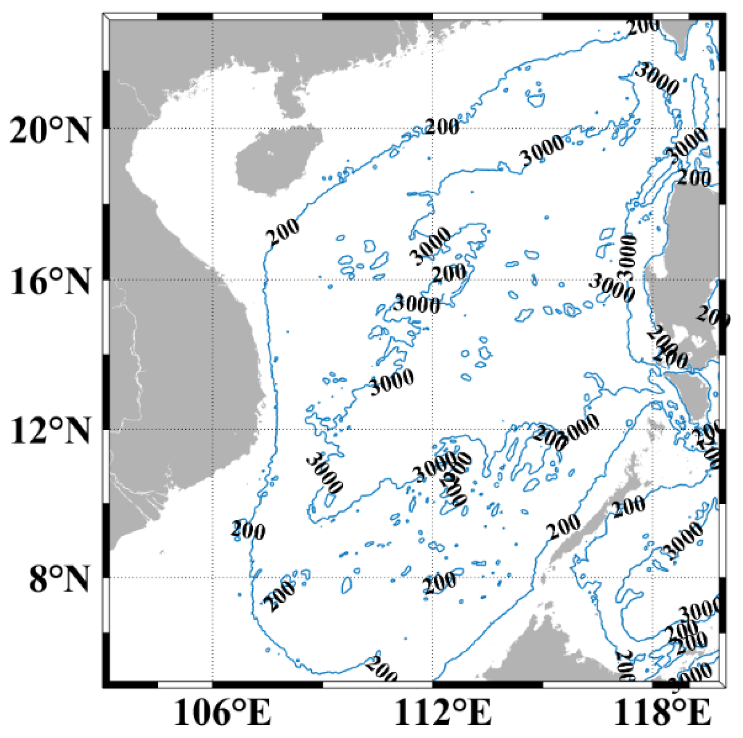
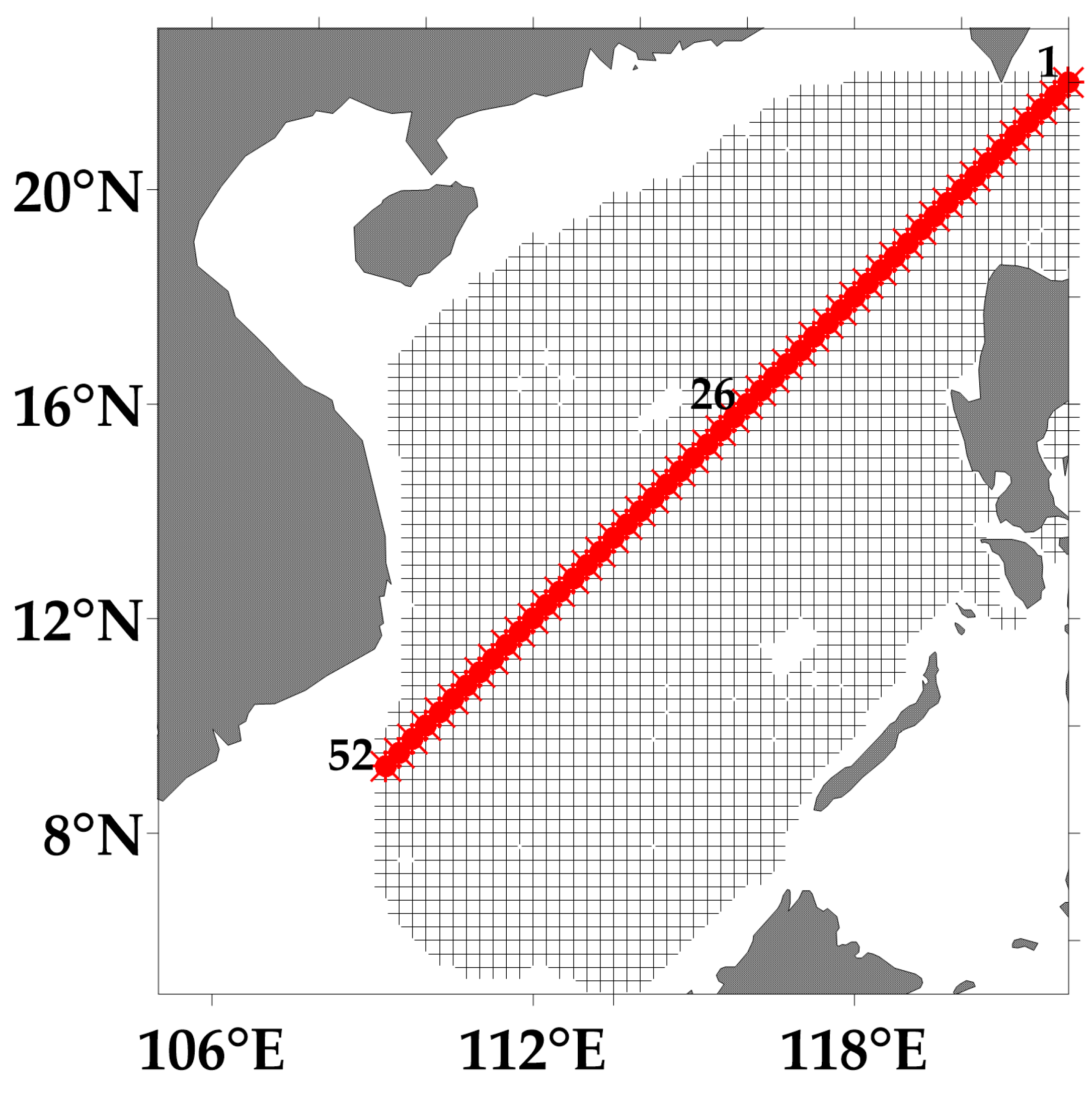
2.1. Data Collection

In this study, considering the correlation of different variables and the availability of current ocean satellite remote sensing data, we chose SLA and SST for modeling. The SLA data used here is released by the Copernicus Marine Environment Monitoring Service (CMEMS) with a spatial resolution of 1/4° and a temporal resolution of 1 day. This data is a multi-satellite fused altimetry data that provides daily SLA values from 1 January 1993 to the present. The SST data is produced by the National Oceanic and Atmospheric Administration (NOAA) daily Optimum Interpolation Sea Surface Temperature (daily OISST, version 2) with a spatial resolution of 1/4°. The AVHRR-Only SSTs data are used here, which use only satellite SSTs from the AVHRR and provide daily SST values from 1 September 1981 to the present [28].
The latitude and longitude of the study area ranges from 5° N to 23° N and 105° E to 122° E, respectively, as shown in Figure 1. Moreover, since the following modeling process involves orthogonal decomposition, we hope that the patterns obtained from the decomposition are not only the maximum probable results, but also the optimal spectral decomposition results [29]. Based on the above aims, the Sulu Sea is excluded in this study by temporarily disregarding the interaction between the Sulu Sea and the SCS. In addition, in the shore and shallow areas, the satellite remote sensing data are susceptible to tidal and internal waves that can lead to accuracy degradation [30]. Thus, these data are masked out in this study.
Given the availability and time frame of the aforementioned remote sensing dataset, the 26-year data from 1993 to 2018 are selected as the study dataset. To ensure that the experiments are statistically significant, as well as to guarantee the reliability of the experimental results, a round-robin approach is adopted, i.e., any set of 25 years of data is used to establish each prediction model, while another one-year set of data serves as the independent variable to validate the performance of the prediction model. Here, the spatial-temporal grids for the analysis and prediction are set up with the spatial resolution of 0.25° × 0.25° and the temporal resolution of 1 day, respectively. In this study, we can regard them as true fields.

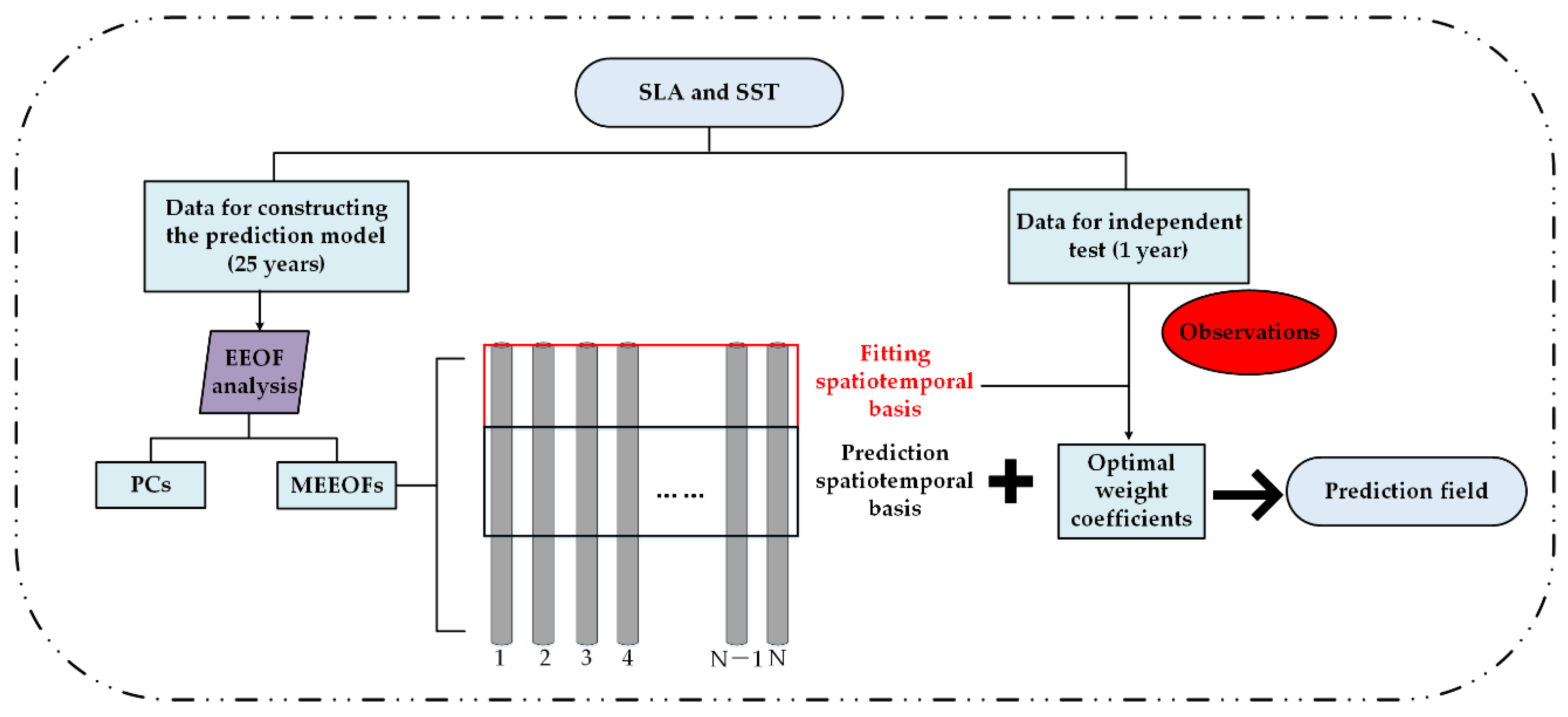
2.2. Description of the Proposed Prediction Model

The flowchart of the proposed prediction model is shown in Figure 2. In the model construction process, the multivariate dataset is divided into two parts, one with 25 years of data for constructing the prediction model, and the other with 1 year of data for validating. Then, EEOF analysis is performed on these 25 years of data, and the multivariate extended orthogonal spatiotemporal modes (MEEOFs, Appendix A) and the corresponding principal components (PCs) can be obtained. The details are described in Section 2.3.
At the time of prediction, a certain proportion of MEEOFs are retained based on the significant test results [31] and divided into two parts: the fitting spatiotemporal basis and the prediction spatiotemporal basis. The weight coefficients can be obtained by projecting the observational data from the independent test sample onto the fitting spatiotemporal basis; then, this set of optimal weight coefficients can be combined with the prediction spatiotemporal basis to obtain the final prediction field. The details are explained in Section 2.4.

2.3. Extended Empirical Orthogonal Function Analysis of Multivariate Observations

Empirical orthogonal function (EOF) analysis is a classical statistical method in the field of the atmosphere and the ocean [32]. It can quickly decompose a large amount of data and extract the main spatial structure, effectively analyzing the spatial and temporal variability of the data field while reducing dimensionality [33,34,35]. However, it cannot describe the evolution of spatial features in the time dimension, which makes it impossible for us to understand its spatial variation using a long-time scale. Therefore, to solve this problem, heterogeneous datasets at different times could be used in EOF analysis, which is called EEOF analysis [36,37]. In this way, the variation of the variable over continuous time can be considered. Therefore, EEOF analysis has been widely used to study the long-term evolution of atmospheric and oceanic processes [38].
In this study, the window length is 1 year, i.e., the column vector consisting of the daily data from 1 January to 31 December of each year represent one subsample for EEOF analysis. EEOF analysis is also performed on the multiple sea surface variables simultaneously, and Z represents the original sample matrix.
Z = [ Z 1 Z m Z M ]
In this matrix, Z m represents the m th subsample, and can be expressed as follows:
Z m = [ Z S L A m , 1 Z S S T m , 1 Z S L A m , k Z S S T m , k Z S L A m , 365 Z S S T m , 365 ]
where Z S L A m , k , ( m = 1 , 2 , , M ;   k = 1 , 2 , , 365 ) represents the remote sensing data of SLA at the kth day for the mth subsample. Here, Z S L A m , k is a column vector with the dimensions of N s × 1 , and N s is the number of grid points in one day of SLA. Therefore, the dimensions of (1) are N × M , where N = N s × 365 × 2 is the total dimension of one subsample, and M is the number of the subsamples. Apparently, N M here.
By arranging the matrix in this way, each column vector contains the signal over a period of time, and also expresses the spatiotemporal multiscale details of the sea surface variables. At the same time, the simultaneous decomposition of multiple variables can take into account the dynamics and thermal matching relationships between different variables.
In this study, EEOF decomposition is applied to the anomaly matrix, which is constructed by removing the climatology. Climatology usually represents the periodic signals of the ocean [39], and here, we assume that
Z ¯ S L A k = 1 M m = 1 M Z S L A m , k , Z ¯ S S T k = 1 M m = 1 M Z S S T m , k
and climatology can be expressed as
Z ¯ = [ Z ¯ S L A 1 Z ¯ S L A 1 Z ¯ S L A 1 Z ¯ S S T 1 Z ¯ S S T 1 Z ¯ S S T 1 Z ¯ S L A k Z ¯ S L A k Z ¯ S L A k Z ¯ S S T k Z ¯ S S T k Z ¯ S S T k Z ¯ S L A 365 Z ¯ S L A 365 Z ¯ S L A 365 Z ¯ S S T 365 Z ¯ S S T 365 Z ¯ S S T 365 ]
Therefore,
Z a n o m a l y = Z Z ¯
where Z a n o m a l y is the anomaly matrix.
In addition, the matrix (5) needs to be standardized, since the scales and units differ between different variables:
Z ˜ σ 1 Z a n o m a l y
where Z ˜ is the matrix for EEOF decomposition, and σ is the standardization matrix,
σ = d i a g [ , σ Z p k , ]
σ Z p k = 1 M m = 1 M [ Z p m , k Z ¯ p k ] 2
where Z p m , k represents the remote sensing data of the p th sea surface variable at k th day for the m th subsample, and p = 1 , 2 corresponds to SLA and SST, respectively.
From now on, the purpose of this step is to decompose Z ˜ into the orthogonal modes V 1 and the corresponding principal components T 1 , i.e., Z ˜ = V 1 T 1 , where the dimensions of V 1 and T 1 are N × N and N × M , respectively. The correlation coefficient matrix should be constructed as follows:
C o r ( Z ˜ ) 1 M Z ˜ Z ˜ T
Here, C o r ( Z ˜ ) effectively takes into account not only the temporal and spatial correlation between different points, but also the dynamic balance of the different sea surface variables.
In general, we need to perform Jacobian decomposition on C o r ( Z ˜ ) . However, as mentioned before, N M in this study, and the dimensions of C o r ( Z ˜ ) , are too large to be allocated in the computer memory. Fortunately, Z ˜ Z ˜ T and Ζ ˜ T Z ˜ have the same nonzero eigenvalues, although their eigenvectors differ. Thus, the Jacobian decomposition would apply to the matrix Ζ ˜ T Z ˜ here to reduce the computational cost,
Z ˜ T Z ˜ V 2 = V 2 Λ
where V 2 denotes the eigenvector of Ζ ˜ T Z ˜ , Λ is a diagonal matrix, and the elements on the diagonal represent the eigenvalues,
Λ = ( λ 1 0 0 0 λ 2 0 0 0 λ M )
Then multiply Z ˜ to each side of the Equation (10)
Z ˜ Z ˜ T Z ˜ V 2 = Z ˜ V 2 Λ
We found that Z ˜ V 2 is the eigenvector of C o r ( Z ˜ ) , with Λ being the eigenvalue matrix. Assume that
V 1 = ( V 1 m a i n V 1 r e s i d u a l )
where V 1 m a i n is the dominant part of V 1 . We can find that the relationship between V 1 m a i n and V 2 can be written as follows:
V 1 m a i n = 1 Λ Z ˜ V 2
Thus, T 1 m a i n = ( V 1 m a i n ) T Z ˜ where the dimensions of V 1 m a i n and T 1 m a i n are N × M and M × M , respectively. Finally, the original matrix Z can be expressed as follows:
Z = Z ¯ + σ Z ˜ = Z ¯ + σ V 1 m a i n T 1 m a i n
So far, the anomaly data of the sea surface multivariate are decomposed into MEEOFs and corresponding PCs in this way. Notably, MEEOFs here contain not only the temporal evolution information of a certain variable, but also the spatial relationship between different sea surface variables. Therefore, this provides effectual information for the prediction of the sea surface multivariate.

2.4. Multivariate Prediction

When enough samples are available, we can assume that the ocean has gone through enough possible initial states and has evolved in all possible initial states to provide information for predicting future state. In this sense, if the ocean state at the current moment has some similarity to the state at some point in the past, then the future evolutionary form can be determined based on the past evolutionary form. In this study, MEEOF analysis extracts the most likely orthogonal eigen evolution from the various possible evolution forms in the past.
Therefore, if a sufficiently large number of samples are used, more MEEOFs can be obtained by decomposition, allowing a more complete phase space to explain the sea surface processes represented by SLA and SST. By projecting the observations onto these MEEOFs, the optimal weight coefficients can be obtained; then, the spatiotemporal prediction can be achieved by combining these weight coefficients with the prediction spatiotemporal basis. Here, MEEOFs V 1 m a i n from the EEOF analysis can be divided into two parts,
V 1 m a i n = ( V f i t t i n g V p r e d i c t i o n )
where V f i t t i n g is the spatiotemporal basis used for fitting the observation data and V p r e d i c t i o n is the basis for the prediction. Similarly, the standardization matrix σ can also be divided into the following form:
σ = ( σ f i t t i n g 0 0 σ p r e d i c t i o n )
Climatology can also be divided into two parts, that is,
Z ¯ = ( Z ¯ f i t t i n g Z ¯ p r e d i c t i o n )
If the observational data Z o b s is known for a certain period of time, we can obtain the corresponding coefficients T o p t i m a l using the least squares estimation (LSE) approach, and the cost function J can be constructed as follows:
J ( Τ o p t i m a l ) = 1 2 ( Z ¯ f i t t i n g + σ f i t t i n g V f i t t i n g T o p t i m a l Z o b s ) T ( Z ¯ f i t t i n g + σ f i t t i n g V f i t t i n g T o p t i m a l Z o b s )
By making the gradient of the cost function J be zero, that is
0 = T o p t i m a l J ( T o p t i m a l )
we can find
T o p t i m a l = ( V f i t t i n g T σ f i t t i n g 2 V f i t t i n g ) 1 V f i t t i n g T σ f i t t i n g ( Z o b s Z ¯ f i t t i n g )
Then, based on the optimal weight coefficients T o p t i m a l obtained above and the prediction spatiotemporal basis V p r e d i c t i o n , the prediction results can be expressed as:
Z p r e d i c t i n = Z ¯ p r e d i c t i o n + σ p r e d i c t i o n V p r e d i c t i o n T o p t i m a l

3. Experimental Results

3.1. Performance Evaluation Criteria

In this study, a round-robin experiment is conducted on the original dataset of the 26-year period in the SCS: in each experiment, the datasets with 25 years are used as the samples for EEOF decomposition; then, another independent year is used for prediction validation. For each independent year, we conduct 200 prediction tests, thus a total of 5200 tests are conducted for 26 trails. With a spatial resolution of 0.25° × 0.25°, the total number of spatial grid points of SLA and SST over the entire study area for 1 year is 1,679,730, and the total number of samples is 25. The statistical metrics of the mean absolute error (MAE), root mean square error (RMSE), and correlation coefficient (CC) are used to assess the accuracy of the prediction. In this study, MAE and RMSE for ith grid point can be expressed as follows:
M A E i = ( j = 1 M t e s t | O B S i j P R E i j | ) / M t e s t
R M S E i = j = 1 M t e s t ( O B S i j P R E i j ) 2 M t e s t
The spatial-temporal averaged CC can be expressed as:
C C = [ j = 1 M t e s t i = 1 N N ( O B S i j O B S ¯ ) ( P R E i j P R E ¯ ) j = 1 M t e s t i = 1 N N ( O B S i j O B S ¯ ) 2 ( P R E i j P R E ¯ ) 2 ] / ( N N × M t e s t ) { O B S ¯ = [ j = 1 M t e s t ( i = 1 N N O B S i j ) ] / ( N N × M t e s t ) , P R E ¯ = [ j = 1 M t e s t ( i = 1 N N P R E i j ) ] / ( N N × M t e s t ) }
where O B S i j and P R E i j are represent the observation (true) value and prediction value of the i th grid point in the j th validation sample; N N is the number of spatial grid points and M t e s t represents the number of validation samples.

3.2. Code Performance

In this section, experiments are carried out to test the code performance of the EEOF decomposition, since it is the most time-consuming part of this prediction model. We perform the experiments on a workstation of Intel i9 CPU @2.90 GHz, 32 G RAM, with Windows 10 Home 64-bit operating system. The running times for the EEOF decomposition with the different numbers of historical samples are presented in Table 1. In Table 1, m and n represents the number of rows and columns of the sample matrix, respectively. The experimental results show that the running time becomes longer as the number of samples increases. The running time for the 25-year historical sample is 483.330 s, which is much shorter than the running time of the numerical model forecasts. The code performance shows the advantage of this prediction model in operational applications.

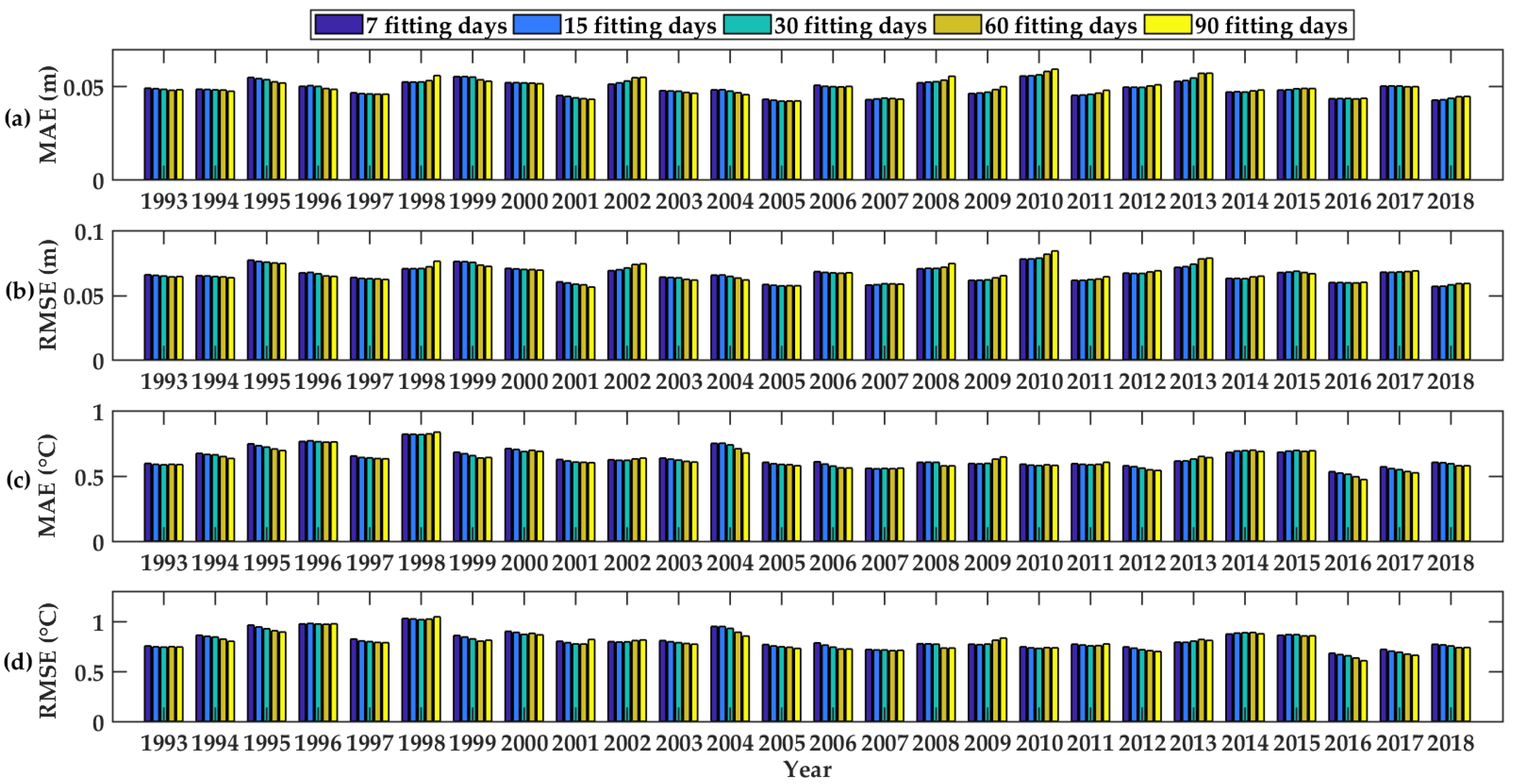
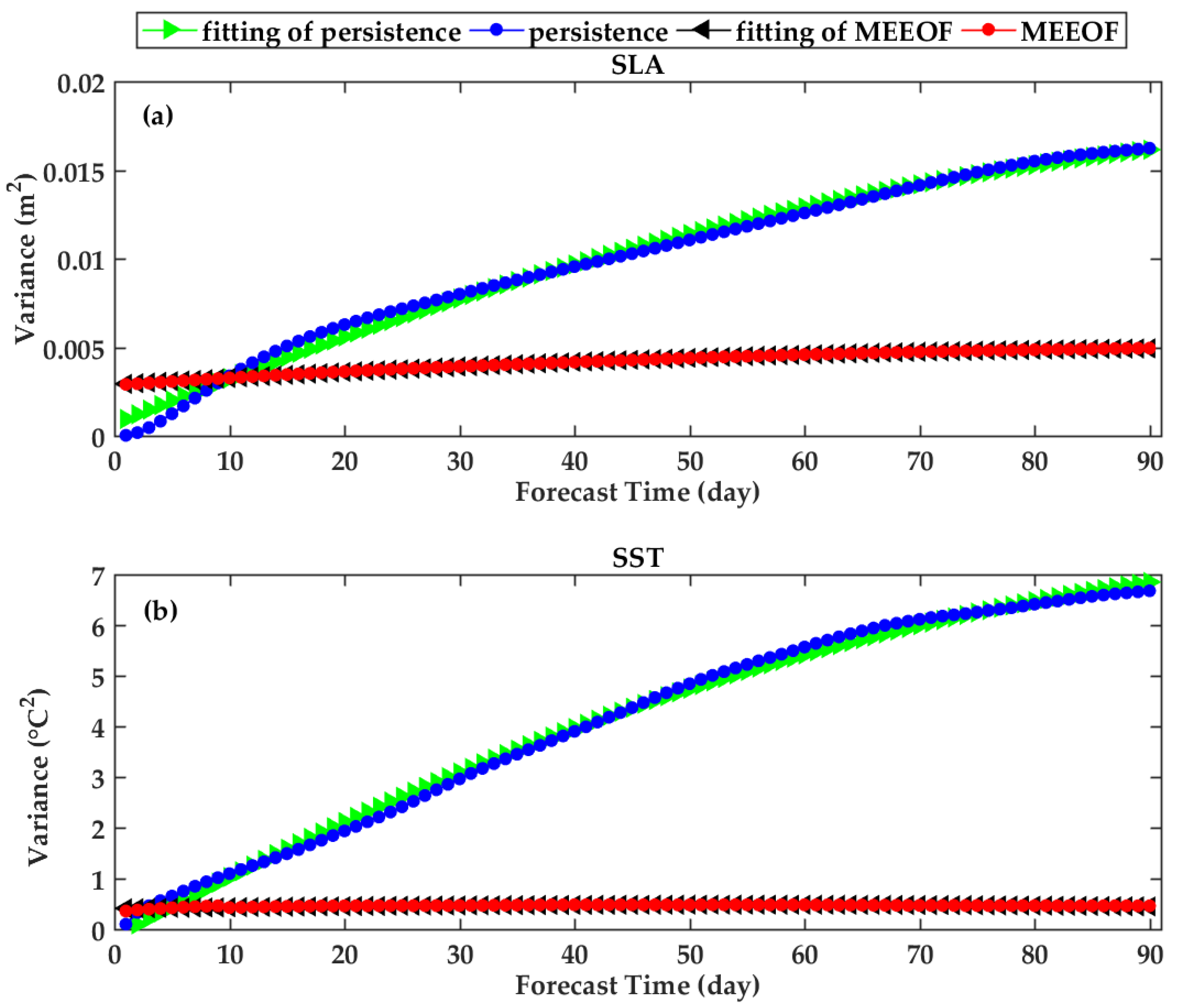
3.3. Fitting Performance and Parameters Determination

First, we design experiments to explore the prediction performance of this model for different fitting days. Here, we take the average forecast results of 1–60 days as the assessment standard to compare the forecasting results of different fitting days. In the experiments, 7, 15, 30, 60, and 90 fitting days are used, respectively. We use 24 MEEOFs here, the variance proportion of which is 100%. Figure 3 shows the MAE and RMSE results of the SLA and SST forecasts for different fitting days in the 26 experiments. It is easy to see from the figure that the overall forecast errors are relatively stable for both SLA and SST, indicating the reliability and stability of this prediction model. Notably, in this study, we use different sea surface variables for simultaneous modeling, and different variables have different evolutionary processes and different cycles. On this basis, the optimal fitting days need to be considered and selected comprehensively so that the simultaneous prediction performance of SLA and SST can be optimized. From Figure 3, we can see that different fitting days have different effects on the prediction performance of SLA and SST (Appendix B). When the fitting days are 60 days, the comprehensive prediction performance is the best; the MAEs of the temporal-basin averages of 1–60 days for SLA and SST are 0.0490 m and 0.628 °C, and the corresponding RMSEs for SLA and SST are 0.0664 m and 0.795 °C. The above statistical results are the average results over 26 trials.
Then, we investigate the performance of different forecast days. Based on the above results, we adopt 24 MEEOFs, and the number of fitting days is fixed at 60 days. The forecast performance for 7, 15, 30, 60, 90, and 120 days are compared in Figure 4, which shows the MAEs and RMSEs of SLA and SST at different forecast times. As can be seen from Figure 4, the changes in MAEs and RMSEs are relatively gentle as the forecast window is extended. The above conclusions hold for both SSHA and SST. We conclude that this prediction model has a potential advantage for intra-seasonal prediction. For the prediction of SLA, based on the MEEOF model, the spatial and temporal averaged MAEs from start time to 7, 15, 30, 60, 90, and 120 days are 0.0465 m, 0.0469 m, 0.0480 m, 0.0490 m, 0.0497 m, and 0.0502 m, respectively. At the same time, the corresponding RMSEs are 0.0629 m, 0.0636 m, 0.0649 m, 0.0664 m, 0.0676 m, and 0.0680 m, respectively. For the prediction of SST, the spatial-temporal average MAEs from start time to 7, 15, 30, 60, 90, and 120 days are 0.635 °C, 0.634 °C, 0.638 °C, 0.628 °C, 0.620 °C, and 0.615 °C, respectively. The corresponding RMSEs are 0.807 °C, 0.804 °C, 0.807 °C, 0.795 °C, 0.785 °C, and 0.780 °C, respectively. Considering the experimental results of these two sea surface variables, we chose 90 days for forecasting.

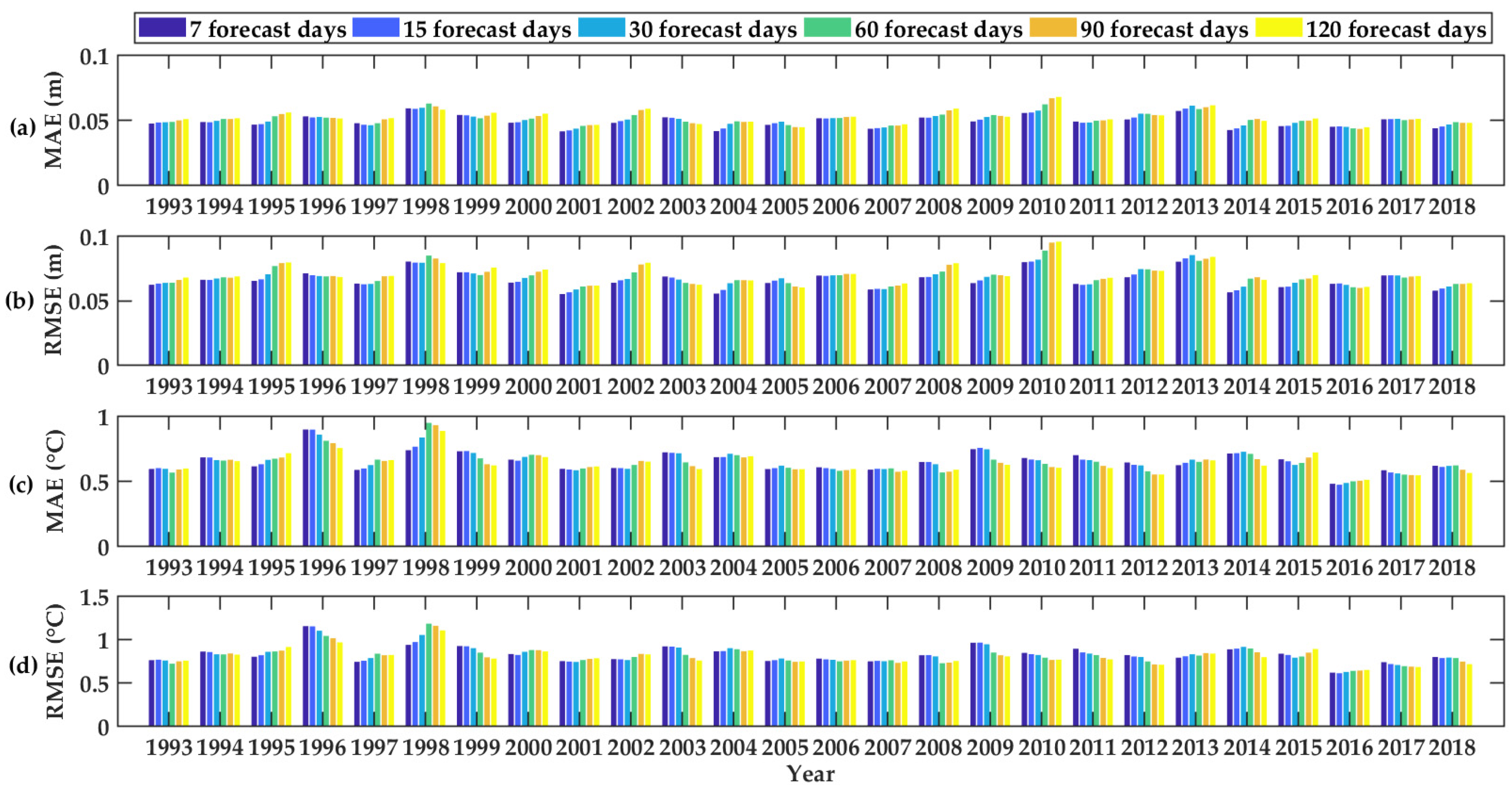
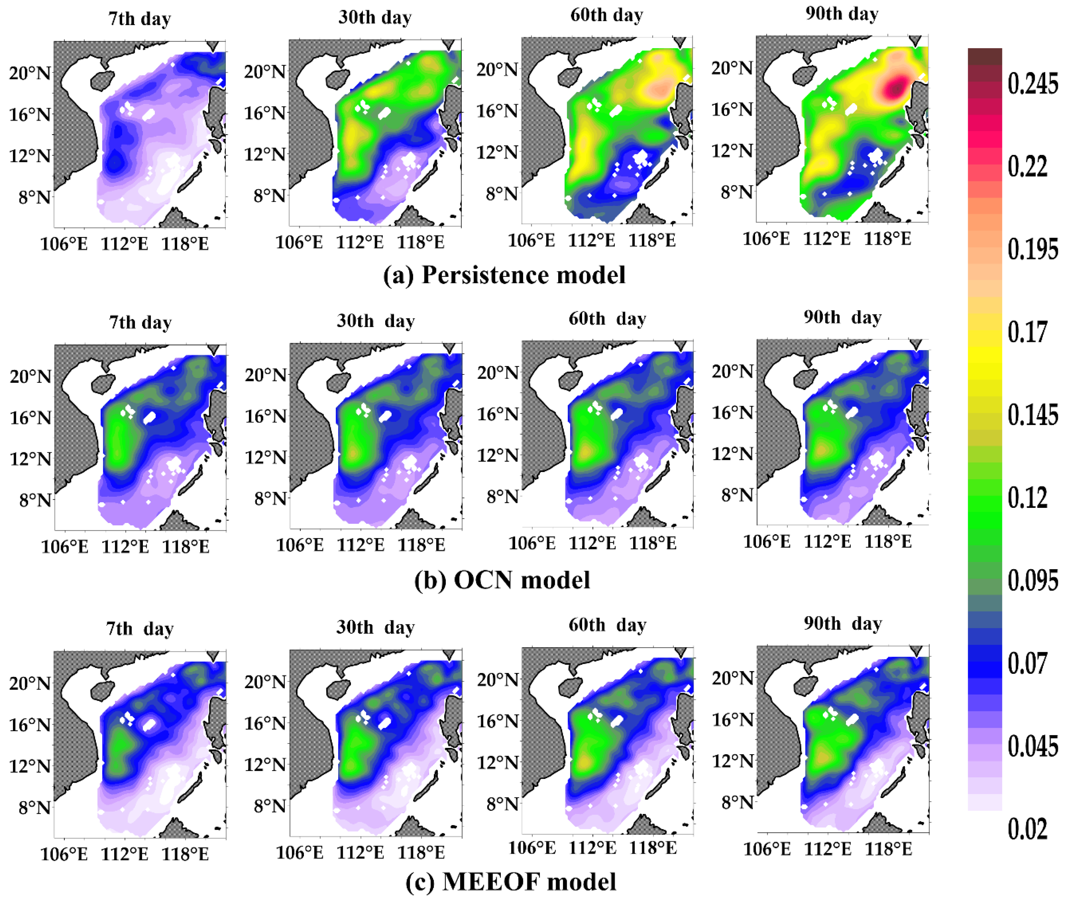
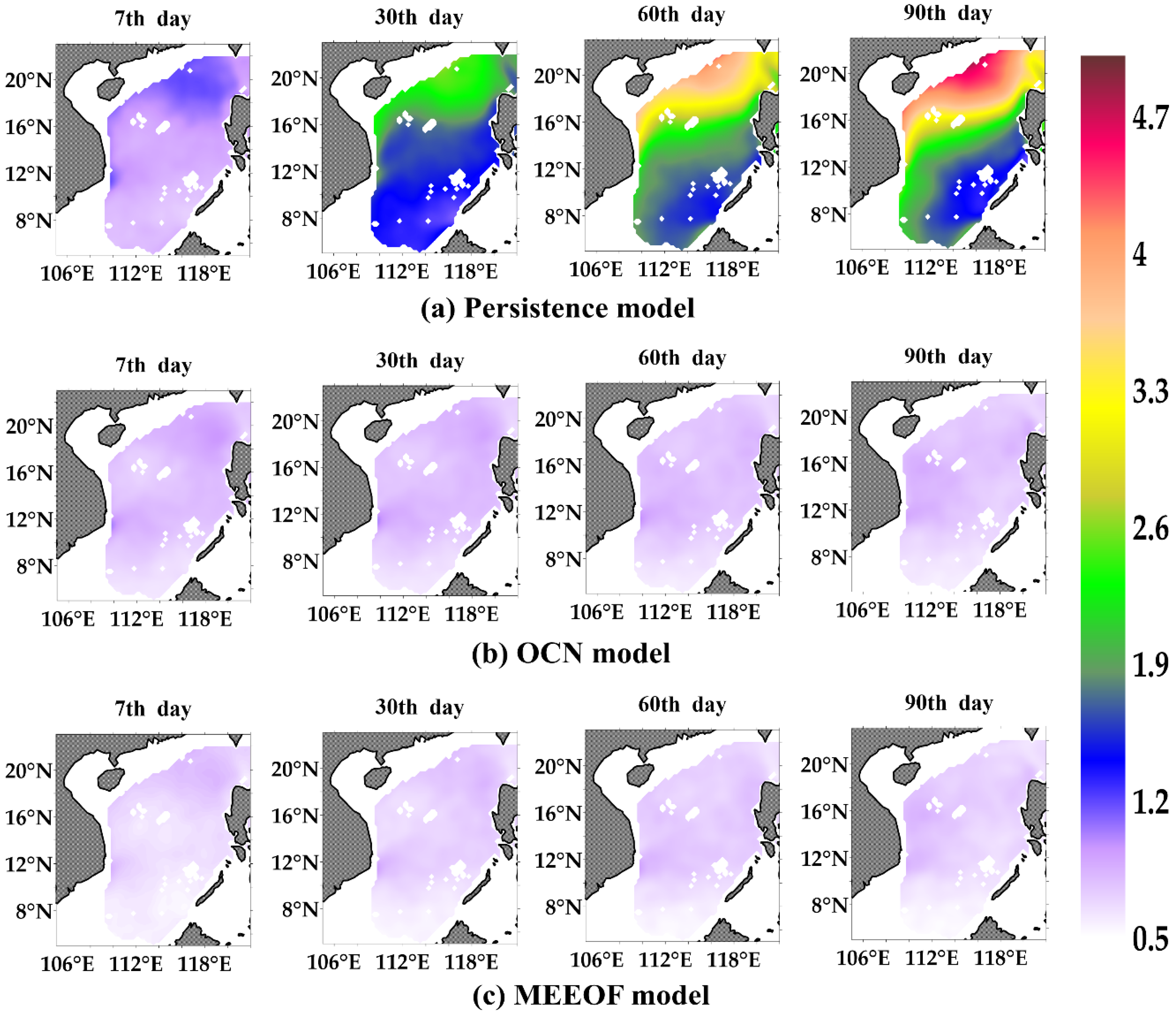
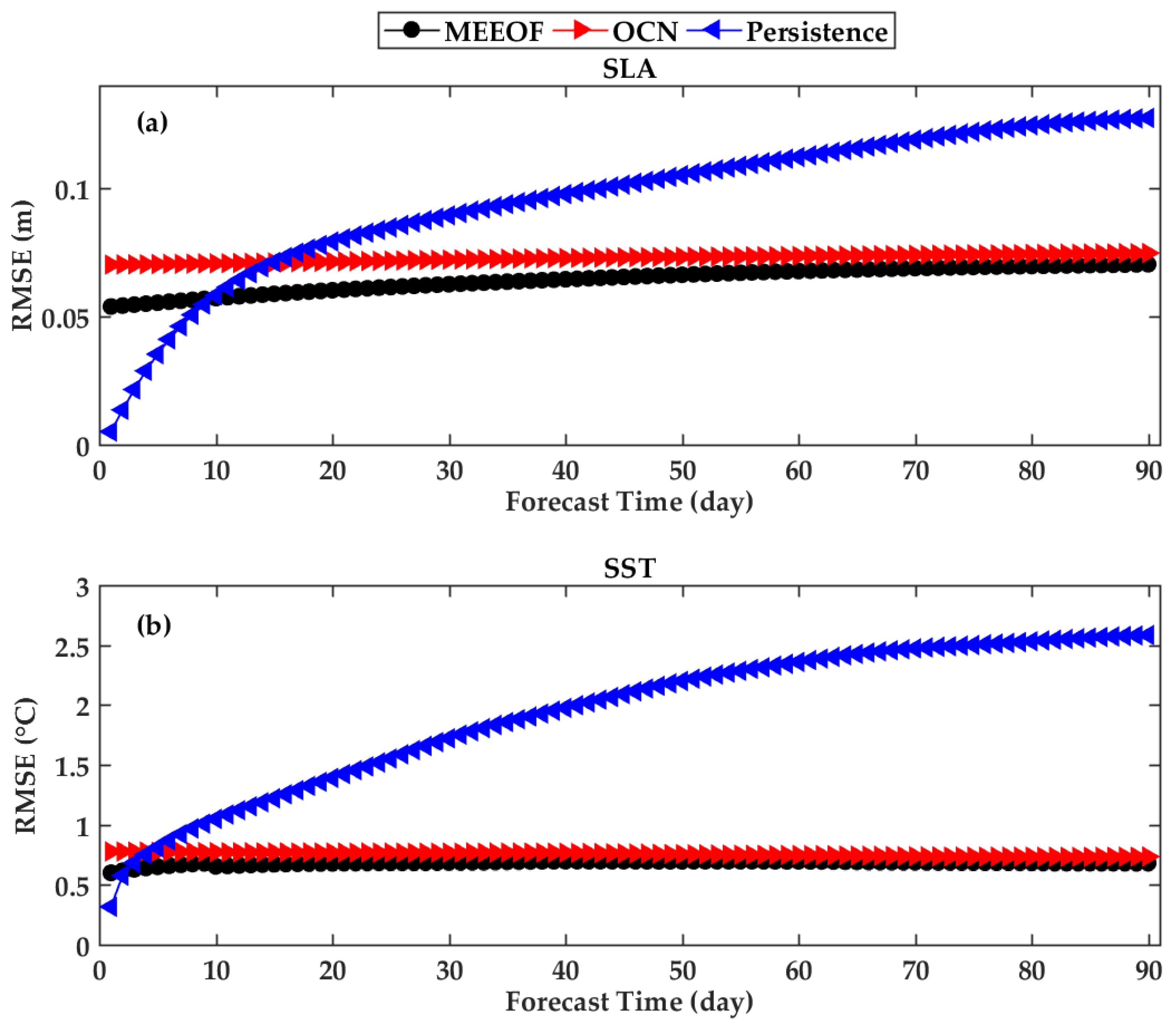
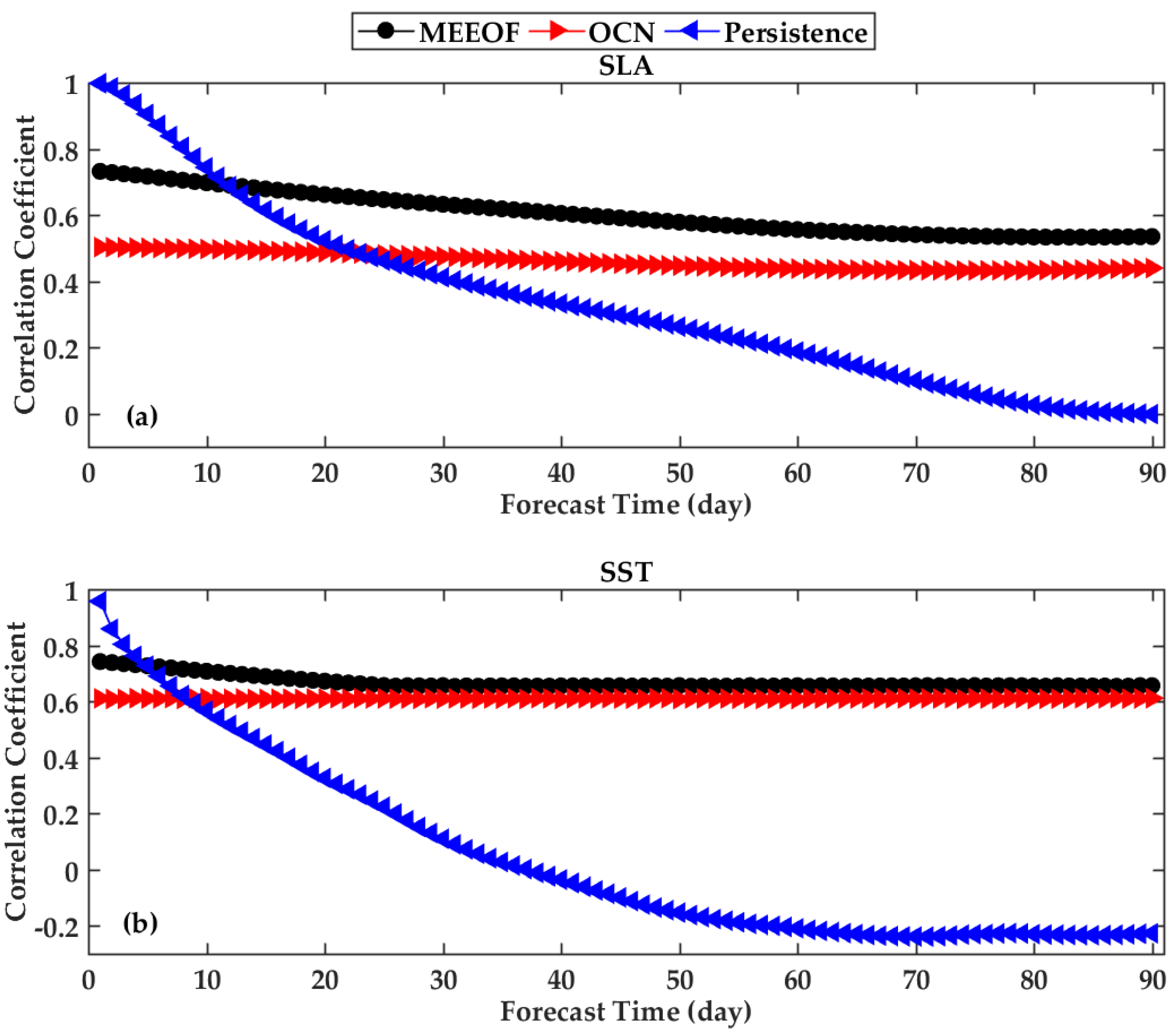
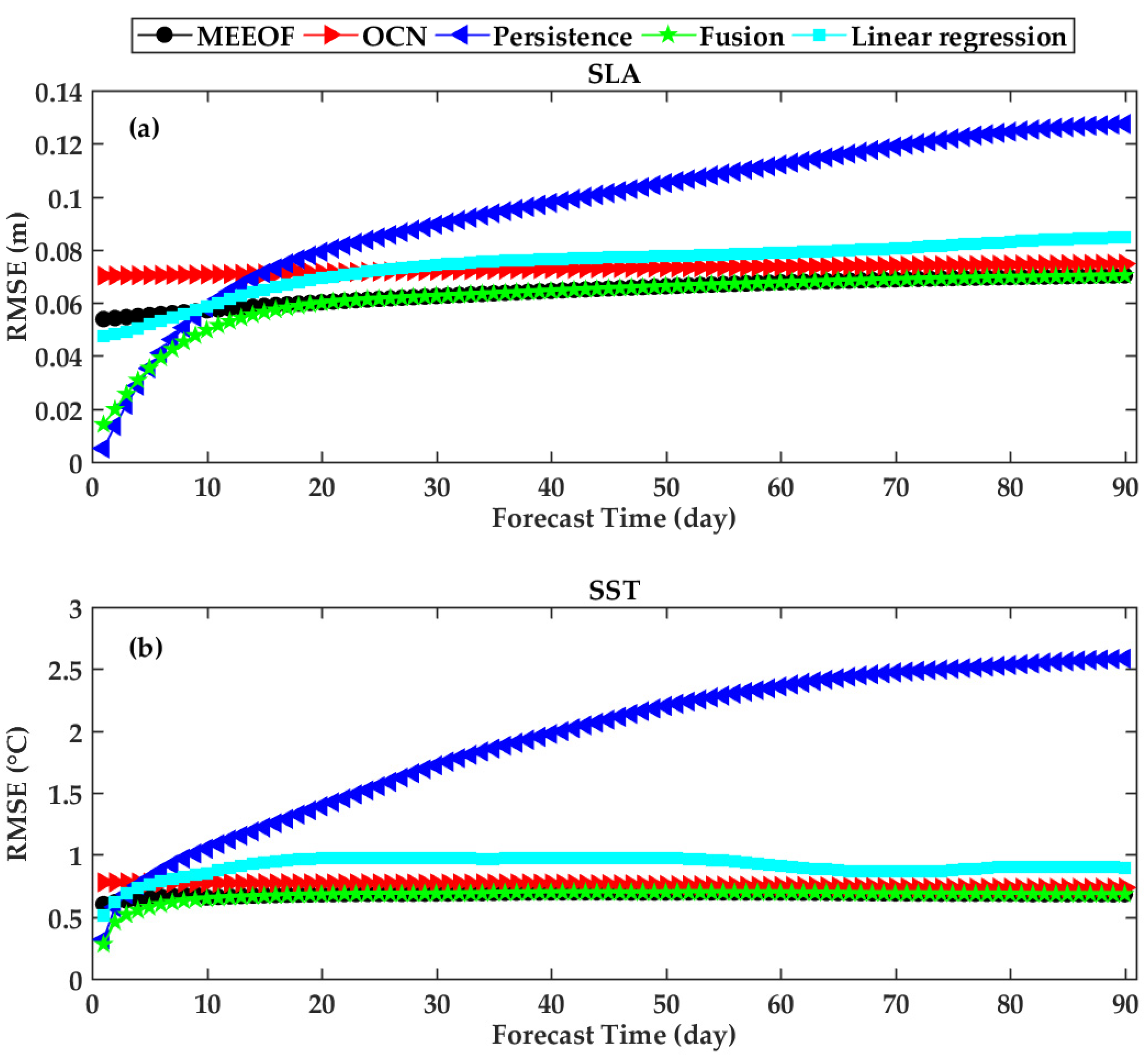
3.4. RMSE and CC Evaluation of Forecast Performance

Next, we show the model’s prediction performance. Based on the above model, we use 60 days for fitting and 90 days for prediction. Here, persistence prediction and the optimal climatic normal (OCN) method are compared with the MEEOF model. We use the above models to perform round-robin predictions to ensure the reliability of the experiments. Persistence prediction is a widely accepted reference for baseline comparisons in the atmospheric and oceanic sciences [40]. The basic idea is to assume that the ocean state at the initial moment will continue indefinitely throughout the entire forecast window. The OCN model is a common method for mid- and long-term ocean forecasting, and it uses the average of the previous k years as the subsequent forecast value [41]; here, the value of k is taken as 25. Suppose Z m , m = 1 , 2 , , 25 is a series of time data at yearly intervals, and the OCN prediction Z ¯ p is constructed as follows:
Z ¯ p = 1 25 j = 1 25 Z p j
where p = 26 here.
Figure 5, Figure 6, Figure 7 and Figure 8 show the basic statistics of the MEEOF model for the RMSEs and CCs of SLA and SST in the SCS. At the same time, as a comparison, the persistence and OCN prediction results for these two sea surface variables are also shown in these figures, by which the prediction capability of the MEEOF prediction model can be demonstrated.
The RMSEs of SLA forecasts validated at the 7th day, 30th day, 60th day, and 90th day are shown in Figure 5. Comparisons of the three models in Figure 5 show that the MEEOF prediction model outperforms the persistence and OCN forecasts over the 90-day forecast horizon. Although the persistence forecast has a small error at the beginning of the forecast window, its error grows rapidly as the forecast time increases, while the MEEOF model and OCN predictions remain largely stable throughout the entire forecast window. In particular, the error of the MEEOF model grows very slowly with the extension of the forecast window and is always smaller than that of the OCN model. This is also true for the SST forecasts (see also Figure 6). Thus, it can be concluded that the predictive capability of the MEEOF prediction model has an obvious advantage over persistence prediction in the mid- and long-term, and it outperforms the OCN prediction model throughout the entire forecast period.
As presented in Figure 5, these three models all show two areas with a large RMSE, one starting from the Luzon Strait, and the other area roughly located in the west-central part of the SCS, near Vietnam. It is well known that the Luzon Strait is the open boundary of the SCS, serving as a bridge for information exchange between the Northwest Pacific and the SCS. When the Kuroshio intrusion occurs, part of the Kuroshio water, with high temperature and high salinity, enters the SCS through the Luzon Strait and extends to the interior. Since the MEEOF model does not consider the influence of the boundary conditions, the error in this area cannot be well handled. Another area is located in the strong current zone, where ocean fronts are likely to be generated, resulting in a large variation in this area, which is obviously not well solved by the statistical model.
Figure 7 and Figure 8 show the overall performance of the MEEOF model in simultaneously forecasting SLA and SST. These figures show the basin-averaged temporal RMSE and CC, which are calculated from forecasts for every 90 days of the testing sets. From Figure 7, we see that the RMSEs of the MEEOF model for the SLA and SST forecasts are about 0.0703 m and 0.680 °C, respectively, when the prediction horizon is 90 days, while the RMSEs of the OCN predictions are about 0.0747 m and 0.734 °C. Next, to quantify the similarity between the predicted values and the real satellite remote sensing observations, the CCs are shown in Figure 8. It is easy to see that the CCs of persistence prediction decreases rapidly when the forecast time horizons range from 1 to 15 days, and the CC values of SLA and SST decrease from near 1 to near 0.6 and 0.45, respectively, indicating that this purely linear approach has good forecast performance only in the short term. However, both the MEEOF model and the OCN model take into account some fluctuations of the ocean, so the CC values of the MEEOF model and OCN model generally maintain a stable level. When the forecast time is 90 days, the CCs of the MEEOF for SLA and SST are approximately 0.54 and 0.66, but 0.44 and 0.61 for the OCN model, and the corresponding CCs of the persistence model are both less than 0.

4. Fusion Model

4.1. Description of the Fusion Model

From what has been discussed above, it is worth noting that the advantage of persistence forecasting is maintained in the short-term forecasts, while the benefit of the MEEOF forecasting is reflected in the mid- and long-term forecasts. Here, to ensure that the MEEOF model has good performance throughout the entire forecast window, we adopt a weighted average form of the persistence forecasts and the MEEOF forecasts in the final predictions. The final forecast can be expressed as follows:
X f ( k , t l ) = σ p e r s i s t e n c e 2 ( k , t l ) X M E E O F a ( k , t l ) + σ M E E O F 2 ( k , t l ) X p e r s i s t e n c e a ( k , t l ) σ p e r s i s t e n c e 2 ( k , t l ) + σ M E E O F 2 ( k , t l )
where X f ( k , t l ) , X M E E O F a ( k , t l ) , and X p e r s i s t e n c e a ( k , t l ) represent the prediction result of the fusion model, the MEEOF model, and the persistence model of the kth variable at time t l , respectively; σ p e r s i s t e n c e 2 ( k , t l ) and σ M E E O F 2 ( k , t l ) represent the variance of the persistence forecast and the MEEOF model, respectively.
Fitting the errors of the persistence model and the MEEOF model forecasts, the fitted variances of SLA and SST can be obtained as follows:
σ p e r s i s t e n c e 2 ( S L A , t l ) = 1.057 × 10 6 × ( t l ) 2 + 2.670 × 10 4 × ( t l ) + 0.0007
σ p e r s i s t e n c e 2 ( S S T , t l ) = 5.018 × 10 4 × ( t l ) 2 + 1.229 × 10 1 × ( t l ) 0.1468
σ M E E O F 2 ( S L A , t l ) = 1.851 × 10 7 × ( t l ) 2 + 3.935 × 10 5 × ( t l ) + 0.0029
σ M E E O F 2 ( S S T , t l ) = 2.656 × 10 5 × ( t l ) 2 + 0.0028 × ( t l ) + 0.4088
In addition, the previously noted error coefficients are calculated based on 26 trials. Figure 9 shows the error fitting results of the persistence and MEEOF predictions for SLA and SST.

4.2. Forecast Performance of the Fusion Model

Furthermore, we evaluate the prediction performance of the above fusion model, comparing it with the linear regression model [19], in addition to the traditional persistence forecasting and OCN model described above.
Here, the linear regression model is combined with the EOF analysis for predicting the sea surface multivariate. The specific process is: in each experiment, the multivariate dataset is decomposed by EOF analysis to obtain the orthogonal spatial modes (EOFs) and the corresponding PCs; then, the corresponding linear regression model is constructed for each PC series. Here, regression models are established as follows.
P i q = α 1 i q × p c 1 q + α 2 i q × p c 2 q + + α 60 i q × p c 60 q + c o n s i q ( i = 1 , , 90 ; q = 1 , , 29 )
where the predictand and predictor are denoted as P i q and p c i q , respectively, in which q represents the q th PC and i represents the lead time; α is the regression coefficient; c o n s i q is the constant term. Here, we keep the same experimental setup as in the MEEOF model, i.e., we use the information from the first 60 days to predict the states for the next 90 days. In this process, 4602 EOFs can be obtained, which is consistent with the number of grid points in one day for the two sea surface variables, but only 29 EOFs passed the significant test, so we use 29 PCs for modeling here.
The forecast performance of the fusion prediction model is further demonstrated in Figure 10 and Figure 11; the persistence prediction model, OCN results, MEEOF model, and linear regression model are also shown as comparisons. It is easy to see from the figures that the fusion model outperforms the persistence forecast within the short-term forecast. When the forecast window is continuously extended, the fusion model consistently outperforms the linear regression model and the OCN model.
From the above discussions, we understand that the forecast performance of the fusion model is more effective than the other comparative models. This is because traditional persistence forecasting assumes that the ocean variations occur in a purely linear manner over an infinite period of time, which is inconsistent with the real variations in the ocean environment, so the predictions are only valid for shorter periods of time; the linear regression method describes the processes of ocean change in terms of linear evolution over a finite period of time, which cannot be well described for the nonlinear signal; OCN model results generally represent a multiyear average, which describes the large-scale periodic signal of the ocean, and therefore, they are insufficient to describe the intra-seasonal variability of oceanic multiscale processes. However, the MEEOF prediction model effectively takes into account the fluctuations of the ocean, and when there is enough data, this model can effectively capture both the fluctuating and multiscale signals of the ocean. The fusion model combines the advantages of persistence forecasting in the short term and the advantages of MEEOF forecasting in the medium and long term, so it performs well on an intra-seasonal scale.

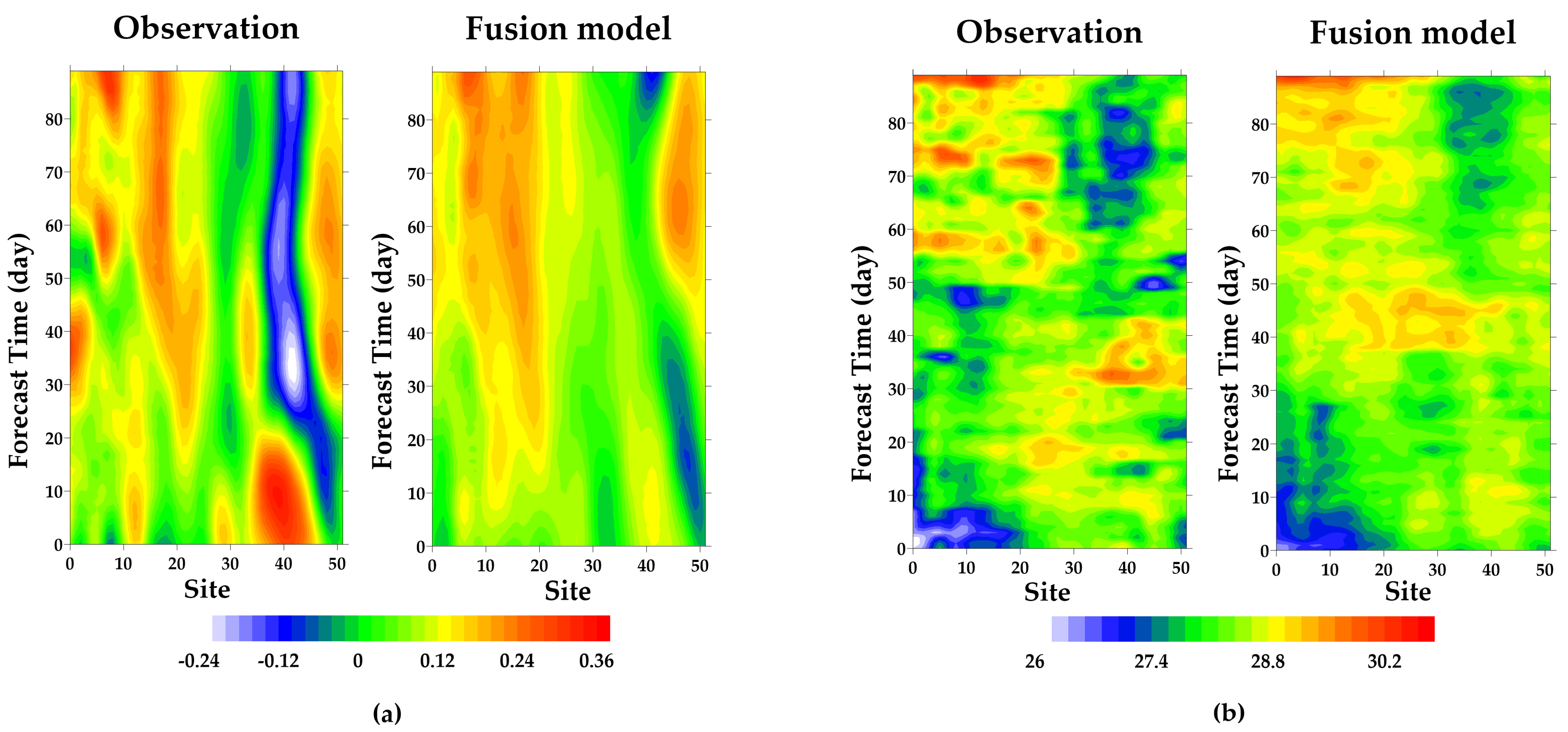
4.3. Forecast Example

Here, to further illustrate the effectiveness of the fusion model in forecasting the trends of ocean variables, we show the time-station map for SLA and SST. The red dots in Figure 12 represent the locations of the sampling sites—a total of 52 sampling points, extending from northeast to southwest in the SCS—as shown in this figure.
Figure 13 shows the temporal evolution of SLA and SST for the sampling sites, with a forecast window of 90 days, i.e., from 9 May 2018 to 6 August 2018; (a) and (b) indicate the temporal evolution of SLA and SST, respectively, where the horizontal coordinates indicate the sampling sites and the vertical coordinates indicate the forecast time. It can be seen from (a) that the prediction results of the fusion model are more consistent with the propagation trend of the waves in the true field, i.e., the propagation of the ocean waves is obvious. In addition, since the fusion model considers the coordinating relationship between SLA and SST, the coordination variations between these two sea surface variables can also be seen in Figure 13.

5. Discussion

In the SCS, which is a semi-enclosed basin, the internal dynamic processes play a much greater role than the external drivers for its intra-seasonal time scale evolutionary process, so the evolution of eddies and the propagation of ocean waves in the SCS follow their own evolutionary laws. In addition, the remote sensing data used in this study not only represent the current state of the ocean, but also imply its evolutionary process and the influence of other external driving forces. More importantly, unlike other linear methods, the MEEOF model in this study takes into account the evolution of oceanic fluctuations. Based on the above factors, we can see why the MEEOF model performs well in intra-seasonal scale forecasts.
In addition, through experiments using code performance, we find that this prediction model also has the advantages of simplicity and miniaturization. The time spent for the EEOF decomposition in this study is 483.330 s, which is much less than the running time of the numerical model forecasts. It is worth mentioning that in the practical operational prediction process, we only need to save the MEEOFs obtained from the above decomposition and project the observed data onto them, and the time for projection and prediction is much smaller than the time for the above decomposition process. Moreover, this forecasting model can be installed on any common workstation computer, with high portability. For operational forecasting, we can also directly use the error parameters of the persistence and MEEOF models in this study to construct the fusion model, since these errors are statistically significant. The above illustrates the advantages of this forecasting model for operational applications.
Finally, this prediction model has strong applicability. In addition to the sea surface prediction in this study, it can also be used in for predictions in the three-dimensional ocean, atmosphere, groundwater, etc.
However, there are still some limitations of this prediction model that need to be further discussed and addressed. First, it is worth noting that any data-driven model is directly related to the “amount” of the data, and the “amount” of the data we mentioned here consists of two parts: one is the number of variables and the other is the length of the dataset. Since we use satellite remote sensing data to construct the model in this study, the time length of the data and the number of variables are relatively small, and the system formed by them is not close enough, so the accuracy of the prediction results obtained by this model is not greatly improved. In addition, we do not consider the influence of the external drivers, such as atmosphere; thus, our model unable to make accurate forecasts under the abrupt oceanic conditions. Therefore, in subsequent studies, we will further improve the model by using long-time series ocean and atmosphere reanalysis data, considering the influence of external drivers such as the atmosphere of the ocean, and constructing a fusion model in an ocean-atmosphere coupled frame, so as to devise a more accurate set of spatiotemporal basis functions and improve the prediction accuracy.

6. Conclusions

In this study, we propose a simple model based on the traditional EEOF analysis to predict multiple sea surface variables simultaneously for intra-seasonal predictions, which is referred to as the MEEOF model. This model not only accounts for the spatial and temporal correlations across grid points, but also considers the dynamic balance between different sea surface variables, consistent with the real variations of the marine environment. Moreover, it embeds the temporal information into the spatial patterns, which effectively captures the spatial distribution and temporal evolution of the sea surface variables.
To evaluate the model’s forecast performance in the SCS, we conduct daily forecast experiments for SLA and SST. To ensure the reliability of the experimental results, we perform a round-robin experiment, i.e., the EEOF analysis is performed for any 25 years of data and then validated with another year of data. To better illustrate the superiority of the MEEOF model, persistence forecasting and the OCN model are used as comparisons, and RMSE and CC are used as the evaluation criteria; the comparison results show that the MEEOF model has a stable forecast performance in the forecast range of 15–90 days, and the rising trend of error is much slower. At the end of the forecast window, the RMSE and CC of the MEEOF model for SLA are 0.0703 m and 0.54, respectively; the RMSE and CC for SST are 0.680 °C and 0.66, respectively, which are better results than those using the persistence and OCN models.
Furthermore, to ensure that the MEEOF model has good forecasting performance in the short- to mid- and long-term, we adopt a weighted average form of persistence forecasts and the MEEOF forecasts for the final predictions, called the fusion model. It not only inherits the advantages of the MEEOF model in the mid- and long-term forecasts, but also rivals the persistence prediction model in the short-term forecasts. The fusion model also outperforms the linear regression model throughout the forecast period.

Author Contributions

Conceptualization, W.L.; data curation, Q.S.; formal analysis, Q.S. and W.L.; funding acquisition, Y.Z., G.H. (Guijun Han), W.L. and Q.S.; investigation, W.L. and G.H. (Guangchao Hou); resources, W.L. and Q.S.; software, G.H. (Guangchao Hou) and C.L.; supervision, S.L. and Y.G.; validation, H.L. and P.Q.; writing—original draft, Q.S.; writing—review and editing, Q.S. and W.L. All authors have read and agreed to the published version of the manuscript.

Funding

This research is cosponsored by grants from the National Natural Science Foundation of China (41876014) and the Open Project of the Tianjin Key Laboratory of Oceanic Meteorology (2020TKLOMYB04).

Data Availability Statement

SLA data is available in the Copernicus Marine Environment Monitoring Service (CMEMS) (http://marine.copernicus.eu) (accessed on 17 July 2021), and SST data is available in the NOAA (https://www.ncdc.noaa.gov/oisst) (accessed on 17 July 2021).

Acknowledgments

The authors would like to thank the following data and tool providers: Copernicus Marine Environment Monitoring Service (CMEMS) for providing SSHA data at http://marine.copernicus.eu (accessed on 17 July 2021), and NOAA for providing OISST data, the website is https://www.ncdc.noaa.gov/oisst (accessed on 17 July 2021).

Conflicts of Interest

The authors declare no conflict of interest.

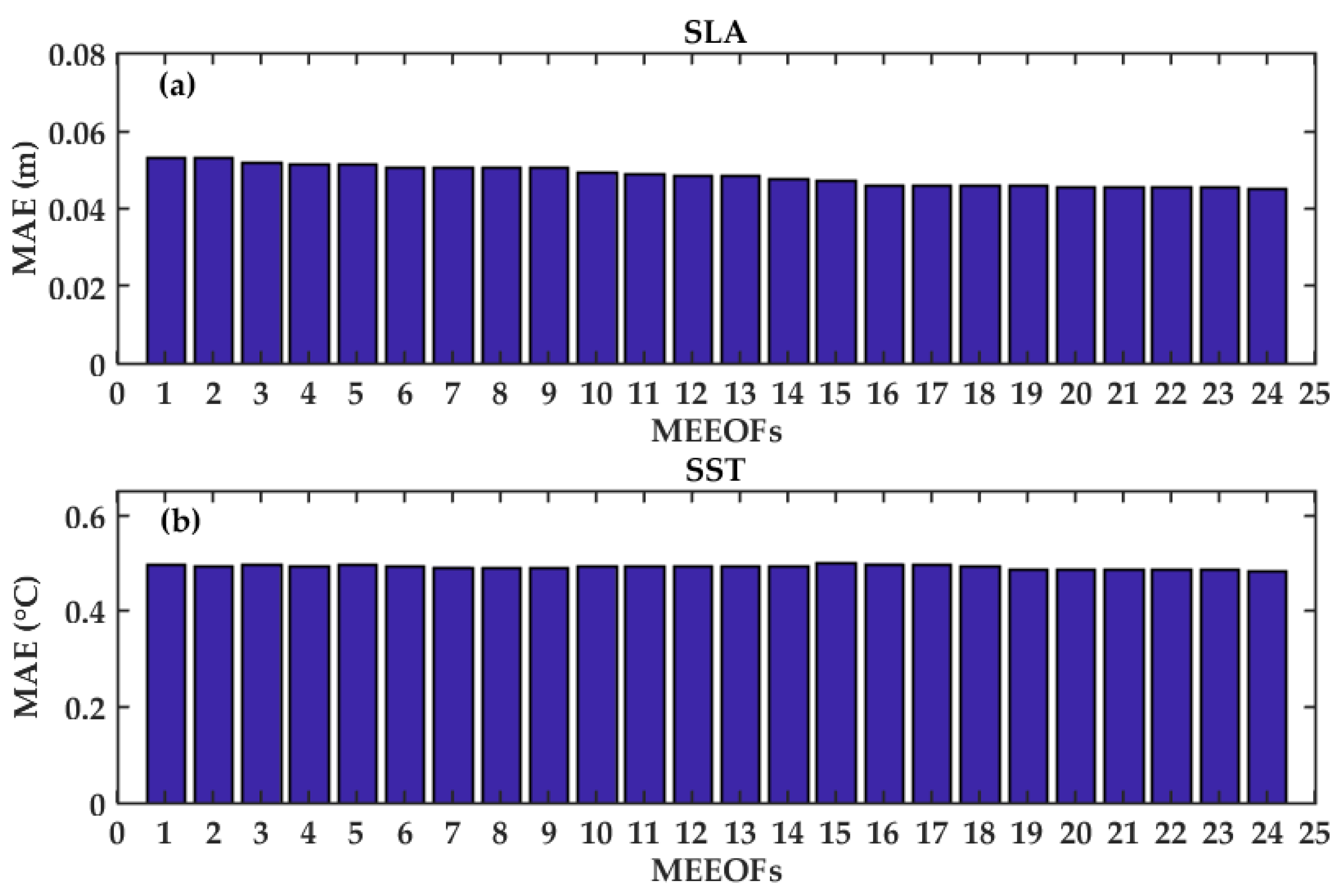
Appendix A. Choice of MEEOFs

Here, we design experiments to determine the optimal number of MEEOFs to achieve the best fitting performance to the observational data. Therefore, we conduct the fitting experiments on the independent testing set. Taking the 90-day fitting as an example, different amounts of MEEOFs are used to fit the data on the independent testing set. Figure A1 in Appendix A shows the statistical results of the fitting mean absolute error of the SSHA and SST, respectively, both of which are the average results of 90 days. As can be seen in Figure A1, 24 MEEOFs are optimal for fitting (the number of MEEOFs that minimizes the error in the cross-validation), and the variance proportion of these 24 MEEOFs is 100%. The above conclusion is held for each experiment. When the number of MEEOFs is 24, the fitting mean absolute errors of SSHA and SST within 90 days minimize the expected error to 0.0451 m and 0.484 °C, respectively.
In fact, the number of MEEOFs has a significant influence on both the fitting performance and the prediction performance. As the number of MEEOFs increases, the total proportion of spatiotemporal modes increases, the interpretable variance becomes larger, and the phase space formed by these MEEOFs becomes more complete. In other words, the more MEEOFs we use, the better the interpretation of the spatial characteristics and the temporal evolution process of the sea surface variables. Notably, in each experiment, all of the 24 MEEOFs passed the significance test [42].
Figure A1. The mean absolute error within 90 days, obtained by the cross-validation for fitting experiment—(a) SLA; (b) SST.
Remotesensing 14 01162 g0a1

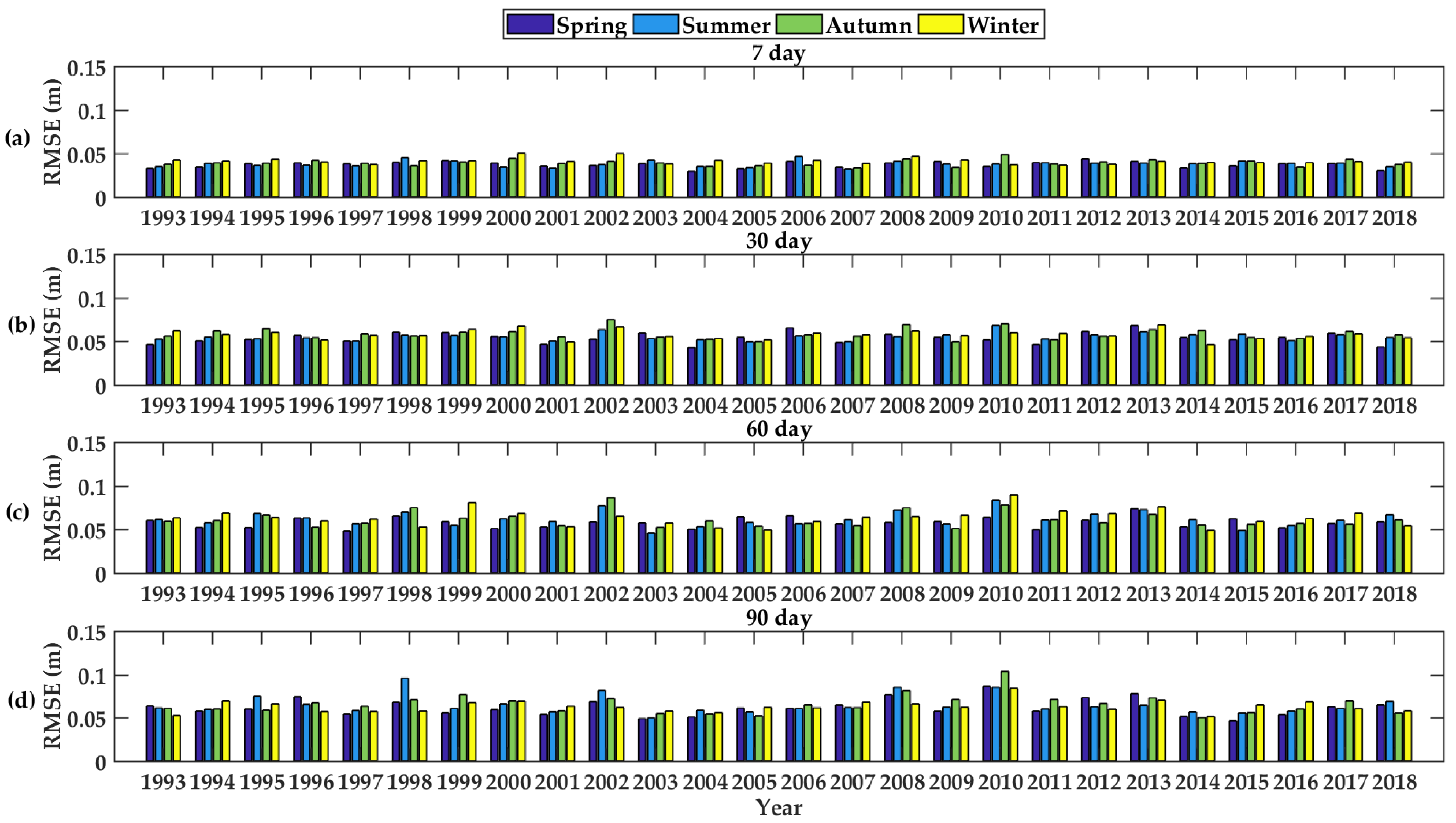
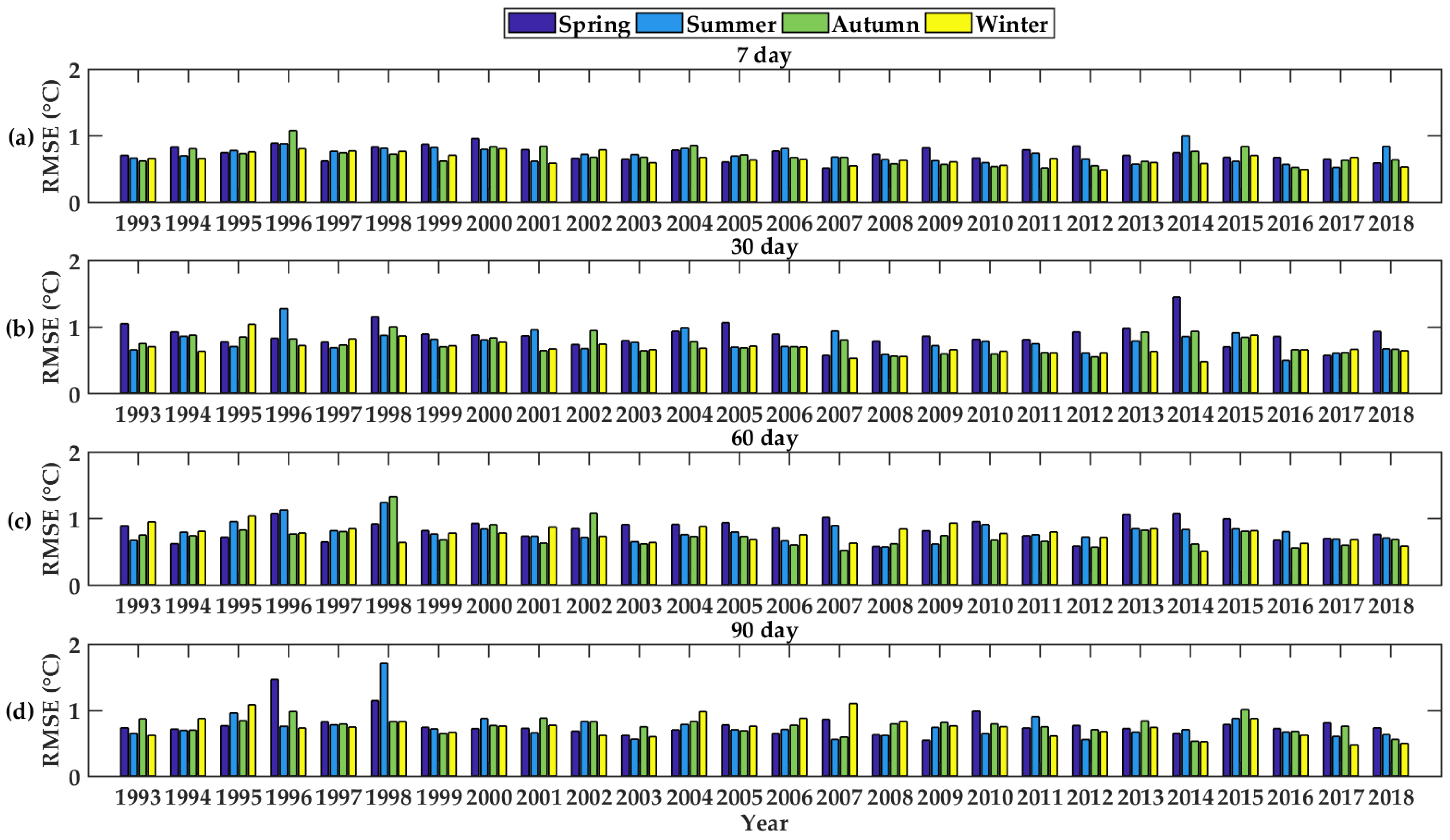
Appendix B. Seasonal Performance

Here, we conduct experiments to compare the prediction performance of the fusion model in different seasons. Four different seasons are classified as follows: spring (March, April, and May), summer (June, July, and August), autumn (September, October, and November), and winter (December, January, and February). The RMSE of SLA and SST for different seasons and different forecast days are shown in Figure A2 and Figure A3.
For SLA forecasts, when the forecast time is 7 days, the forecast RMSEs of the fusion model in spring, summer, autumn, and winter are 0.0372 m, 0.0381 m, 0.0392 m, and 0.0412 m, respectively; when the forecast time is 30 days, the corresponding forecast RMSEs are 0.0539 m, 0.0552 m, 0.0584 m, and 0.0576 m, respectively; when the forecast time is 60 days, the corresponding forecast RMSEs are 0.0579 m, 0.0619 m, 0.0612 m, and 0.0634 m, respectively; and when the forecast time is 90 days, the corresponding forecast RMSEs are 0.0621 m, 0.0650 m, 0.0656 m, and 0.0630 m, respectively.
Then, for the forecasts of SST, when the forecast time is 7 days, the forecast RMSEs of the fusion model in spring, summer, autumn, and winter are 0.730 °C, 0.712 °C, 0.689 °C, and 0.646 °C, respectively; when the forecast time is 30 days, the corresponding forecast RMSEs are 0.874 °C, 0.772 °C, 0.739 °C, and 0.687 °C, respectively; when the forecast time is 60 days, the corresponding forecast RMSEs are 0.833 °C, 0.792 °C, 0.729 °C, and 0.762 °C, respectively; when the forecast time is 90 days, the corresponding forecast RMSEs are 0.773 °C, 0.748 °C, 0.764 ℃, and 0.740 °C, respectively.
All the above results are the average statistics of the 26 experiments.
Figure A2. The forecast results of SLA for different seasons—(a) for the prediction time of 7 day, and (bd) for 30 day, 60 day and 90 day, respectively.
Remotesensing 14 01162 g0a2
Figure A3. Same as Figure A2, but for SST—(a) for the prediction time of 7 day, and (bd) for 30 day, 60 day and 90 day, respectively.
Remotesensing 14 01162 g0a3

References

  1. Schiller, A.; Brassington, G.B. Operational Oceanography in the 21st Century; Springer Science & Business Media: Berlin/Heidelberg, Germany, 2011. [Google Scholar]
  2. Francis, P.A.; Vinayachandran, P.N.; Shenoi, S.S.C. The Indian Ocean Forecast System. Curr. Sci. 2013, 104, 1354–1368. [Google Scholar]
  3. Wang, G. Mesoscale eddies in the South China Sea observed with altimeter data. Geophys. Res. Lett. 2003, 30, 2121. [Google Scholar] [CrossRef] [Green Version]
  4. Pei, Y.; Zhang, R.-H.; Zhang, X.; Jiang, L.; Wei, Y. Variability of sea surface height in the South China Sea and its relationship to Pacific oscillations. Acta Oceanol. Sin. 2015, 34, 80–92. [Google Scholar] [CrossRef]
  5. Jianyu, H.; Kawamura, H.; Huasheng, H.; Kobash, F.; Dongxiao, W. 3~6 Months Variation of Sea Surface Height in the South China Sea and Its Adjacent Ocean. J. Oceanogr. 2001, 57, 69–78. [Google Scholar]
  6. Xiu, P.; Chai, F.; Shi, L.; Xue, H.; Chao, Y. A census of eddy activities in the South China Sea during 1993–2007. J. Geophys. Res. 2010, 115. [Google Scholar] [CrossRef] [Green Version]
  7. Patil, K.; Deo, M.C.; Ravichandran, M. Prediction of Sea Surface Temperature by Combining Numerical and Neural Techniques. J. Atmos. Ocean. Technol. 2016, 33, 1715–1726. [Google Scholar] [CrossRef]
  8. Barron, C.N.; Birol Kara, A.; Hurlburt, H.E.; Rowley, C.; Smedstad, L.F. Sea Surface Height Predictions from the Global Navy Coastal Ocean Model during 1998–2001. J. Atmos. Ocean. Technol. 2004, 21, 1876–1893. [Google Scholar] [CrossRef] [Green Version]
  9. Rowley, C.; Banon, C.; Smedstad, L.; Rhodes, R. Real-time ocean data assimilation and prediction with global NCOM. In Proceedings of the OCEANS ‘02 MTS/IEEE, Biloxi, MI, USA, 29–31 October 2002; pp. 775–780. [Google Scholar]
  10. Chassignet, E.; Hurlburt, H.; Metzger, E.J.; Smedstad, O.; Cummings, J.; Halliwell, G.; Bleck, R.; Baraille, R.; Wallcraft, A.; Lozano, C.; et al. US GODAE: Global Ocean Prediction with the HYbrid Coordinate Ocean Model (HYCOM). Oceanography 2009, 22, 64–75. [Google Scholar] [CrossRef]
  11. Powell, B.S.; Moore, A.M.; Arango, H.G.; Di Lorenzo, E.; Milliff, R.F.; Leben, R.R. Near real-time ocean circulation assimilation and prediction in the Intra-Americas Sea with ROMS. Dyn. Atmos. Ocean. 2009, 48, 46–68. [Google Scholar] [CrossRef]
  12. Noori, R.; Abbasi, M.R.; Adamowski, J.F.; Dehghani, M. A simple mathematical model to predict sea surface temperature over the northwest Indian Ocean. Estuar. Coast. Shelf Sci. 2017, 197, 236–243. [Google Scholar] [CrossRef] [Green Version]
  13. Cummings, J.A. Operational multivariate ocean data assimilation. Q. J. R. Meteorol. Soc. 2005, 131, 3583–3604. [Google Scholar] [CrossRef] [Green Version]
  14. Carman, J.C.; Eleuterio, D.P.; Gallaudet, T.C.; Geernaert, G.L.; Harr, P.A.; Kaye, J.A.; McCarren, D.H.; McLean, C.N.; Sandgathe, S.A.; Toepfer, F.; et al. The National Earth System Prediction Capability: Coordinating the Giant. Bull. Am. Meteorol. Soc. 2017, 98, 239–252. [Google Scholar] [CrossRef] [Green Version]
  15. Drévillon, M.; Bourdallé-Badie, R.; Derval, C.; Lellouche, J.M.; Rémy, E.; Tranchant, B.; Benkiran, M.; Greiner, E.; Guinehut, S.; Verbrugge, N.; et al. The GODAE/Mercator-Ocean global ocean forecasting system: Results, applications and prospects. J. Oper. Oceanogr. 2014, 1, 51–57. [Google Scholar] [CrossRef]
  16. Miyazawa, Y. Ensemble forecast of the Kuroshio meandering. J. Geophys. Res. 2005, 110, C10026. [Google Scholar] [CrossRef] [Green Version]
  17. Jifan, C. Predictability Of The Atmosphere. Adv. Atmos. Sci. 1988, 6, 335–346. [Google Scholar] [CrossRef]
  18. Patil, K.; Deo, M.C. Basin-Scale Prediction of Sea Surface Temperature with Artificial Neural Networks. J. Atmos. Ocean. Technol. 2018, 35, 1441–1455. [Google Scholar] [CrossRef]
  19. Kug, J.; Kang, I.; Lee, J.; Jhun, J. A statistical approach to Indian Ocean sea surface temperature prediction using a dynamical ENSO prediction. Geophys. Res. Lett. 2004, 31, 112–124. [Google Scholar] [CrossRef]
  20. Tang, B.; Hsieh, W.W.; Monahan, A.H.; Tangang, F.T. Skill Comparisons between Neural Networks and Canonical Correlation Analysis in Predicting the Equatorial Pacific Sea Surface Temperatures. J. Clim. 2000, 13, 287–293. [Google Scholar] [CrossRef] [Green Version]
  21. Xue, Y.; Leetmaa, A. Forecasts of tropical Pacific SST and sea level using a Markov model. Geophys. Res. Lett. 2000, 27, 2701–2704. [Google Scholar] [CrossRef] [Green Version]
  22. Wei, L.; Guan, L.; Qu, L. Prediction of Sea Surface Temperature in the South China Sea by Artificial Neural Networks. IEEE Geosci. Remote Sens. Lett. 2019, 17, 558–562. [Google Scholar] [CrossRef]
  23. Wei, L.; Guan, L.; Qu, L.; Guo, D. Prediction of Sea Surface Temperature in the China Seas Based on Long Short-Term Memory Neural Networks. Remote Sens. 2020, 12, 2697. [Google Scholar] [CrossRef]
  24. Imani, M.; You, R.-J.; Kuo, C.-Y. Analysis and prediction of Caspian Sea level pattern anomalies observed by satellite altimetry using autoregressive integrated moving average models. Arab. J. Geosci. 2013, 7, 3339–3348. [Google Scholar] [CrossRef]
  25. Patil, K.; Deo, M.C. Prediction of daily sea surface temperature using efficient neural networks. Ocean Dyn. 2017, 67, 357–368. [Google Scholar] [CrossRef]
  26. Shaw, P.-T. The seasonal variation of the intrusion of the Philippine sea water into the South China Sea. J. Geophys. Res. Ocean. 1991, 96, 821–827. [Google Scholar] [CrossRef]
  27. Hu, W.; Wu, R.; Liu, Y. Relation of the South China Sea Precipitation Variability to Tropical Indo-Pacific SST Anomalies during Spring-to-Summer Transition. J. Clim. 2014, 27, 5451–5467. [Google Scholar] [CrossRef]
  28. NOAA. Optimum Interpolation Sea Surface Temperature (OISST). Available online: https://www.ncdc.noaa.gov/oisst (accessed on 17 July 2021).
  29. Chu, P.C.; Ivanov, L.M.; Korzhova, T.P.; Margolina, T.M.; Melnichenko, O.V. Analysis of Sparse and Noisy Ocean Current Data Using Flow Decomposition. Part I: Theory. J. Atmos. Ocean. Technol. 2003, 20, 478–491. [Google Scholar] [CrossRef]
  30. Yuan, D.; Han, W.; Hu, D. Surface Kuroshio path in the Luzon Strait area derived from satellite remote sensing data. J. Geophys. Res. 2006, 111, 1–16. [Google Scholar] [CrossRef] [Green Version]
  31. North, G.R. Empirical Orthogonal Functions and Normal Modes. J. Atmos. Sci. 1983, 41, 879–887. [Google Scholar] [CrossRef] [Green Version]
  32. Lorenz, E.N. Empirical orthogonal functions and statistical weather prediction. Dept. Meteorol. Mass. Inst. Technol. Stat. Forecast. Proj. Rep 1956, 1, 1–49. [Google Scholar] [CrossRef]
  33. Chavez, F.; Messié, M. Global Modes of Sea Surface Temperature Variability in Relation to Regional Climate Indices. J. Clim. 2011, 24, 4314–4331. [Google Scholar] [CrossRef]
  34. Deser, C.; Alexander, M.A.; Xie, S.P.; Phillips, A.S. Sea surface temperature variability: Patterns and mechanisms. Ann. Rev. Mar. Sci. 2010, 2, 115–143. [Google Scholar] [CrossRef] [Green Version]
  35. Zhao, Y.; Feng, G.; Zheng, Z.; Zhang, D.; Jia, Z. Evolution of tropical interannual sea surface temperature variability and its connection with boreal summer atmospheric circulations. Int. J. Climatol. 2019, 40, 2702–2716. [Google Scholar] [CrossRef]
  36. Lau, K.H.; Lau, N.C. Observed structure and propagation characteristics of tropical summertime synoptic scale disturbances. Mon. Weather Rev. 1990, 118, 1888–1913. [Google Scholar] [CrossRef]
  37. Weare, B.C.; Nasstrom, J.S. Examples of extended empirical orthogonal function analyses. Mon. Weather Rev. 1982, 110, 481–485. [Google Scholar] [CrossRef]
  38. Mares, C.; Mares, I. Improvement of Long-Range Forecasting by EEOF Extrapolation Using an AR-MEM Model. Weather Forecast. 2003, 18, 311–324. [Google Scholar] [CrossRef]
  39. Fox, D.N.; Teague, W.J.; Barron, C.N. The Modular Ocean Data Assimilation System. J. Atmos. Ocean. Technol. 2000, 19, 240–252. [Google Scholar] [CrossRef]
  40. Li, J.; Wang, G.; Xue, H.; Wang, H. A simple predictive model for the eddy propagation trajectory in the northern South China Sea. Ocean Sci. 2019, 15, 401–412. [Google Scholar] [CrossRef] [Green Version]
  41. Huang, J.; Barnston, A.G. Long-Lead Seasonal Temperature Prediction Using Optimal Climate Normals. J. Clim. 1996, 9, 809–817. [Google Scholar] [CrossRef]
  42. North, G.R.; Bell, T.L.; Cahalan, R.F.; Moeng, F.J. Sampling Errors in the Estimation of Empirical Orthogonal Functions. Mon. Weather Rev. 1982, 110, 699–706. [Google Scholar] [CrossRef]
Figure 1. Study area—the SCS, with the Sulu Sea and shallower sea excluded.
Remotesensing 14 01162 g001
Figure 2. Flowchart of the MEEOF prediction model.
Remotesensing 14 01162 g002
Figure 3. Spatial and temporal average forecast results for different fitting days—(a,b) for SLA; (c,d) for SST.
Remotesensing 14 01162 g003
Figure 4. Spatial and temporal average forecast results for different forecast days—(a,b) for SLA; (c,d) for SST.
Remotesensing 14 01162 g004
Figure 5. Spatial maps of the prediction RMSE (m) of SLA at the 7th day, 30th day, 60th day, and 90th day—(a) for the persistence model, (b) for the OCN model, and (c) for the MEEOF model.
Remotesensing 14 01162 g005
Figure 6. The same spatial maps as in Figure 5, but for SST (°C)—(a) for the persistence model, (b) for the OCN model, and (c) for the MEEOF model.
Remotesensing 14 01162 g006
Figure 7. The basin average RMSEs of the MEEOF prediction model, persistence forecasting, and OCN model—(a) SLA; (b) SST.
Remotesensing 14 01162 g007
Figure 8. The same as Figure 7, but for the CCs—(a) SLA; (b) SST.
Remotesensing 14 01162 g008
Figure 9. The error fitting results of the persistence and MEEOF predictions—(a) for SLA; (b) for SST.
Remotesensing 14 01162 g009
Figure 10. Comparison of forecast RMSEs from the fusion model using persistence prediction, the OCN model, the MEEOF model, and the linear regression model—(a) SLA; (b) SST.
Remotesensing 14 01162 g010
Figure 11. The same as Figure 10, but for the CCs—(a) SLA; (b) SST.
Remotesensing 14 01162 g011
Figure 12. The position distribution of the selected section.
Remotesensing 14 01162 g012
Figure 13. The time-station map of the observation field and forecast field by fusion model from 9 May 2018 to 6 August 2018—(a) represents SLA and (b) represents SST.
Remotesensing 14 01162 g013
Table 1. Running time(s) for EEOF decomposition.
The Number of SubsamplesmnRunning Time(s)
20-year1,679,73020331.860
21-year1,679,73021358.150
22-year1,679,73022382.580
23-year1,679,73023411.270
24-year1,679,73024445.730
25-year1,679,73025483.330
Publisher’s Note: MDPI stays neutral with regard to jurisdictional claims in published maps and institutional affiliations.

