
Harmonization of Multi-Mission High-Resolution Time Series: Application to BELAIR


Abstract
:1. Introduction
2. Materials
2.1. Satellite Missions Considered in the Study
2.1.1. PROBA-V
2.1.2. DEIMOS-1
2.1.3. Sentinel-2
2.1.4. Landsat-8
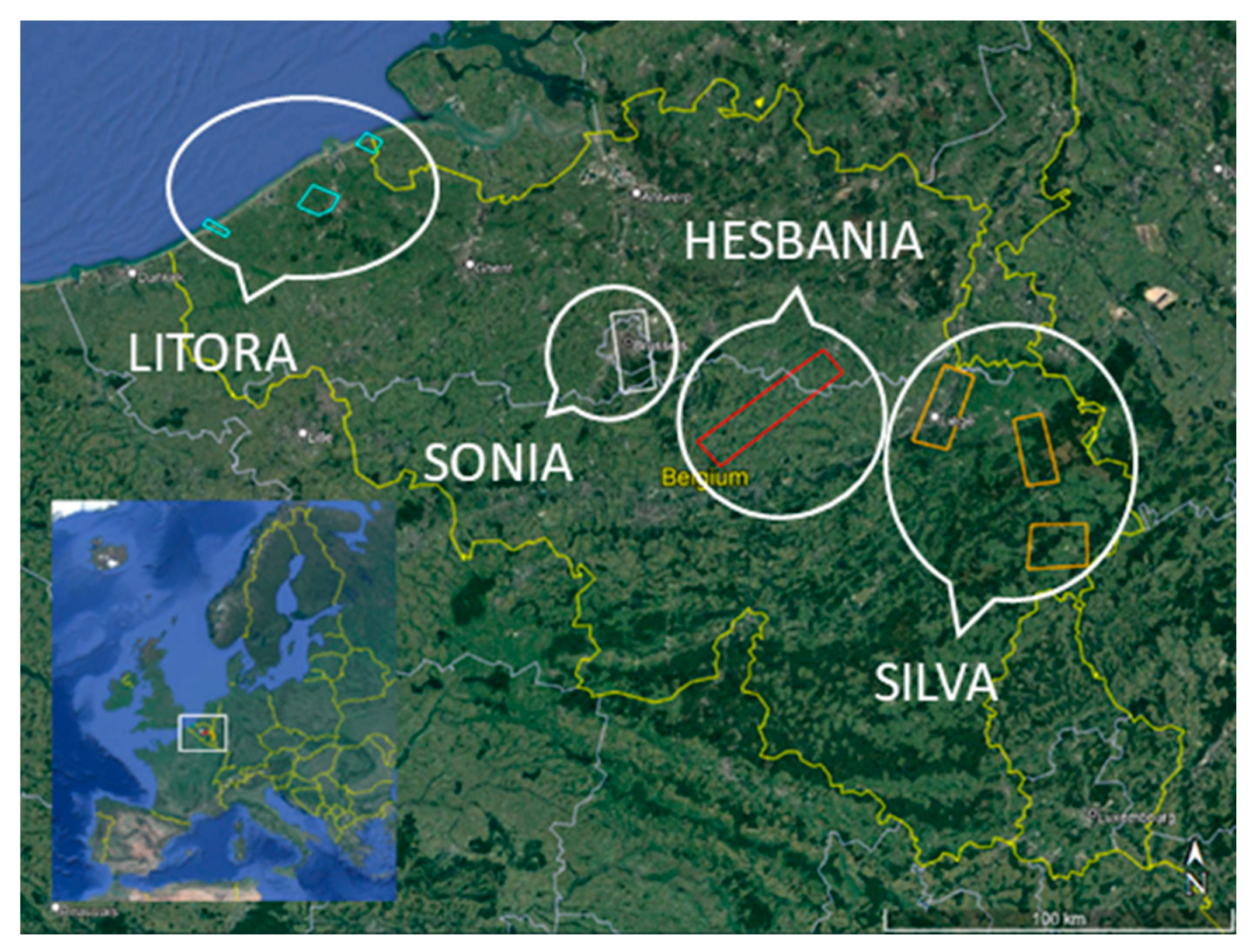
2.2. Case Sites
2.2.1. HESBANIA Agricultural Case Study
2.2.2. SONIA Urban Case Study
3. Methods
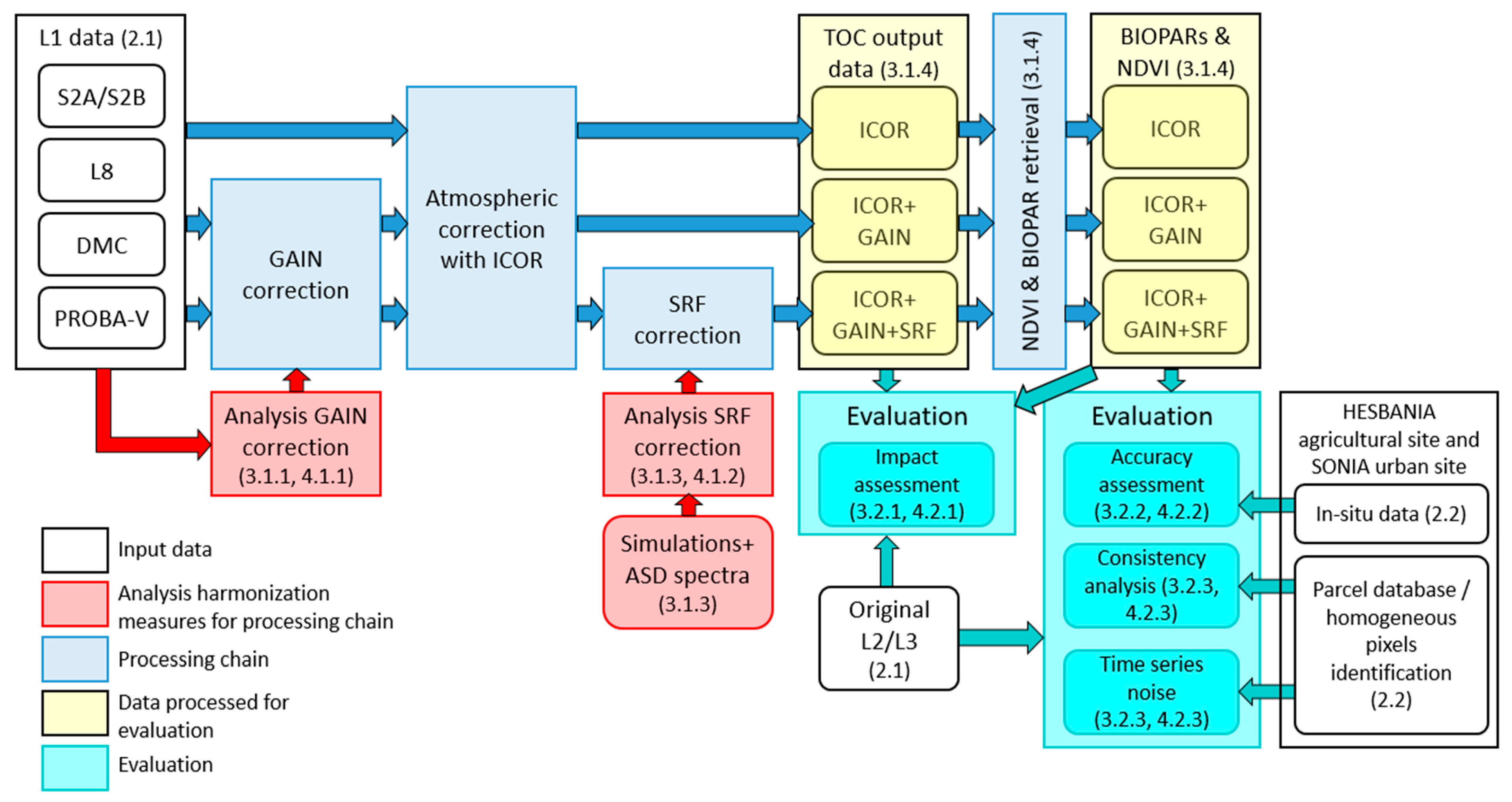
3.1. Harmonisation Approach
3.1.1. L1 TOA Intercalibration
3.1.2. Atmospheric Correction
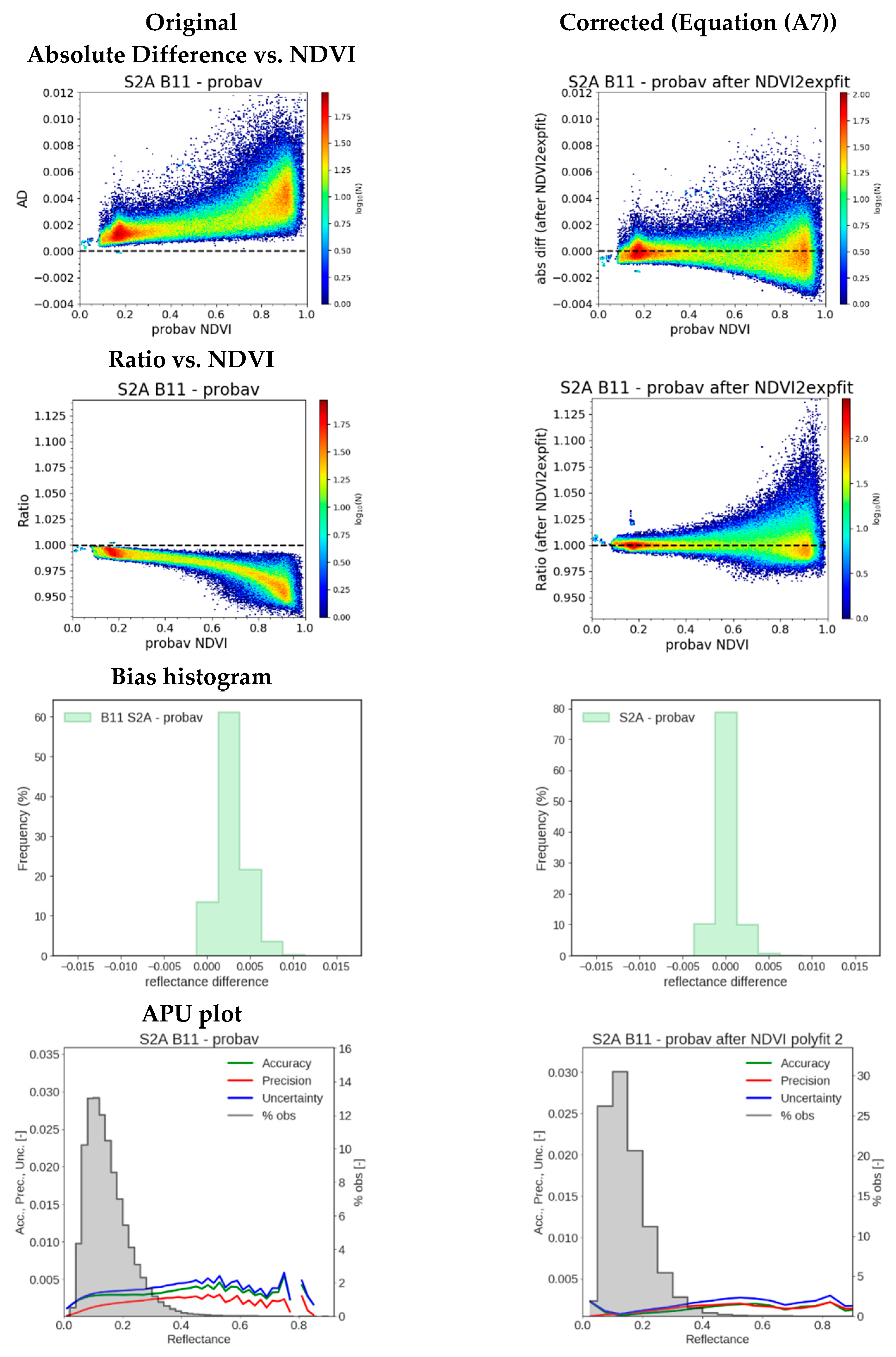
3.1.3. Derivation of Spectral Adjustment Functions
- Shape of the correction function overlaid on a scatterplot of the data. This is only possible if the correction function is based on 1 input parameter, e.g., the NDVI;
- Density scatterplots between the absolute difference (AD) of S1 and S2 (Y-axis) and the NDVI of S1 (X-axis). The majority of the simulations should be centered around an AD value of 0 and this should be stable for the entire NDVI range. Same plot for SBAF, which should be centered around an SBAF value of 1;
- Bias histogram;
- APU plot: the accuracy, precision and uncertainty should be smaller than compared to the comparison of the original data over the reflectance range.
3.1.4. Generation of Enhanced L2 and L3 Products Using a Common Processing Chain
- 8B_BIOPAR: S2 8B_*, L8 5B_* and DMC 3B_*: all the available spectral information is used for the retrieval of the BIOPARs.
- 3B_BIOPAR: S2 3B_*, L8 3B_* and DMC 3B_*: the same spectral information is used for the retrieval of the BIOPARs.
3.2. Evaluation of the Enhanced L2 and L3 Time Series
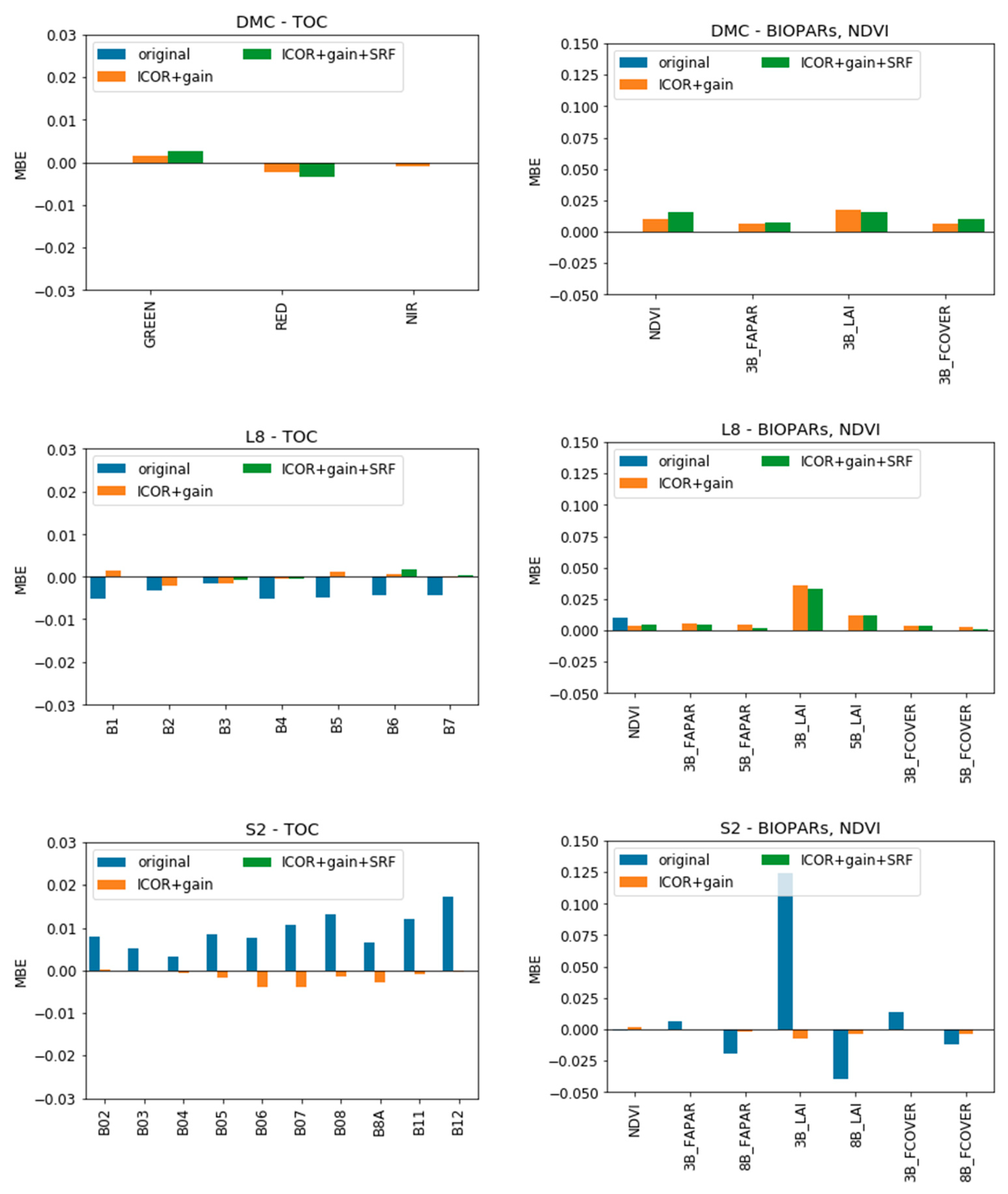
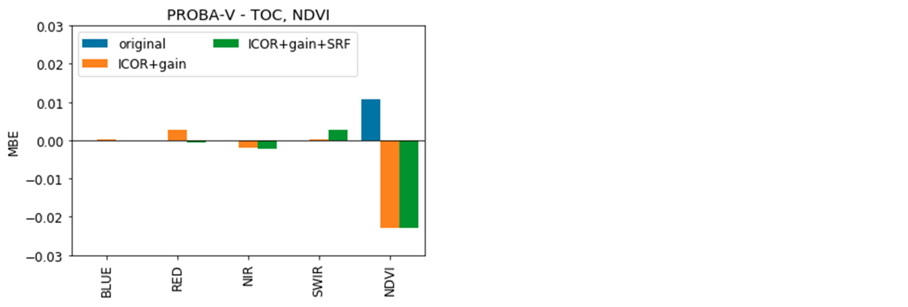
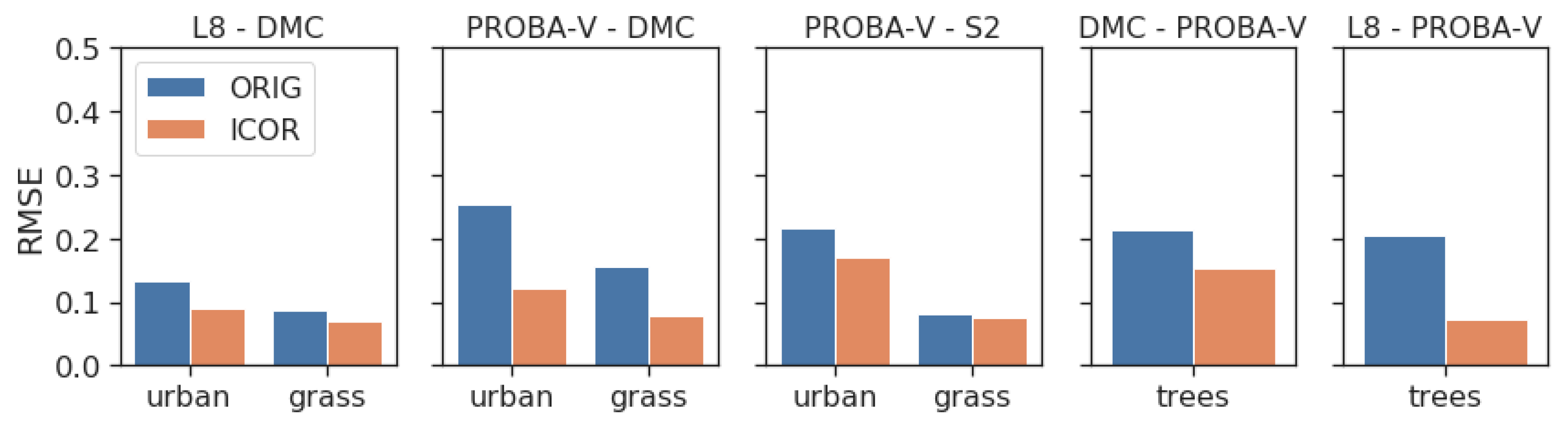
3.2.1. Impact Assessment of the Different Harmonization Measures per Sensor
- ICOR—ICOR + gain
- ICOR—ICOR + gain + SRF
- ICOR—original
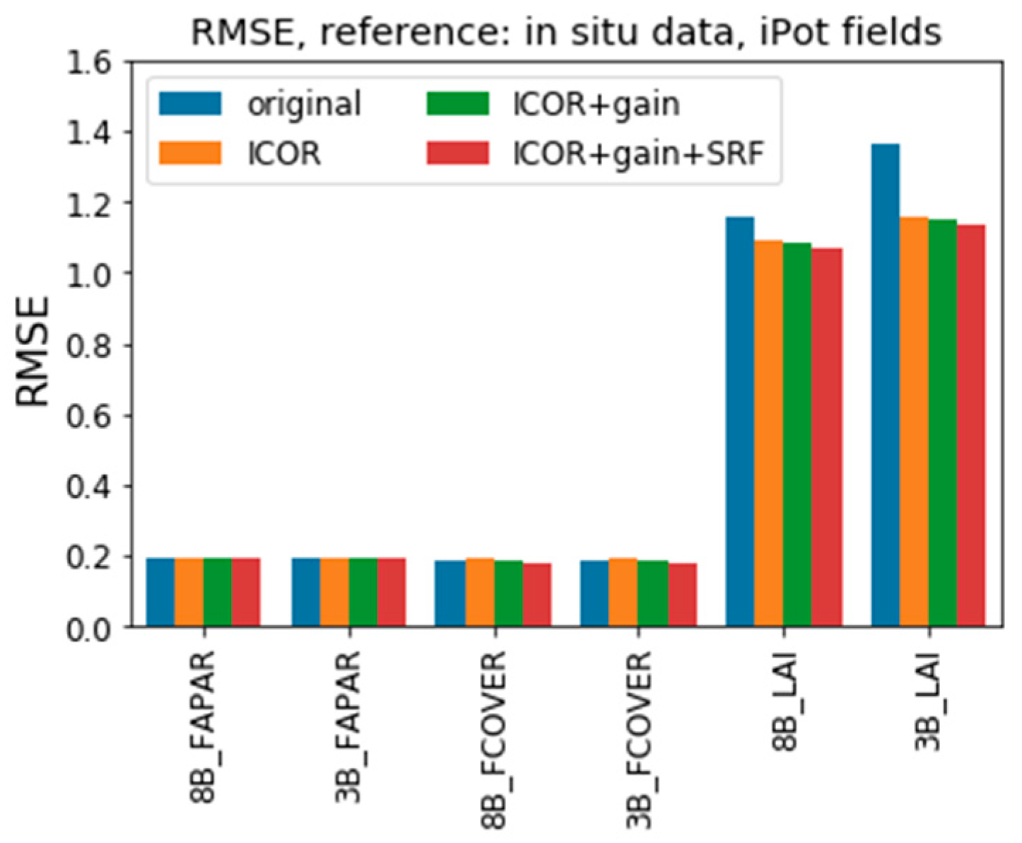
3.2.2. Accuracy Assessment of the Downstream Products against In Situ Data
3.2.3. Consistency Analysis of the Downstream Products
Consistency Analysis with S2A as Reference
Time Series Analyses
4. Results
4.1. Harmonization Approach Results
4.1.1. L1 TOA Intercalibration
4.1.2. Spectral Response Adjustment Functions
4.2. Evaluation of the Enhanced L2 and L3 Time Series
4.2.1. Impact Assessment of the Different Harmonization Measures per Sensor
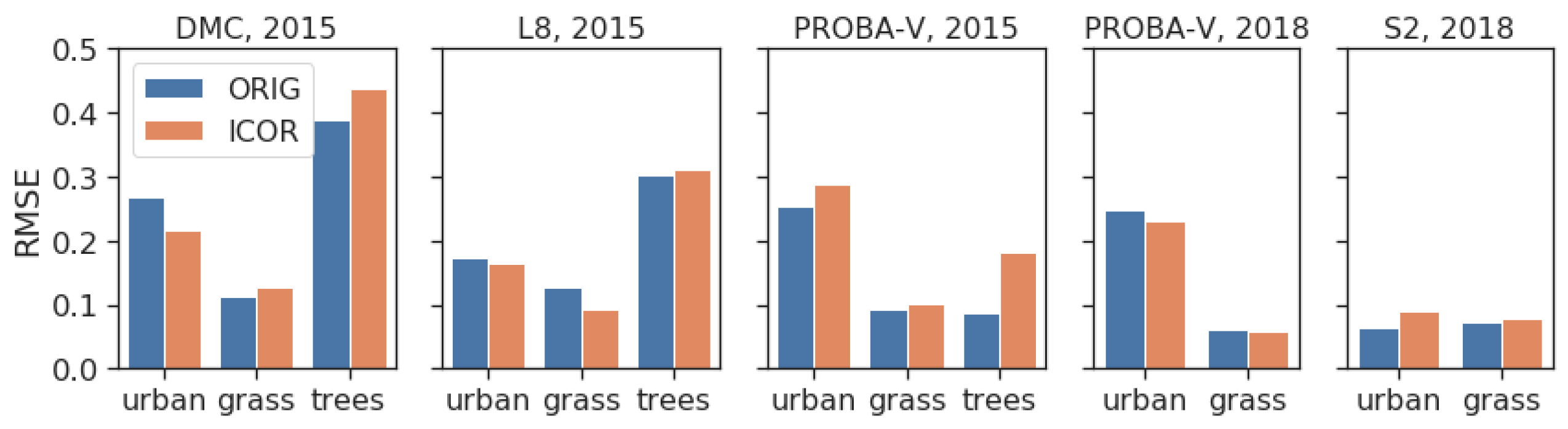
4.2.2. Accuracy Assessment of the Downstream Products against In Situ Data
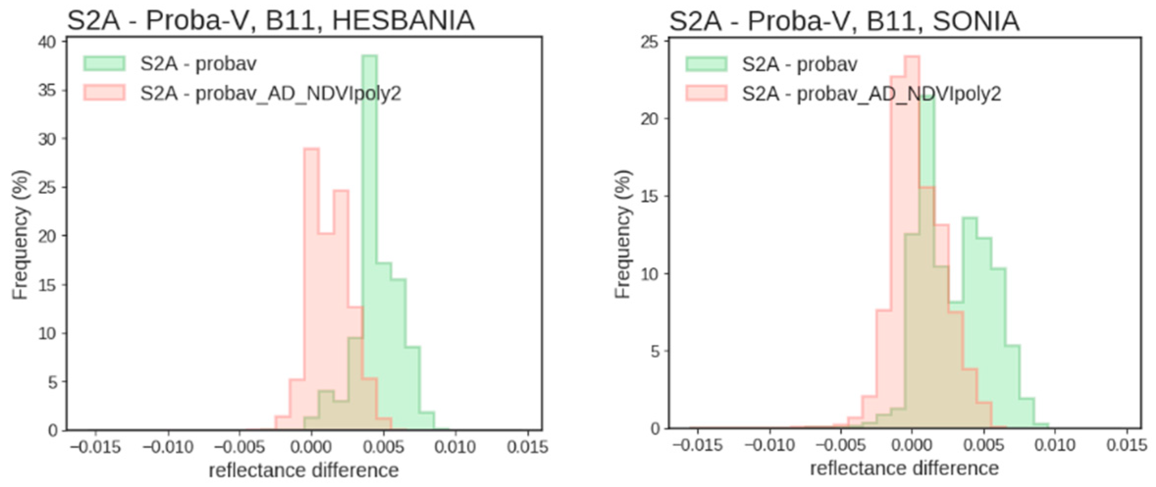
HESBANIA
SONIA
4.2.3. Consistency Analysis of the Downstream Products
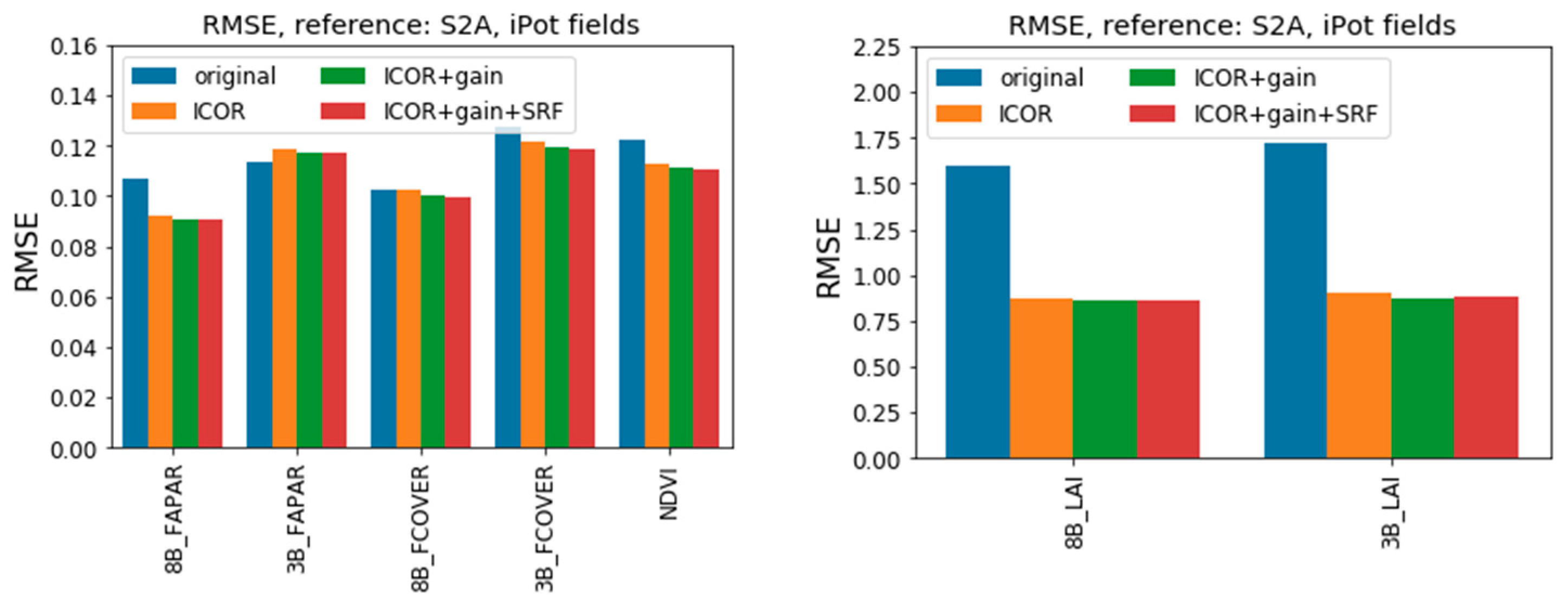
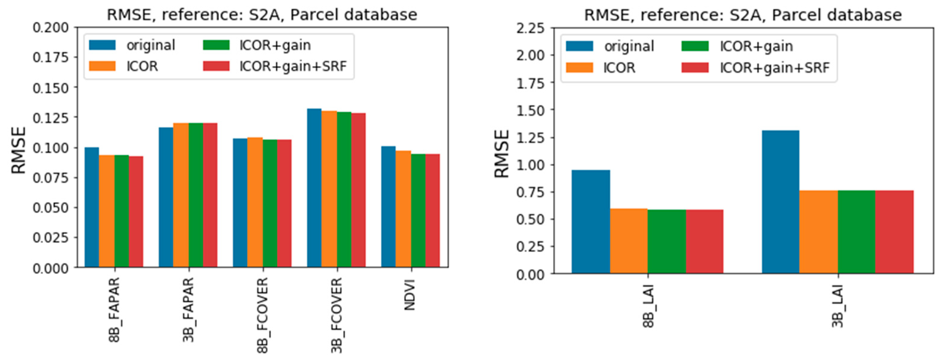
Consistency Analysis with S2A as Reference
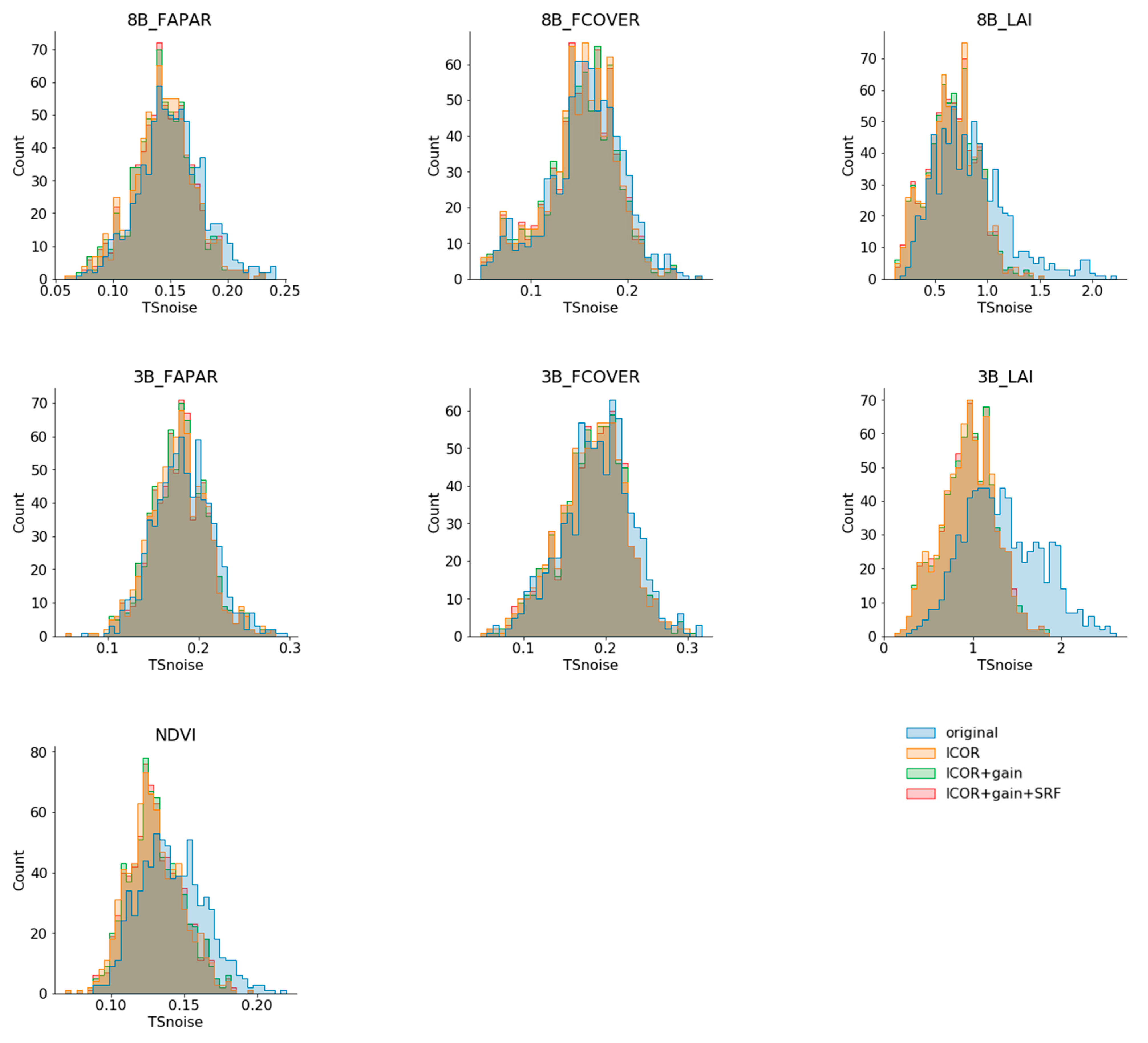
Time Series Analyses
5. Discussion
6. Conclusions
Author Contributions
Funding
Conflicts of Interest
Appendix A. Mathematical Expressions of SRF Correction Functions
References
- Banskota, A.; Kayastha, N.; Falkowski, M.J.; Wulder, M.A.; Froese, R.E.; White, J.C. Forest Monitoring Using Landsat Time Series Data: A Review. Can. J. Remote Sens. 2014, 40, 362–384. [Google Scholar] [CrossRef]
- Gao, F.; Anderson, M.; Daughtry, C.; Johnson, D. Assessing the Variability of Corn and Soybean Yields in Central Iowa Using High Spatiotemporal Resolution Multi-Satellite Imagery. Remote Sens. 2018, 10, 1489. [Google Scholar] [CrossRef] [Green Version]
- Segarra, J.; Buchaillot, M.L.; Araus, J.L.; Kefauver, S.C. Remote Sensing for Precision Agriculture: Sentinel-2 Improved Features and Applications. Agronomy 2020, 10, 641. [Google Scholar] [CrossRef]
- Brezonik, P.; Menken, K.D.; Bauer, M. Landsat-based remote sensing of lake water quality characteristics, including chlorophyll and colored dissolved organic matter (CDOM). Lake Reserv. Manag. 2005, 21, 373–382. [Google Scholar] [CrossRef]
- Fritz, S.; See, L.; Bayas, J.C.L.; Waldner, F.; Jacques, D.; Becker-Reshef, I.; Whitcraft, A.; Baruth, B.; Bonifacio, R.; Crutchfield, J.; et al. A comparison of global agricultural monitoring systems and current gaps. Agric. Syst. 2019, 168, 258–272. [Google Scholar] [CrossRef]
- Rembold, F.; Meroni, M.; Urbano, F.; Csak, G.; Kerdiles, H.; Perez-Hoyos, A.; Lemoine, G.; Leo, O.; Negre, T. ASAP: A new global early warning system to detect anomaly hot spots of agricultural production for food security analysis. Agric. Syst. 2019, 168, 247–257. [Google Scholar] [CrossRef] [PubMed]
- Wulder, M.A.; Hermosilla, T.; White, J.C.; Hobart, G.; Masek, J.G. Augmenting Landsat time series with Harmonized Landsat Sentinel-2 data products: Assessment of spectral correspondence. Sci. Remote Sens. 2021, 4, 100031. [Google Scholar] [CrossRef]
- Weiss, M.; Jacob, F.; Duveiller, G. Remote sensing for agricultural applications: A meta-review. Remote Sens. Environ. 2020, 236, 111402. [Google Scholar] [CrossRef]
- WatchItGrow. Available online: https://vito.be/en/remote-sensing/watchitgrow (accessed on 24 November 2021).
- Beamish, A.; Raynolds, M.K.; Epstein, H.; Frost, G.V.; Macander, M.J.; Bergstedt, H.; Bartsch, A.; Kruse, S.; Miles, V.; Tanis, C.M.; et al. Recent trends and remaining challenges for optical remote sensing of Arctic tundra vegetation: A review and outlook. Remote Sens. Environ. 2020, 246, 111872. [Google Scholar] [CrossRef]
- Wirion, C.; Bauwens, W.; Verbeiren, B. Location- and Time-Specific Hydrological Simulations with Multi-Resolution Remote Sensing Data in Urban Areas. Remote Sens. 2017, 9, 645. [Google Scholar] [CrossRef] [Green Version]
- Bégué, A.; Arvor, D.; Bellon, B.; Betbeder, J.; de Abelleyra, D.; PD Ferraz, R.; Lebourgeois, V.; Lelong, C.; Simões, M.; R Verón, S. Remote Sensing and Cropping Practices: A Review. Remote Sens. 2018, 10, 99. [Google Scholar] [CrossRef] [Green Version]
- Mandanici, E.; Bitelli, G. Preliminary Comparison of Sentinel-2 and Landsat 8 Imagery for a Combined Use. Remote Sens. 2016, 8, 1014. [Google Scholar] [CrossRef] [Green Version]
- Van Leeuwen, W.J.D.; Orr, B.J.; Marsh, S.E.; Herrmann, S.M. Multi-sensor NDVI data continuity: Uncertainties and implications for vegetation monitoring applications. Remote Sens. Environ. 2006, 100, 67–81. [Google Scholar] [CrossRef]
- Claverie, M.; Ju, J.; Masek, J.G.; Dungan, J.L.; Vermote, E.F.; Roger, J.C.; Skakun, S.V.; Justice, C. The Harmonized Landsat and Sentinel-2 surface reflectance data set. Remote Sens. Environ. 2018, 219, 145–161. [Google Scholar] [CrossRef]
- Saunier, S.; Louis, J.; Debaecker, V.; Beaton, T.; Cadau, E.G.; Boccia, V.; Gascon, F. Sen2like, A Tool To Generate Sentinel-2 Harmonised Surface Reflectance Products—First Results with Landsat-8. In Proceedings of the IEEE IGARSS 2019—2019 IEEE International Geoscience and Remote Sensing Symposium, Yokohama, Japan, 28 July–2 August 2019; IEEE: Piscataway, NJ, USA,; pp. 5650–5653. [Google Scholar]
- Helder, D.; Markham, B.; Morfitt, R.; Storey, J.; Barsi, J.; Gascon, F.; Clerc, S.; LaFrance, B.; Masek, J.; Roy, D.; et al. Observations and Recommendations for the Calibration of Landsat 8 OLI and Sentinel 2 MSI for Improved Data Interoperability. Remote Sens. 2018, 10, 1340. [Google Scholar] [CrossRef] [Green Version]
- Barsi, J.A.; Alhammoud, B.; Czapla-Myers, J.; Gascon, F.; Haque, M.O.; Kaewmanee, M.; Leigh, L.; Markham, B.L. Sentinel-2A MSI and Landsat-8 OLI radiometric cross comparison over desert sites. Eur. J. Remote Sens. 2018, 51, 822–837. [Google Scholar] [CrossRef]
- Jing, X.; Leigh, L.; Teixeira Pinto, C.; Helder, D. Evaluation of RadCalNet Output Data Using Landsat 7, Landsat 8, Sentinel 2A, and Sentinel 2B Sensors. Remote Sens. 2019, 11, 541. [Google Scholar] [CrossRef] [Green Version]
- Alhammoud, B.; Jackson, J.; Clerc, S.; Arias, M.; Bouzinac, C.; Gascon, F.; Cadau, E.G.; Iannone, R.Q.; Boccia, V. Sentinel-2 Level-1 Radiometry Assessment Using Vicarious Methods from DIMITRI Toolbox and Field Measurements from RadCalNet Database. IEEE J. Sel. Top. Appl. Earth Obs. Remote Sens. 2019, 12, 3470–3479. [Google Scholar] [CrossRef]
- Lamquin, N.; Woolliams, E.; Bruniquel, V.; Gascon, F.; Gorroño, J.; Govaerts, Y.; Leroy, V.; Lonjou, V.; Alhammoud, B.; Barsi, J.A.; et al. An inter-comparison exercise of Sentinel-2 radiometric validations assessed by independent expert groups. Remote Sens. Environ. 2019, 233, 111369. [Google Scholar] [CrossRef]
- Swinnen, E.; Veroustraete, F. Extending the SPOT-VEGETATION NDVI time series (1998–2006) back in time with NOAA-AVHRR data (1985–1998) for Southern Africa. IEEE Trans. Geosci. Remote Sens. 2008, 46, 558–572. [Google Scholar] [CrossRef]
- Pahlevan, N.; Sarkar, S.; Franz, B.A.; Balasubramanian, S.V.; He, J. Sentinel-2 MultiSpectral Instrument (MSI) data processing for aquatic science applications: Demonstrations and validations. Remote Sens. Environ. 2017, 201, 47–56. [Google Scholar] [CrossRef]
- León-Tavares, J.; Roujean, J.-L.; Smets, B.; Wolters, E.; Toté, C.; Swinnen, E. Correction of Directional Effects in VEGETATION NDVI Time-Series. Remote Sens. 2021, 13, 1130. [Google Scholar] [CrossRef]
- D’Odorico, P.; Gonsamo, A.; Damm, A.; Schaepman, M.E. Experimental evaluation of sentinel-2 spectral response functions for NDVI time-series continuity. IEEE Trans. Geosci. Remote Sens. 2013, 51, 1336–1348. [Google Scholar] [CrossRef]
- Gonsamo, A.; Chen, J.M. Spectral response function comparability among 21 satellite sensors for vegetation monitoring. IEEE Trans. Geosci. Remote Sens. 2013, 51, 1319–1335. [Google Scholar] [CrossRef]
- Trishchenko, A.P.; Cihlar, J.; Li, Z. Effects of spectral response function on surface reflectance and NDVI measured with moderate resolution satellite sensors. Remote Sens. Environ. 2002, 81, 1–18. [Google Scholar] [CrossRef]
- Villaescusa-Nadal, J.L.; Franch, B.; Roger, J.-C.C.; Vermote, E.F.; Skakun, S.; Justice, C. Spectral Adjustment Model’s Analysis and Application to Remote Sensing Data. IEEE J. Sel. Top. Appl. Earth Obs. Remote Sens. 2019, 12, 961–972. [Google Scholar] [CrossRef]
- Chander, G.; Mishra, N.; Helder, D.L.; Aaron, D.B.; Angal, A.; Choi, T.; Xiong, X.; Doelling, D.R. Applications of spectral band adjustment factors (SBAF) for cross-calibration. IEEE Trans. Geosci. Remote Sens. 2013, 51, 1267–1281. [Google Scholar] [CrossRef]
- Belair. Available online: https://belair.vito.be/ (accessed on 23 November 2021).
- Dierckx, W.; Sterckx, S.; Benhadj, I.; Livens, S.; Duhoux, G.; Van Achteren, T.; Francois, M.; Mellab, K.; Saint, G. PROBA-V mission for global vegetation monitoring: Standard products and image quality. Int. J. Remote Sens. 2014, 35, 2589–2614. [Google Scholar] [CrossRef]
- PROBA-V. Available online: https://proba-v.vgt.vito.be (accessed on 24 November 2021).
- RAHMAN, H.; DEDIEU, G. SMAC: A simplified method for the atmospheric correction of satellite measurements in the solar spectrum. Int. J. Remote Sens. 1994, 15, 123–143. [Google Scholar] [CrossRef]
- Toté, C.; Swinnen, E.; Sterckx, S.; Adriaensen, S.; Benhadj, I.; Iordache, M.-D.; Bertels, L.; Kirches, G.; Stelzer, K.; Dierckx, W.; et al. Evaluation of PROBA-V Collection 1: Refined Radiometry, Geometry, and Cloud Screening. Remote Sens. 2018, 10, 1375. [Google Scholar] [CrossRef] [Green Version]
- Pisabarro, P.; Carballo, M.; Iturri, A.; Bueno, I.; Mazzoleni, A.; Luengo, M.; Bravo, F.A.; Santos, J.A.; Pirondini, F. Satellite Operations Strategies and Experience in DEIMOS-1 and DEIMOS-2 Missions. In Proceedings of the SpaceOps 2016 Conference, Daejeon, Korea, 16–20 May 2016; American Institute of Aeronautics and Astronautics: Reston, VA, USA, 2016. [Google Scholar]
- Richter, R. Atmospheric correction of DAIS hyperspectral image data. Comput. Geosci. 1996, 22, 785–793. [Google Scholar] [CrossRef]
- Drusch, M.; Del Bello, U.; Carlier, S.; Colin, O.; Fernandez, V.; Gascon, F.; Hoersch, B.; Isola, C.; Laberinti, P.; Martimort, P.; et al. Sentinel-2: ESA’s Optical High-Resolution Mission for GMES Operational Services. Remote Sens. Environ. 2012, 120, 25–36. [Google Scholar] [CrossRef]
- Gascon, F.; Bouzinac, C.; Thépaut, O.; Jung, M.; Francesconi, B.; Louis, J.; Lonjou, V.; Lafrance, B.; Massera, S.; Gaudel-Vacaresse, A.; et al. Copernicus Sentinel-2A Calibration and Products Validation Status. Remote Sens. 2017, 9, 584. [Google Scholar] [CrossRef] [Green Version]
- Sentinel-2. Available online: https://sentinel.esa.int/web/sentinel/missions/sentinel-2 (accessed on 24 November 2021).
- Main-Knorn, M.; Pflug, B.; Louis, J.; Debaecker, V.; Müller-Wilm, U.; Gascon, F. Sen2Cor for Sentinel-2. In Proceedings of the Image and Signal Processing for Remote Sensing XXIII, International Society for Optics and Photonics, Warsaw, Poland, 4 October 2017; Bruzzone, L., Bovolo, F., Benediktsson, J.A., Eds.; SPIE: Bellingham, WA, USA, 2017; p. 3. [Google Scholar]
- Terrascope. Available online: https://terrascope.be/ (accessed on 24 November 2021).
- USGS Landsat Collections. Available online: https://www.usgs.gov/core-science-systems/nli/landsat/landsat-collection-1?qt-science_support_page_related_con=1#qt-science_support_page_related_con (accessed on 24 November 2021).
- Vermote, E.; Justice, C.; Claverie, M.; Franch, B. Preliminary analysis of the performance of the Landsat 8/OLI land surface reflectance product. Remote Sens. Environ. 2016, 185, 46–56. [Google Scholar] [CrossRef]
- Weiss, M.; Baret, F. S2ToolBox Level 2 products: LAI, FAPAR, FCOVER—Version 1.1; INRAE: Paris, France, 2016. [Google Scholar]
- Govaerts, Y.; Sterckx, S.; Adriaensen, S. Use of simulated reflectances over bright desert target as an absolute calibration reference. Remote Sens. Lett. 2013, 4, 523–531. [Google Scholar] [CrossRef]
- Sterckx, S.; Wolters, E. Radiometric Top-of-Atmosphere Reflectance Consistency Assessment for Landsat 8/OLI, Sentinel-2/MSI, PROBA-V, and DEIMOS-1 over Libya-4 and RadCalNet Calibration Sites. Remote Sens. 2019, 11, 2253. [Google Scholar] [CrossRef] [Green Version]
- Holben, B.N.; Eck, T.F.; Slutsker, I.; Tanré, D.; Buis, J.P.; Setzer, A.; Vermote, E.; Reagan, J.A.; Kaufman, Y.J.; Nakajima, T.; et al. AERONET—A federated instrument network and data archive for aerosol characterization. Remote Sens. Environ. 1998, 66, 1–16. [Google Scholar] [CrossRef]
- De Keukelaere, L.; Sterckx, S.; Adriaensen, S.; Knaeps, E.; Reusen, I.; Giardino, C.; Bresciani, M.; Hunter, P.; Neil, C.; Van der Zande, D.; et al. Atmospheric correction of Landsat-8/OLI and Sentinel-2/MSI data using iCOR algorithm: Validation for coastal and inland waters. Eur. J. Remote Sens. 2018, 51, 525–542. [Google Scholar] [CrossRef] [Green Version]
- Wolters, E.; Tot, C.; Sterckx, S.; Adriaensen, S.; Henocq, C.; Scifoni, S.; Dransfeld, S. iCOR Atmospheric Correction on Sentinel-3/OLCI over Land: Intercomparison with AERONET, RadCalNet, and SYN Level-2. Remote Sens. 2021, 13, 654. [Google Scholar] [CrossRef]
- Doxani, G.; Vermote, E.; Roger, J.-C.; Gascon, F.; Adriaensen, S.; Frantz, D.; Hagolle, O.; Hollstein, A.; Kirches, G.; Li, F.; et al. Atmospheric Correction Inter-Comparison Exercise. Remote Sens. 2018, 10, 352. [Google Scholar] [CrossRef] [Green Version]
- Berk, A.; Anderson, G.P.; Acharya, P.K.; Bernstein, L.S.; Muratov, L.; Lee, J.; Fox, M.; Adler-Golden, S.M.; Chetwynd, J.H., Jr.; Hoke, M.L.; et al. MODTRAN5: 2006 update. In SPIE 6233, Algorithms and Technologies for Multispectral, Hyperspectral, and Ultraspectral Imagery XII; Shen, S.S., Lewis, P.E., Eds.; SPIE: Bellingham, WA, USA, 2006; p. 62331F. [Google Scholar]
- Teillet, P.M.; Fedosejevs, G.; Thome, K.J.; Barker, J.L. Impacts of spectral band difference effects on radiometric cross-calibration between satellite sensors in the solar-reflective spectral domain. Remote Sens. Environ. 2007, 110, 393–409. [Google Scholar] [CrossRef]
- VERHOEF, W.; BACH, H. Coupled soil–leaf-canopy and atmosphere radiative transfer modeling to simulate hyperspectral multi-angular surface reflectance and TOA radiance data. Remote Sens. Environ. 2007, 109, 166–182. [Google Scholar] [CrossRef]
- Darvishzadeh, R.; Skidmore, A.; Schlerf, M.; Atzberger, C.; Corsi, F.; Cho, M. LAI and chlorophyll estimation for a heterogeneous grassland using hyperspectral measurements. ISPRS J. Photogramm. Remote Sens. 2008, 63, 409–426. [Google Scholar] [CrossRef]
- Mousivand, A.; Menenti, M.; Gorte, B.; Verhoef, W. Global sensitivity analysis of the spectral radiance of a soil-vegetation system. Remote Sens. Environ. 2014, 145, 131–144. [Google Scholar] [CrossRef]
- Steven, M.D.; Malthus, T.J.; Baret, F.; Xu, H.; Chopping, M.J. Intercalibration of vegetation indices from different sensor systems. Remote Sens. Environ. 2003, 88, 412–422. [Google Scholar] [CrossRef]
- TRISHCHENKO, A. Effects of spectral response function on surface reflectance and NDVI measured with moderate resolution satellite sensors: Extension to AVHRR NOAA-17, 18 and METOP-A. Remote Sens. Environ. 2009, 113, 335–341. [Google Scholar] [CrossRef]
- WEISS, M.; BARET, F.; GARRIGUES, S.; LACAZE, R. LAI and fAPAR CYCLOPES global products derived from VEGETATION. Part 2: Validation and comparison with MODIS collection 4 products. Remote Sens. Environ. 2007, 110, 317–331. [Google Scholar] [CrossRef]
- Vermote, E.; Justice, C.O.; Bréon, F.M. Towards a generalized approach for correction of the BRDF effect in MODIS directional reflectances. IEEE Trans. Geosci. Remote Sens. 2009, 47, 898–908. [Google Scholar] [CrossRef]
- Revel, C.; Lonjou, V.; Marcq, S.; Desjardins, C.; Fougnie, B.; Coppolani-Delle Luche, C.; Guilleminot, N.; Lacamp, A.S.; Lourme, E.; Miquel, C.; et al. Sentinel-2A and 2B absolute calibration monitoring. Eur. J. Remote Sens. 2019, 52, 122–137. [Google Scholar] [CrossRef] [Green Version]
- Lozano, F.J.; Romo, A.; Moclan, C.; Gil, J.; Pirondini, F. The DEIMOS-1 mission: Absolute and relative calibration activities and radiometric optimisation. In Proceedings of the 2012 IEEE International Geoscience and Remote Sensing Symposium, Munich, Germany, 22–27 July 2012; pp. 4754–4757. [Google Scholar]
- PROBA-V Radiometric Calibration. Available online: https://proba-v.vgt.vito.be/en/quality/radiometric/radiometric-calibration (accessed on 10 February 2022).
- Landsat 8 Calibration Updates. Available online: https://www.usgs.gov/landsat-missions/landsat-8-oli-and-tirs-calibration-notices (accessed on 10 February 2022).
- Sentinel-2 Quality Reports. Available online: https://sentinel.esa.int/web/sentinel/user-guides/sentinel-2-msi/document-library (accessed on 10 February 2022).
- Zhang, H.K.; Roy, D.P.; Yan, L.; Li, Z.; Huang, H.; Vermote, E.; Skakun, S.; Roger, J.C. Characterization of Sentinel-2A and Landsat-8 top of atmosphere, surface, and nadir BRDF adjusted reflectance and NDVI differences. Remote Sens. Environ. 2018, 215, 482–494. [Google Scholar] [CrossRef]
- Roy, D.; Li, Z.; Zhang, H. Adjustment of Sentinel-2 Multi-Spectral Instrument (MSI) Red-Edge Band Reflectance to Nadir BRDF Adjusted Reflectance (NBAR) and Quantification of Red-Edge Band BRDF Effects. Remote Sens. 2017, 9, 1325. [Google Scholar] [CrossRef] [Green Version]
- Franch, B.; Vermote, E.; Skakun, S.; Roger, J.-C.; Masek, J.; Ju, J.; Villaescusa-Nadal, J.; Santamaria-Artigas, A. A Method for Landsat and Sentinel 2 (HLS) BRDF Normalization. Remote Sens. 2019, 11, 632. [Google Scholar] [CrossRef] [Green Version]


| Sentinel-2 | Landsat 8 | DMC | PROBA-V |
|---|---|---|---|
| B3 543–578 | B3 533–590 | GREEN 520–600 | |
| B4 650–680 | B4 636–673 | RED 630–690 | B2 614–696 |
| B5 698–713 | |||
| B6 733–748 | |||
| B7 773–793 | |||
| B8 785–899 | B5 851–879 | NIR 770–900 | B3 772–902 |
| B8A 855–875 | B5 851–879 | NIR 770–900 | B3 772–902 |
| B11 1565–1655 | B6 1566–1651 | SWIR 1570–1635 | |
| B12 2100–2280 | B7 2107–2294 |
| Dataset Name | Processing Performed |
|---|---|
| Nominal/original baseline level2 products | |
| ORIG | Original data, processing performed with Sen2COR (for S2), LaSRC (for L8), SMAC (for PROBA-V) |
| Belharmony processing | |
| ICOR | Atmospheric correction completed with ICOR |
| ICOR + GAIN | Gain applied to TOA radiance data + atmospheric correction performed with ICOR |
| ICOR + GAIN + SRF | Gain applied to TOA radiance data + atmospheric correction performed with ICOR + SRF correction |
| Name of Resulting Time Series | S2A | S2B | L8 | DMC |
|---|---|---|---|---|
| ICOR | ICOR | ICOR | ICOR | ICOR |
| ICOR + gain | ICOR | ICOR + gain | ICOR + gain | ICOR + gain |
| ICOR + gain + SRF | ICOR | ICOR + gain | ICOR + gain + SRF | ICOR + gain + SRF |
| Original | Original | Original | ICOR | ICOR |
| Class | Label | DMC | S2 | L8 | Proba-V |
|---|---|---|---|---|---|
| NDVI: urban impervious | Urban | 2015 | 2018 | 2015 and 2018 | 2015 and 2018 |
| NDVI: urban grass | Grass | 2015 | 2018 | 2015 and 2018 | 2015 and 2018 |
| LAI: urban trees | Trees | 2015 | 2018 | 2015 and 2018 | 2015 and 2018 |
| S2 | S2 | S2A | %Diff S2B | L8 | L8 | %Diff L8 | DMC | DMC | %Diff DMC | PV | PV | %Diff PV |
|---|---|---|---|---|---|---|---|---|---|---|---|---|
| band | cwv | ratio | vs. S2A | band | cwv | vs. S2A | band | cwv | vs. S2A | band | cwv | vs. S2A |
| 1 | 443 | 1.008 | −1.05% | CA | 443 | −1.05% | Blue | 460 | −1.30% | |||
| 2 | 490 | 0.985 | −0.03% | Blue | 492 | 0.94% | 460 | 0.97% | ||||
| 3 | 560 | 0.999 | −0.16% | Green | 561 | 0.82% | Green | 549 | −3.5% | |||
| 4 | 665 | 1.005 | −0.76% | Red | 654 | 0.08% | Red | 679 | 0.2% | Red | 658 | −1.55% |
| 5 | 705 | 1.016 | −1.32% | |||||||||
| 6 | 740 | 1.023 | −1.49% | |||||||||
| 7 | 783 | 1.034 | −1.35% | |||||||||
| 8 | 842 | 0.999 | −0.40% | NIR | 803 | 0.8% | NIR | 834 | 0.78% | |||
| 8A | 865 | 1.027 | −0.84% | NIR | 865 | −0.28% | ||||||
| 9 | 945 | NA | NA | |||||||||
| 10 | 1375 | NA | NA | Cirrus | 1373 | NA | ||||||
| 11 | 1610 | 0.998 | −0.40% | SWIR1 | 1610 | −0.30% | SWIR | 1610 | −0.21% | |||
| 12 | 2190 | 0.973 | −0.12% | SWIR2 | 2200 | 0.28% |
| Input | S2 | Equation | Coefficients | |||||
|---|---|---|---|---|---|---|---|---|
| band | Band | a | b | c | d | e | f | |
| Landsat-8 | ||||||||
| B3 | B3 | A6 | 1.007457 | 0.007411 | −0.061680 | 0 | - | - |
| B4 | B4 | A6 | 0.983784 | −0.054115 | 0.171154 | −0.030599 | - | - |
| B5 | B8 | No suitable correction found, SRFs too different. | ||||||
| B5 | B8A | Original bands are already very similar | ||||||
| B6 | B11 | A10 | 0.000449 | 4.081912 | −0.954106 | 4.081850 | 0.954195 | - |
| B7 | B12 | A5 | 0.000369 | 0.000779 | −0.020686 | 0.019961 | −0.000708 | 1.000709 |
| DMC | ||||||||
| B1 | B3 | A6 | 1.026747 | 0.023303 | −0.165327 | 0 | - | |
| B2 | B4 | A6 | 0.996053 | −0.037969 | 0.091627 | 0.063597 | ||
| B3 | B8 | Original bands are already very similar | ||||||
| B3 | B8A | No suitable correction found, SRFs too different. | ||||||
| PROBA-V | ||||||||
| B2 | B4 | A6 | 0.993998 | −0.126106 | 0.338988 | 0 | - | |
| B3 | B8 | A9 | 0.999468 | 3.211558 | −1.000562 | 3.2107839 | 1.003200 | |
| B3 | B8A | No suitable correction found, SRFs too different. | ||||||
| SWIR | B11 | A7 | 0.001377 | −0.000669 | 0.004392 | 0 | - | |
Publisher’s Note: MDPI stays neutral with regard to jurisdictional claims in published maps and institutional affiliations. |
© 2022 by the authors. Licensee MDPI, Basel, Switzerland. This article is an open access article distributed under the terms and conditions of the Creative Commons Attribution (CC BY) license (https://creativecommons.org/licenses/by/4.0/).
Share and Cite
Swinnen, E.; Sterckx, S.; Wirion, C.; Verbeiren, B.; Wens, D. Harmonization of Multi-Mission High-Resolution Time Series: Application to BELAIR. Remote Sens. 2022, 14, 1163. https://doi.org/10.3390/rs14051163
Swinnen E, Sterckx S, Wirion C, Verbeiren B, Wens D. Harmonization of Multi-Mission High-Resolution Time Series: Application to BELAIR. Remote Sensing. 2022; 14(5):1163. https://doi.org/10.3390/rs14051163
Chicago/Turabian StyleSwinnen, Else, Sindy Sterckx, Charlotte Wirion, Boud Verbeiren, and Dieter Wens. 2022. "Harmonization of Multi-Mission High-Resolution Time Series: Application to BELAIR" Remote Sensing 14, no. 5: 1163. https://doi.org/10.3390/rs14051163
APA StyleSwinnen, E., Sterckx, S., Wirion, C., Verbeiren, B., & Wens, D. (2022). Harmonization of Multi-Mission High-Resolution Time Series: Application to BELAIR. Remote Sensing, 14(5), 1163. https://doi.org/10.3390/rs14051163