Following the publication of the article [1], it was discovered that the computation of the inpainting Structural Similarity Index (SSIM) metric value was incorrect. However, the relationship between method performances remains unchanged upon correction and all of the conclusions made in the original manuscript still stand.
The issue was related to the following line, where masked SSIM is computed:
| i_ssim_val = ssim(s2_out[mask == mask.min()], |
| s2_gt[mask == mask.min()], |
| multichannel=True) |
Indexing a 3-channel two-dimensional image of 256 by 256 pixels in the above manner returns a spatially flattened array with 3 channels. This does not raise any Python error messages, since the scikit-image function for SSIM computation [2] accepts both two-dimensional and one-dimensional signals. The spatially flattened array with 3 channels results in the use of a single-dimensional kernel by the function, which is inconsistent with the description of SSIM computation in [1], where a two-dimensional 11 × 11 kernel is defined. Instead, the correct procedure to compute inpainting SSIM should be:
| whole_ssim, ssim_img = ssim(s2_gt, |
| s2_out, |
| multichannel = True, |
| full = True) |
| i_ssim_val = ssim_img[mask == mask.min()].mean() |
Based on this change, the following updates to the paper are:
- Figure 2 caption delete duplicate explanation “(c) multi-source residual”
- Figure 4 SSIM values
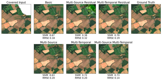 Figure 4. Comparison of DIP-based Synthesis Approaches. Median score samples from 4 repeated runs are shown. Metric values are given for the inpainting region.
 - Figure 5 SSIM of inpainted Region (purple trace)
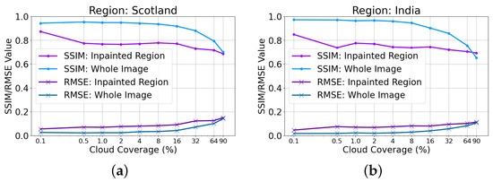 Figure 5. SSIM and RMSE plots for the cloud coverage sweeps for MS-MT mode for (a) Scotland Region (b) India Region.
 - Figure 6 SSIM values
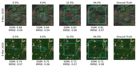 Figure 6. Samples of images reconstructed in the cloud coverage sweep procedure (ranging from 0.5% to 64.0% cloud cover) for MS-MT mode in Scotland (top row) and India (bottom row). The SSIM and RMSE metric values are shown for the inpainted region.
 - Table 2 Inpainting SSIM
 Table 2. MS—Multi-Source (Sentinel 1), MT—Multi-Temporal, -R—Residual Variants. Optimal performance maximizes SSIM and minimizes RMSE. This occurs for the modes using temporal support data, with the MS-MT mode surpassing all other for both dataset and both for the inpainting region and the whole image.
 - The sentence in line 257 should read “The inpainting quality appears to be consistent for cloud coverage ratio between 0.1% to 16%, where the inpainted region SSIM is approximately 0.75 for the Scotland and India regions.”
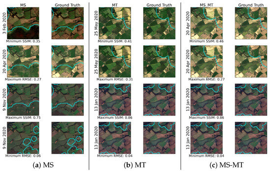 Figure 9. Reconstructions with the lowest (top two rows) and highest (bottom two rows) performance for both SSIM and RMSE for the Scotland region. Each row contains all three stacked modes (MS, MT, and MS-MT).
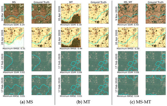 Figure 10. Reconstructions with the lowest (top two rows) and highest (bottom two rows) performance for both SSIM and RMSE for the India region. Each row contains all three stacked modes (MS, MT, and MS-MT).
- Sentence in line 355 should read “The multi-temporal and multi-source (MS-MT) mode offers the highest performance of the three evaluated modes with an average SSIM greater than 0.87 and 0.64 for the whole image and inpainting regions, respectively.”
The authors apologize for any inconvenience caused and state that the scientific conclusions are unaffected. This correction was approved by the Academic Editor. The original publication has also been updated.
References
- Czerkawski, M.; Upadhyay, P.; Davison, C.; Werkmeister, A.; Cardona, J.; Atkinson, R.; Michie, C.; Andonovic, I.; Macdonald, M.; Tachtatzis, C. Deep Internal Learning for Inpainting of Cloud-Affected Regions in Satellite Imagery. Remote Sens. 2022, 14, 1342. [Google Scholar] [CrossRef]
- Module: Metrics. Available online: https://scikit-image.org/docs/dev/api/skimage.metrics.html#skimage.metrics.structural_similarity (accessed on 19 May 2022).
Publisher’s Note: MDPI stays neutral with regard to jurisdictional claims in published maps and institutional affiliations. |
© 2022 by the authors. Licensee MDPI, Basel, Switzerland. This article is an open access article distributed under the terms and conditions of the Creative Commons Attribution (CC BY) license (https://creativecommons.org/licenses/by/4.0/).