Glacial Outburst Floods Responsible for Major Environmental Shift in Arctic Coastal Catchment, Rekvedbukta, Albert I Land, Svalbard

Abstract

Small Arctic coastal catchments and coastal lagoon systems are some of the most vulnerable to climate change. Glacial retreat and the development of glacial lakes and drainage systems provide opportunities for hazardous events such as GLOFs. We observe that the stability of lagoons and their associated barriers are controlled by the frequency and magnitude of storms approaching the coasts, access to sediment supplies and resilience to sea-level rise. Based on multidecadal remote sensing data, we were able to identify the rate of glacial recession, the development of glacial lakes, vegetation response to climate change and a GLOF event, and shoreline and lagoon responses to the environmental shifts within the small catchment. Here we present an example of lagoon system evolution where a glacial outburst flood exerted significant control over lagoon drainage and coastal barrier stability.

1. Introduction

Climate change is particularly visible in the Arctic, which is reinforced by so-called Arctic amplification and has warmed nearly four times faster than the global average [1]. This is especially noticeable with regards to the rapid loss of snow cover, which has been reduced by about half since the summer of 1979, and with respect to the amount of sea ice, which has decreased by 80% since the 1980s [2]. At the same time, there has been an accelerated recession of glaciers and major changes in the thermal state of permafrost [3]. In the small catchments (here defined as <10 km²), environmental changes, i.e., glacier retreat, geomorphological process activation [4], shorter snow cover occurrence or vegetation expansion, and longer melting seasons [5], are rapidly becoming visible. With the ongoing glacial retreat since the Little Ice Age maximum, glacial lakes are being formed, and drainage systems are developing to form the new proglacial landscapes. Deepening of the active layer has been observed [5], showing the increase in geomorphological activity to be visible. These factors highlight the importance of research in small catchments as these areas are fragile and can quickly shift from the glacial to the paraperiglacial type.

Arctic coasts are extremely vulnerable to climate change [6], with the influence of warmer temperatures on the functioning of coastal zones having been seen to be profound [4,5,6]. Changes occurring in warmer Arctic lands and seas concentrate in the coastal zones [7], resulting in, i.a., increased coastal erosion [8,9]. Additionally, the lack of sea ice, which plays a protective role [10], results in an increase in the length of the wind path. This means more energy is transmitted to the waves, which in turn enhances their erosional capabilities [11]. The majority of studies, however, refers to mid-latitude and tropical coastal zones with only limited insight into Arctic lagoon responses. Here we present the first remotely sensed proof showing that significant control of lagoon drainage and coastal barrier stability can be exerted by glacial outburst floods from local rapidly retreating glaciers. It is important to mention that over the last few decades, most of the coastal research has focused on mechanisms controlling the evolution of the ice-rich permafrost coasts of Alaska, Yukon or Siberia, whereas less attention has been paid to still glaciated parts of the regions such as the Canadian Arctic Archipelago, Greenland or Svalbard [12,13,14,15]. In these Arctic islands, fluxes of sediments released from the melting glaciers are transported by rivers and supply prograding deltas, tidal flats, beaches, spits or lagoon barriers [16,17,18,19,20].

Occurring almost simultaneously with changes in the Arctic coastal geomorphology, proglacial zones of rapidly retreating glaciers have experienced severe modification, with the accelerated formation of new glacial lakes and associated glacial outburst floods (GLOFs) [21,22,23,24,25]. As recent studies have shown, the Svalbard Archipelago also follows the global trend of rapid glacial lake development since the end of the Little Ice Age (LIA) [22] and the occurrence of glacial floods [22,26].

With ongoing glacial retreat from the LIA maximum, new water bodies are being formed, and drainage systems are developing to form the new proglacial landscapes. The increase in geomorphological activity is visible due to the deepening of the active layer [5]. These changes occurring in the small systems, i.e., small catchments, are rapidly seen, as small catchments are sensitive indicators of climate change in the Arctic environment [27].

In this paper, we present the results of remote sensing analyses of a unique interplay between changes observed in a small coastal catchment with developing glacial lake systems and the stability of the coastal lagoon in Svalbard (Figure 1). To our knowledge, we have identified the first example of the impact of a GLOF event (August 2022) on the complete runoff of an Arctic lagoon. Our secondary aim was to detect and quantify GLOF influence on spatiotemporal changes in vegetation in the small Arctic catchment.

2. Materials and Methods

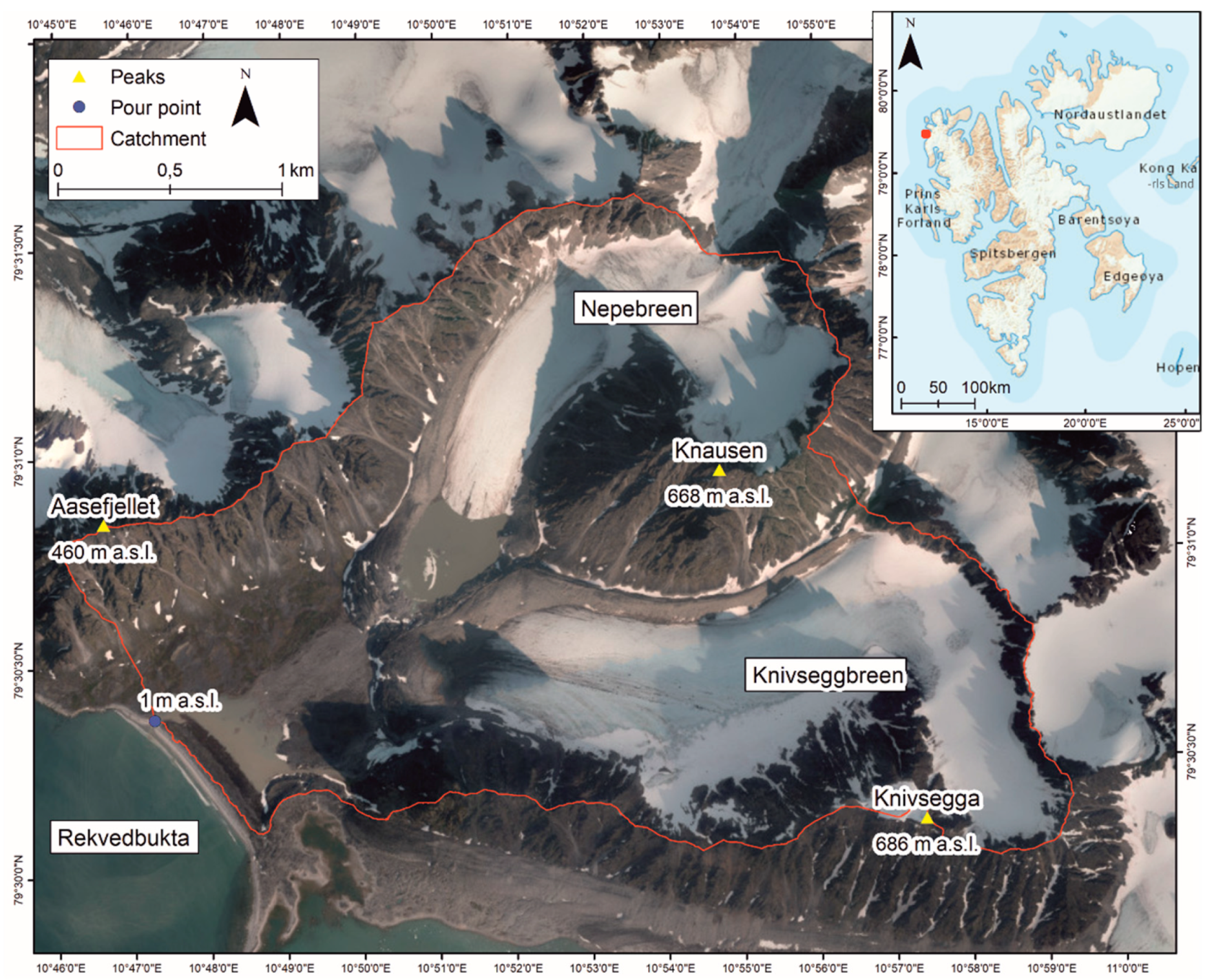
2.1. Study Site

Small catchments are numerous on Svalbard, but they differ in terms of the extent of glaciation, aspect, elevation, river systems, presence of lakes and types of lakes. Rekvedbukta is situated on Albert I Land, ca. 8 km south of Magdalenefjorden. The study area (8 km²) is presented in Figure 2. The bedrock of the catchment is composed of Mesoproterozoic (migmatite and banded gneiss) [28,29] and Ludlow–Pridoli (granitoid rocks) age Smeerenbugfjorden Complex [29]. In the lower parts of the catchment, the bedrock is covered with unconsolidated Holocene materials: moraines, glaci-fluvial and marine deposits [29]. A thrust fault line cuts through the beach [29]. In the central part of the valley, a flattened fluvial area is located with mixed glaci-fluvial material. The beach is composed of moraine (the SE part) and marine (the NW part) material. On the southern slopes of Aasefjellet, numerous talus cones stretch over its entire length. Smaller talus cones can be observed on the Knausen and Knivsegga slopes. The upper part of the catchment is covered by glaciers—Nepebreen and Knivseggbreen (nor. breen = glacier)—with their moraines marking the LIA extent. Both glaciers are linked with Gullybreen, which seeps into the Magdalenefjorden. Besides the two glaciers, there are two unnamed glacial lakes in the catchment that are located on the glaciers’ forelands, and a lagoon (Rekvedtjørna) is located right behind the coastal barrier. The glacial lakes are connected to the lagoon by streams. The foothills of the Aasefjellet slope are covered with vegetation.

2.2. Detection of Glacier, Catchment and Coastal Changes

To properly analyse the changes that have taken place along the Rekvedbukta coastline, we used a range of available remote sensing data. It is important to note that our analysis also included the forelands of the Nepebreen and Knivseggbreen, as well as the runoff zone of the rivers draining these glaciers.

The Svalbard archipelago has, due to its long tradition of research, received numerous environmental and, above all, remote sensing studies [31,32,33,34]. These range from the available, archival topographic maps from the first scientific expeditions to high-resolution satellite images from the last decade. In order to observe the evolution of the coastline in our study area in more detail, we selected a number of aerial and satellite images that we used directly in our analysis (

Table A1. Index of used satellite images for glacial and lake inventory.

Remote Image Date	Source of Remote Sensing Data	Resolution [m]	Vectorisation Scale
21 September 2022	Planet Explorer	3	1:1000
26 August 2022	Planet Explorer	3	1:3000
22 August 2022	Sentinel-2	10	1:1000
21 August 2022	Sentinel 2	10	1:1000
16 August 2022	Planet Explorer	3	1:1000
11 August 2022	Planet Explorer	3	1:1000
1 August 2022	Sentinel-2	10	1:1000
18 July 2022	Planet Explorer	3	1:1250
16 July 2022	Planet Explorer	3	1:1250
5 July 2022	Sentinel-2	10	1:1000
25 June 2022	Sentinel-2	10	1:1000
7 September 2021	Planet Explorer	3	1:1250
2 September 2021	Sentinel-2	10	1:1000
31 August 2021	Planet Explorer	3	1:1250
14 August 2021	Sentinel-2	10	1:1000
3 August 2021	Planet Explorer	3	1:1250
30 July 2021	Planet Explorer	3	1:800
22 July 2021	Planet Explorer	3	1:1250
3 July 2021	Sentinel-2	10	1:3000
25 August 2020	Sentinel-2	10	1:1000
6 August 2020	Planet Explorer	3	1:1250
27 July 2020	Sentinel-2	10	1:1000
1 July 2020	Planet Explorer	3	1:6000
17 September 2019	Planet Explorer	3	1:3000
16 September 2019	Sentinel-2	10	1:1000
6 August 2019	Planet Explorer	3	1:4000
28 July 2019	Planet Explorer	3	1:3000
27 July 2019	Sentinel-2	10	1:1000
18 September 2018	Sentinel-2	10	1:1000
17 August 2018	Sentinel-2	10	1:1000
6 July 2018	Sentinel-2	10	1:4000
10 September 2017	Planet Explorer	3	1:2000
11 August 2017	Planet Explorer	3	1:2000
10 July 2017	Landsat 8	30	1:10,000
1 July 2017	Landsat 8	30	1:10,000
17 September 2015	Landsat 8	30	1:10,000
5 July 2015	Landsat 8	30	1:10,000
10 September 2014	Landsat 8	30	1:10,000
28 July 2014	Landsat 8	30	1:10,000
10 September 2013	Landsat 8	30	1:10,000
30 August 2013	Landsat 8	30	1:10,000
17 August 2011	Landsat 7	30	1:10,000
23 August 2010	Landsat 7	30	1:10,000
26 June 2009	Landsat 7	30	1:10,000
30 June 2008	Landsat 7	30	1:10,000
6 September 2006	Landsat 5	30	1:10,000
9 August 2006	Landsat 5	30	1:10,000
22 June 2004	Landsat 7	30	1:10,000
30 June 2002	Landsat 7	30	1:10,000
10 July 1999	Landsat 7	30	1:10,000
26 August 1998	Landsat 5	30	1:10,000
2 August 1995	Landsat 5	30	1:10,000
12 July 1995	Landsat 5	30	1:10,000
16 August 1993	Landsat 5	30	1:10,000
27 August 1992	Landsat 5	30	1:10,000
31 July 1989	Landsat 5	30	1:10,000
31 August 1988	Landsat 5	30	1:10,000
31 August 1985	Landsat 5	30	1:10,000
1936	[39]	20	1:8000

). The oldest data are from an aerial campaign taken in 1936 by the Norwegian Polar Institute, while the most recent data are from the Planet and Sentinel satellites. For the 1936 aerial photographs, we additionally used the orthophotomap [34]. In addition, we also used data from multiple Landsat satellite missions. All data were appropriately filtered and only scenes with no or low cloud cover were selected. The resolution of the images themselves was good enough to allow a comparative analysis of coastal changes, glacier forelands, as well as of the glaciers themselves. Given the variability in the resolution of the different data sources, we also carried out error propagation analyses to indicate the magnitude of the possible error made during the analysis of the individual remote sensing data. The aspect map was created in ArcMap 10.7.

To demonstrate the changes in the selected small catchment areas over the past decades, we used Geographical Information Systems (GIS) tools and analyses. For this purpose, glaciers, glacial lakes, lagoons and coastlines were vectorised (manually) and measured on the above-mentioned remote sensing images (on which cloud cover and shadows caused no problems for vectorisation) in ArcMap 10.7. For the most recent data, characterised by the best quality (from 3 to 10 m resolution), the rate of shoreline change was calculated using the Digital Shoreline Analysis System (DSAS) available in ArcMap as an add-in. DSAS bases its operation on input data, which are the baseline and shorelines stored in the geodatabase as feature classes [35]. The baseline was generated at a distance of 20 m from the shorelines and was 1671 m long, covering almost the entire barrier coast from the tip of the spit system in the south and the tidal inlet to the lagoon in the north (Figure 1). The shorelines were vectorised, and the corresponding dates were added to the attribute table. In addition, decadal shoreline changes were also calculated with DSAS using remote sensing images from 1936, 1985, 1990, 1999, 2011, 2015, 2020 and 2022. However, the resolution of the available images from the selected years varied from 3 m to 30 m. A higher level of uncertainty in the data was considered, which can be determined by DSAS. The level of uncertainty ranged from 3–15 m depending on the resolution of the image: the worse the resolution, the greater the uncertainty. For this study, the barrier coast blocking the lagoon system was divided into 84 transects of 20 m length. The maximum search distance from the baseline was set to 200 m, which was then clipped to the maximum shoreline extent. Shoreline change statistics were then calculated for the generated transects with a confidence level of 95%. DSAS allowed us to calculate three different parameters characterising shoreline shifts over the 1936–2022 period: [35,36,37,38] End Point Rate (EPR)—the distance between the youngest and oldest shoreline, divided by the time passed between the youngest and oldest shoreline; Shoreline Change Envelope (SCE)—the distance between the furthest and closest shoreline from the baseline, for each transect; Net Shoreline Movement (NSM)—the distance between the youngest and oldest shoreline [35,36,37,38].

Using ArcScene 10.7, a 3D catchment model (for the year 2022) was created to enable us to compare with an aerial oblique photograph from 1936 [39].

We used the Normalised Difference Vegetation Index (NDVI) for two purposes: firstly, to show how the surface area of the vegetation has changed since the 1970s and secondly, how the GLOF event affected the NDVI values. The NDVI was calculated in ArcMap 10. 6. 1 with the standard formula [40]:

NDVI = (NIR − RED)/(NIR + RED)

The following bands were used for the following dates: 1976 and 1980 bands 6 and 7 [41], for 1990, 2000 and 2011 bands 3 and 4 [42,43] and for 2020 bands 8 and 4 [43]. Parts of the used scenes covered with shadows or clouds were excluded from the analysis. For the NDVI GLOF analysis, we used Sentinel-2 data [44] with a 2 × 2 m resolution.

The second index we used in our work was the Normalised Difference Water Index (NDWI). The purpose of the use of this index was to find the areas covered by water. Based on this index, we were able to determine the extent of surface water (in this case, glacial lakes and lagoon), as well as to use satellite images in which the Earth’s surface was obscured by partial cloud cover, preventing the adequate interpretation of the scenes in visible light (RGB) spectra [45]. NDWI was calculated in ArcMap 10.8 using the formula [45]:

NDWI = (GREEN − NIR)/(GREEN + NIR)

3. Results

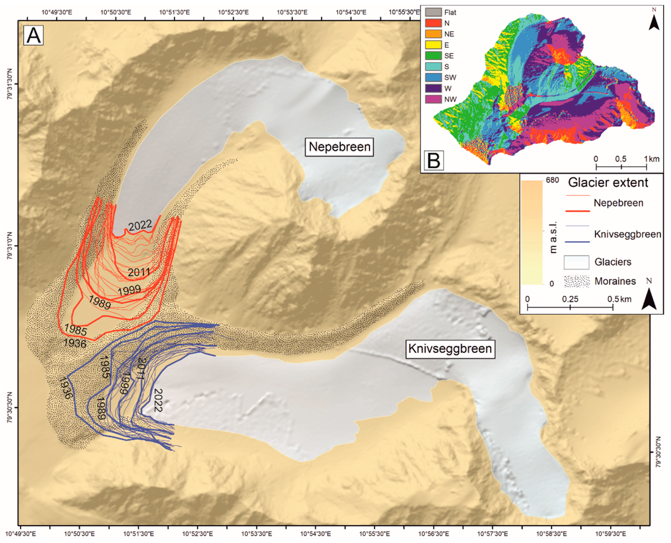
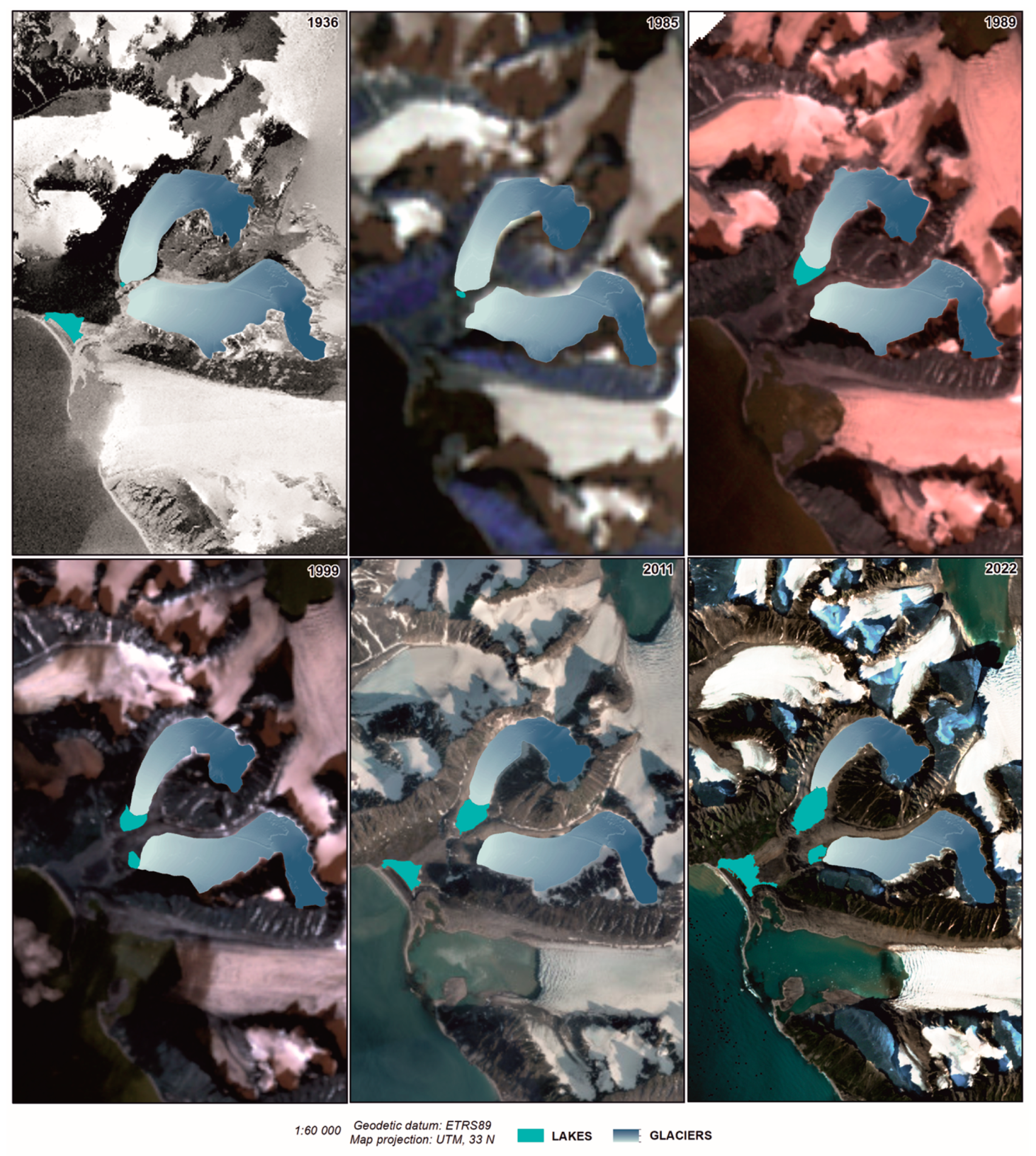
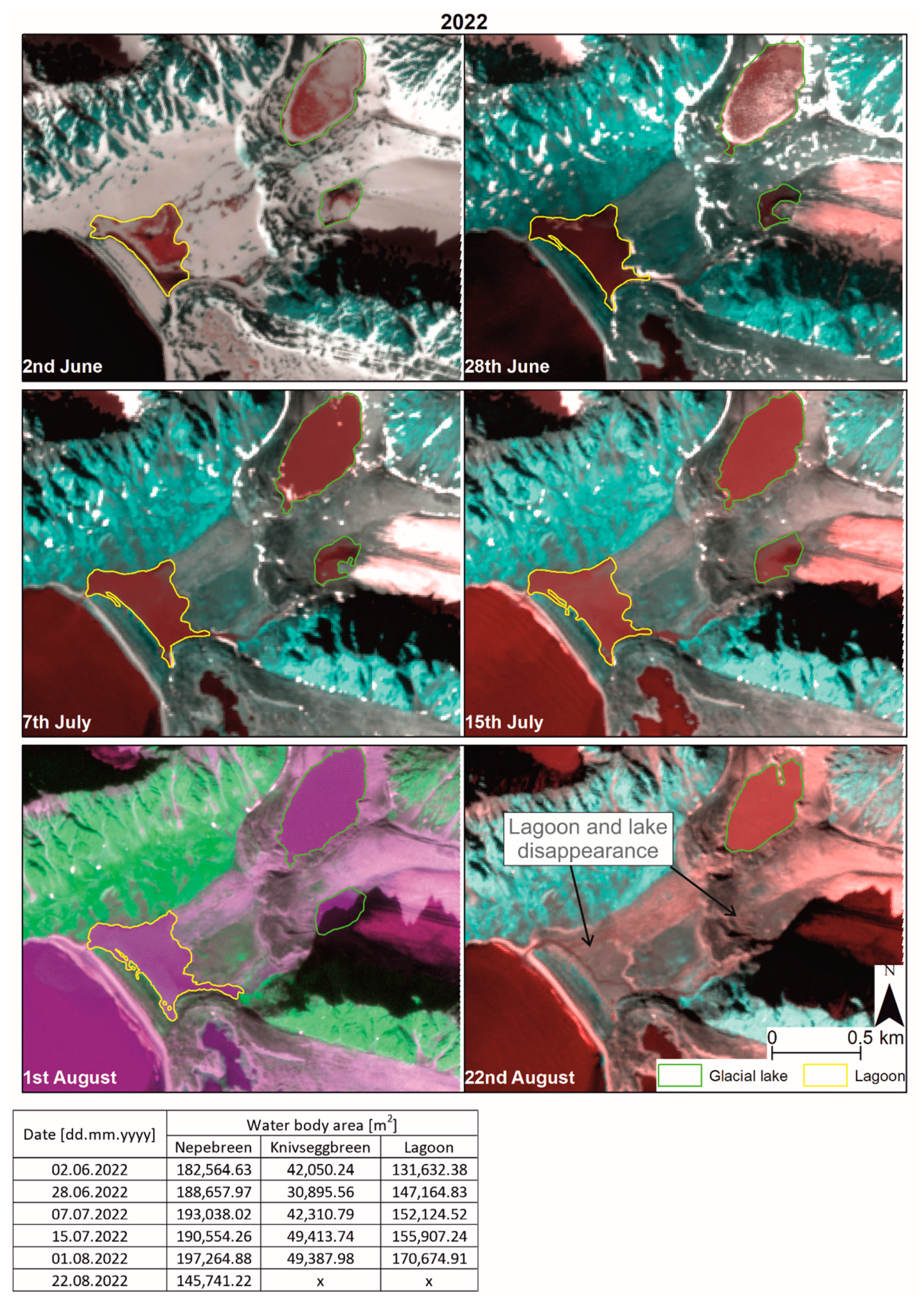
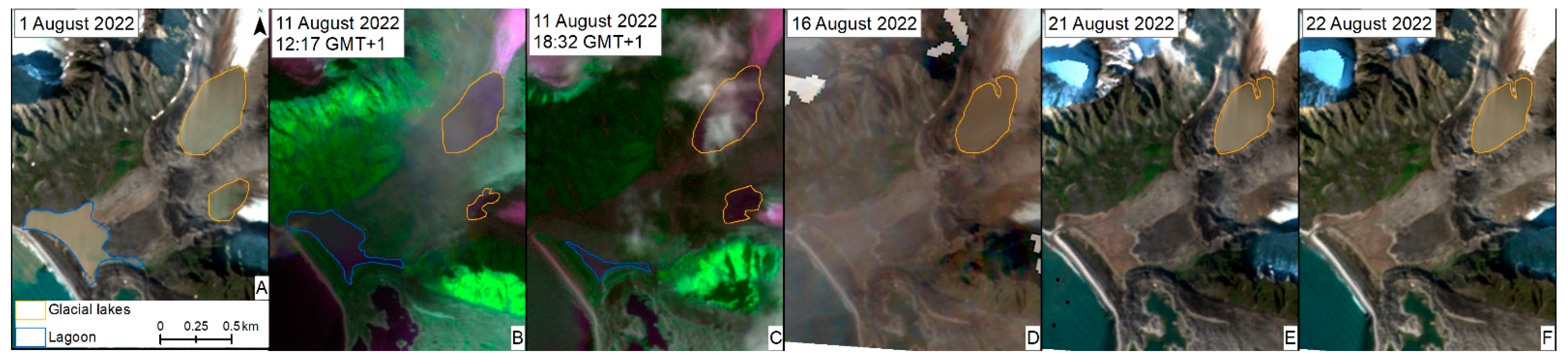
3.1. Deglaciation and GLOF Events

Deglaciation of the analysed area is one of the most important processes for the changing landscape. Given that the oldest material for our analysis is an aerial image from 1936, the glaciers considered in our study were already in the deglaciation phase after the termination of the LIA. According to all the different authors, the LIA ended around 20–30 years before 1936 which, instead, is part of the warm 1930s. The furthest extent of the glaciers during the LIA can therefore be directly related to the position of the end-moraines, which at some point began to bound each other, forming a medial moraine separating Nepebreen and Knivseggbreen (Figure 3). We therefore analysed a number of satellite and aerial photographs to show the deglaciation process of both glaciers. In 1936, both glaciers were still in direct contact with the end-moraines and since then we have only observed their retreat.

We had to take into account the varying resolution of the data used, so we distinguished the limits of the glacier’s extent at an average frequency of every decade (

Table 1. Nepebreen and Knivseggbreen retreat rate since 1936.

Nepebreen—Aspect: SW			Knivseggbreen—Aspect: W
Date	Mean Difference with Previous Glacier Extent [m]	Average Glacier Retreat Length [m] (Average Annual Velocity [m/y])	Date	Mean Difference with Previous Glacier Extent [m]	Average Glacier Retreat Length [m] (Average Annual Velocity [m/y])
1936	-	391 (−4.55)	1936	-	267 (−3.1)
1985	70		1985	50
1989	83		1989	48
1999	24		1999	46
2011	107		2011	59
2022	112		2022	64

).

Nepebreen, with a southwestern aspect (Figure 3), is characterised by an annual retreat rate of approximately 4.55 m/year, which is faster than the western-facing Knivseggbreen’s retreat rate of 3.1 m/year. In addition to the retreat of the glacier fronts themselves, a localised narrowing of the glaciers is also evident, so that they no longer fill the entire valley, as can be seen, for example, in satellite images from the 20th century (Figure 4).

With the retreating glaciers, a glacial lake appeared within the frontal moraine in 1936 on the foreland of Nepebreen, which has developed steadily since then, and in the summer season of 1999, a glacial lake was also formed on the foreland of Knivseggbreen. The lake at Nepebreen was in direct contact with the glacier until 2022 and filled all the free space within the frontal moraine left by the retreating glacier. The lake at Knivseggbreen was originally an ice-contact lake, too, but had already lost its direct contact with the glacier by the late 1990s. Both lakes are classified as end-moraine glacial lakes. The instability of the moraine in front of Knivseggbreen led to the dam bursting and the glacial lake outflows. The first GLOF event occurred back in 1999. After this event, the lake did not form again until the summer season of 2017, when the lake is visible in the satellite image from the 11th of August, only to drain as a GLOF event, as seen in the September 2017 satellite images. After this event, there were five more GLOF events (2018, 2019, 2020, 2021, 2022), which we were able to record by analysing the satellite images. The last known GLOF event occurred in 2022 (Figure 5).

From the perspective of our work, the most interesting GLOF event appeared to be that of August 2022. Using the available remote sensing data, we narrowed down the moment (day) of the GLOF occurrence as much as the quality of the available data and, above all, the cloud cover allowed (Figure 6). With the aim of using as many images as possible to analyse the GLOF event, we used multispectral scenes (Figure 6B,C). Multispectral scenes allowed us to observe this runoff zone despite the unfavourable partial cloud cover. By modifying the scene display with the near-infrared channel, the area occupied by water could be highlighted. On the 1 August, the area of the glacial lake at Knivseggbreen was approximately 0.05 km²; at the same time, the lagoon area was c.a. 0.17 km² (Figure 5). An important satellite image was taken on the 11 August and shows that the glacial lake at Knivseggbreen has significantly reduced its surface area since the 1st of August (−0.02 km², equal to 33% areal loss), while causing the lagoon to fill with sediments and decrease in area by 12:17 UTC (−0.01 km², 7% loss). At the same time, a small sediment outflow with an area c.a. 0.2 km² is visible. In the image taken at 18:37 UTC on the same day, a very large outflow of sediments (4.8 km²; an increase of 4.5 km² or 1834%) from the lagoon into the bay is observed, as well as its drainage (−0.11 km², −69%). The next available satellite image was taken on the 16th of August, but the cloud cover in the image does not allow for an accurate analysis of the extent of the glacial lakes. Nevertheless, it can be seen that the glacial lake at Knivseggbreen and the lagoon have completely drained, and the bay no longer contains as much sediment as during the GLOF event on the 11th of August. After this event, the first satellite scene, which we were able to analyse in detail due to suitable meteorological conditions (cloud cover lower than 50%), was taken on the 21 August. With it, we can confirm with certainty the complete drainage of the glacial lake and lagoon.

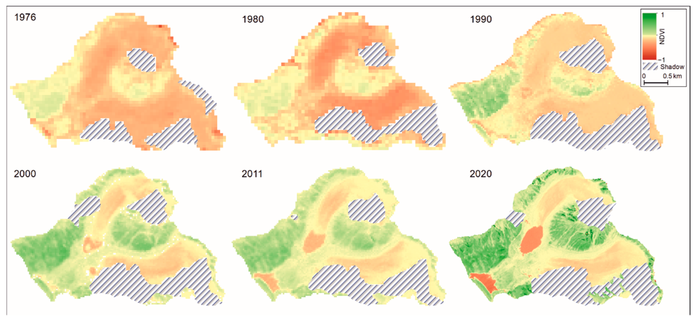
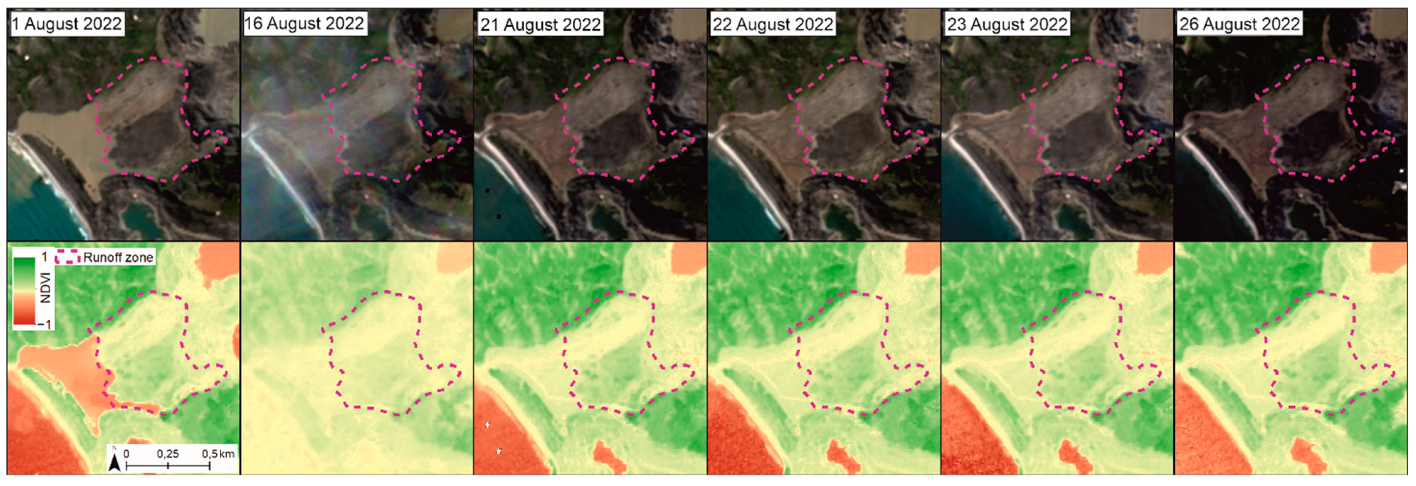
3.2. Environmental Changes in the Glacierised Catchment

The results of climate change on the catchment are easily visible in Figure 3, where the shift in the position of the glacier fronts is clearly seen. The results of the decadal vegetation coverage analysis of the last 45 years showed that the mean spatiotemporal NDVI value increased from −0.17 to 0.12 as well as alongside increases in both the minimum and maximum values (

Table 2. Index and results of satellite images used for NDVI analysis.

Date	Resolution [m]	Satellite	Min Value	Max Value	Mean Value
09 July 1976	60 × 60	Landsat-2	−0.80	0.16	−0.17
22 August 1980	70 × 65	Landsat-2	−0.55	0.13	−0.17
18 August 1990	35 × 35	Landsat-5	−0.35	0.47	−0.06
25 August 2000	30 × 30	Landsat-7	−0.30	0.62	0.08
17 August 2011	30 × 30	Landsat-7	−0.30	0.50	0.06
28 August 2020	2 × 2	Sentinel-2	−1	1	0.12

).

The spatial and temporal location of vegetation is presented in Figure 7. The northern slopes of Knivsegga are often in shadow, precluding an analysis of that area. In the year 2011, little decrease in NDVI values was observed in comparison to the previous year. However, the general spatiotemporal trend showed a positive response of the vegetation to the warming climate within the catchment.

Below we present the influence of the GLOF event, which occurred between the 1 and 16 August 2022, on NDVI in the runoff zone (Figure 8). The 16th of August is the first day when a small cloud cover enabled us to notice environmental changes in the catchment such as lagoon outwash (TC) and a sudden drop in vegetation (NDVI), which occurred over a two-week period. Within the next days (21, 22, 23 and 26 August), greenness reactivation and the usage of old stream channels (visible as very low, reddish, NDVI values) were observed. Further tracing of changes in the runoff zone was impossible due to dense cloud cover and snowfall in September. However, over the following 10 days, after the GLOF event, a rapid positive change in the NDVI values was observed, which suggested low (only sediment coating) GLOF impact in the runoff zone.

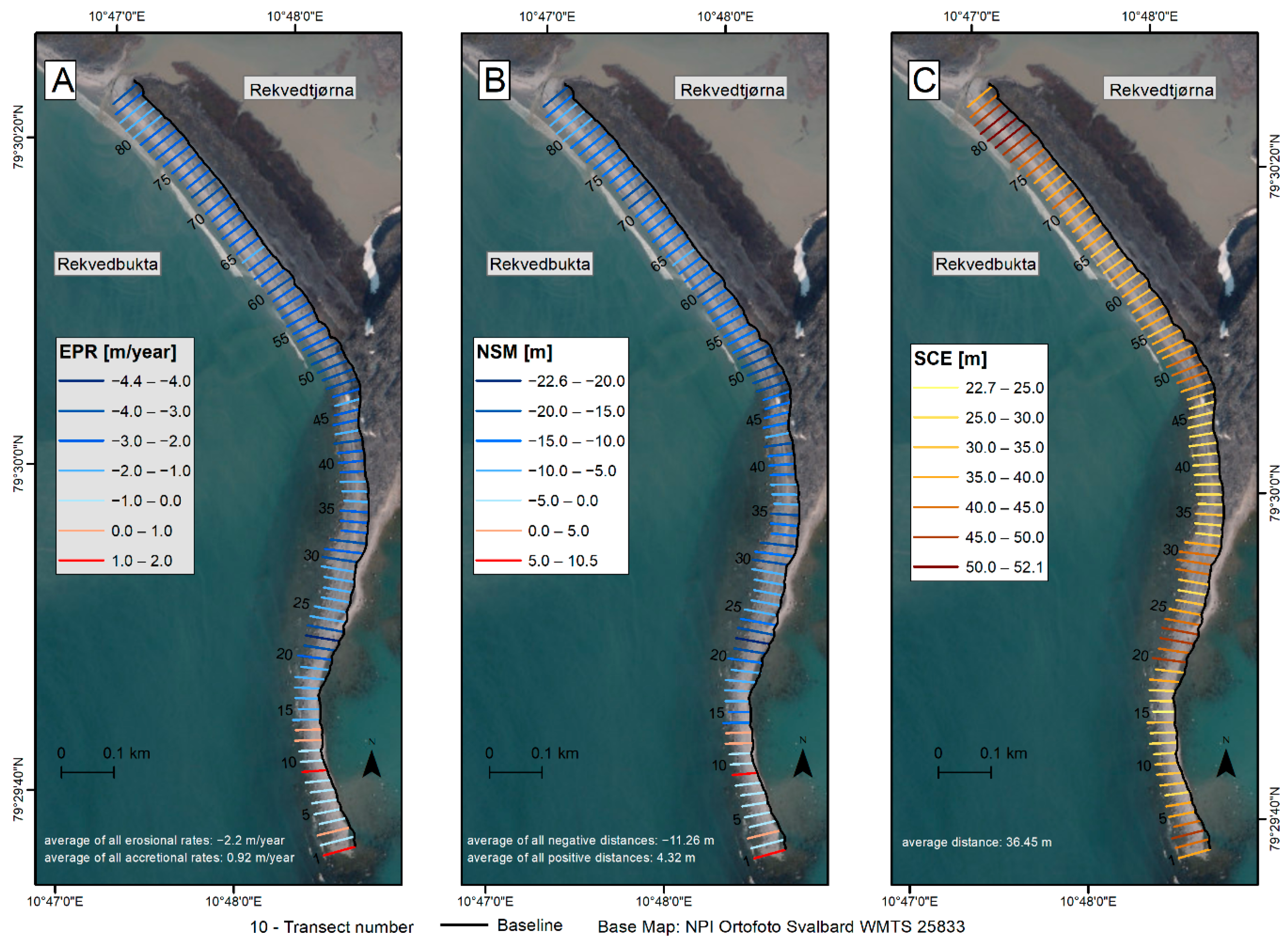
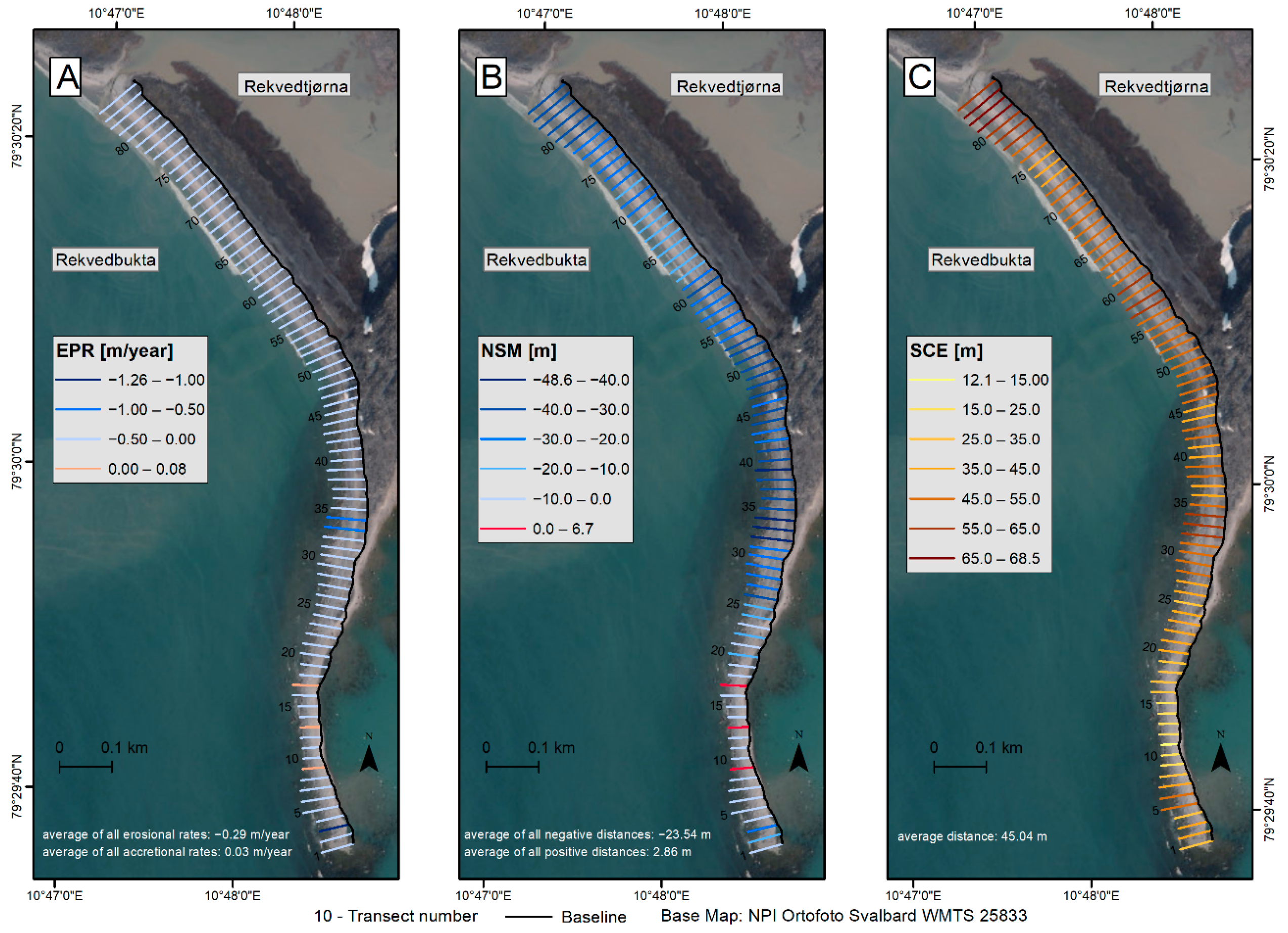
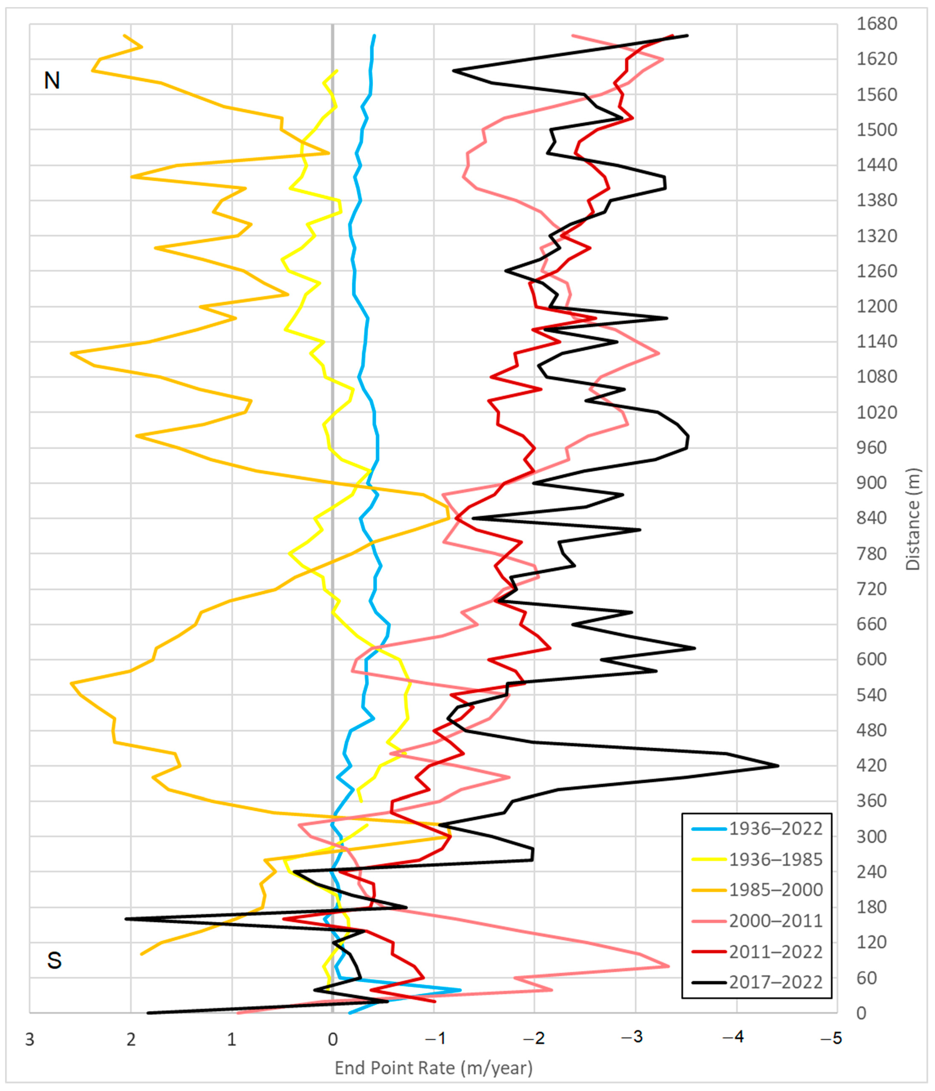
3.3. Shoreline Changes

Analysing the shoreline changes, the EPR (Figure 9A and Figure 10A) showed a significant erosion trend for the data covering the last five years, as well as for the decadal data (1936–2022). The average rate of change for the last five years was −2.2 m/year (Figure 9A) and −0.29 m/year for the decadal data (Figure 10A). The largest EPR erosion (−4.1 m/year) in the last five years was detected in transect 22. In the entire analysed period 1936–2022, the highest mean (EPR) erosion was found in transect 3 (−1.26 m/year). The average of all the accretional rate values of the EPR during 2017–2022 was 0.92 m/year and for the multi-year data was −0.03 m/year. The largest changes in EPR in recent years were seen in the northern part of the coast. For the most part, these were changes of −2 to −4 m/year in the period 2017–2022. In the multi-year period, the northern part continued to show the greatest transformation, but here the changes fluctuated around −0.5 m/year.

For the NSM calculated for the latest years 2017–2022 (Figure 9B), the average distance was −10.33 m, indicating that more erosion than accretion has occurred at the coast over the last five years. Moreover, a negative distance was obtained in 79 transects, with an average of −11.26 m. The largest negative distance was recorded for transect 22: −22.55 m. It is noticeable that the more eroded section of the coast is to the north of this transect. A positive distance was only shown for five transects, with an average offset of 4.32 m. The largest positive distance was shown for transect 9: 10.47 m, which is located in the southern part of the coastline. For the decadal data (Figure 10B), the average NSM was −22.6 m, and the distance was negative in 81 transects. For the same data, the largest negative NSM was calculated for transect 4 (−48.57 m). The largest positive distance was calculated for transect 9 (6.69 m), the same as for 2017–2022. The average positive distance for 1936–2022 was 2.86 m.

The average distance for the SCE analysis between 2017–2022 was 36.45 m (Figure 9C). The largest change occurred in transect 80 where there was a 52.14 m difference between the nearest and the furthest shoreline from the baseline. In this case, the shorelines were the closest on the 21st of September 2022 and the furthest on the 1st of July 2020. This means that more than 50 m of coastline eroded between these two years. The smallest SCE value was shown for transect 15 and reached 22.72 m. In this case, the extreme shorelines were also from 2020 and 2022 and the initial (southern) and central parts of the coast changed less than the final (northern) part of the coast (near to the inlet), where changes mostly reached more than 40 m for each transect. The SCE for the data from 1936–2022 averaged 45.04 m (Figure 10C). The largest displacement during this period was found for transect 82, with a value of 68.46 m (similar to the 2017–2022 data). This displacement was observed in the data from 2022 (the closest shoreline) and 2000 (the furthest shoreline). This is mainly related to the lack of an inlet in the 2000s, when the lagoon lake had no direct connection to the sea. Transect 11 showed the smallest distance of 12.18 m, and this change referred to the same extreme shorelines as above (2000 the furthest and 2022 the closest). When considering multi-year changes, the smallest changes were mainly at the beginning of the coast and the largest, as in the case of 2017–2022, in the final (northern) part near the inlet.

The erosion rate has been increasing since 2000 (Figure 11). We observed that in 2000–2022, the northern part of the coast was eroding at quicker rate than the southern part by around 1 m/year. Between 1985 and 2000, a positive seaward shift of the coastline was observed, indicating accumulation along the entire coastline with the exception of the area from transect 14–17 and 39–45. We relate this phenomenon to the increased delivery of glacial sediments to Rekvedbukta, which were used to develop the barrier, as highlighted by the fact that it has grown in length by 92 m compared to 1936. The presence of water in the lagoon since the early 2000s may have influenced the slowing down of sediment release into Rekvedbukta. In addition, it was noted that eroded material, mainly from the northern part of the coast, was partially deposited in the southern part of the coast, overbuilding the scythe by more than 70 m in length.

4. Discussion

4.1. Glacial Geohazard Influence on Svalbard Coastal Systems

In the last several years, most of the Svalbard coastal change studies concentrated on the investigations of multidecadal shoreline changes associated with the pulses of sediments released from retreating glaciers [17,31,47,48,49,50,51,52]. Most of these gravel-dominated or mixed sand–gravel barrier coasts prograded in periods of uninterrupted glaciofluvial sediment supply (up to 3–5 m/year) and retreated (ca. 1 m/year) in times when glacier rivers overcame channel shifts, resulting in either a change of the river mouth location or the deposition of sediment load along the extended valley. In contrast, on the coast we analysed, the average EPR for the period 1936–2022 was −0.28 ± 0.06 m/year, which we interpret as a predominance of erosion. Moreover, for the last few years, the erosion level was as high as −2.2 m/year. We can deduce that the supply of sediment from the glaciers was, in this case, slowed down by the formation of glacial lakes, which served as a reservoir to temporarily store sediments [53] that could overbuild the coast. The spit in the southern part of the coast is protected from the sea by rocks and is therefore not subject to the same erosion as the northern side, which has no natural barrier. This would explain why the coast is eroded with different intensity. In addition, together with coastal currents, material eroded in the northern part could have been used to overbuild the spit in the southern part. A similar situation was demonstrated by Strzelecki (et al., 2018) [52] at Petuniabukta, where eroded material from the Ferdinand Fan deltas was used to overbuild modern barriers.

More recently, Strzelecki et al. [54] described the diversity of coastal landforms formed after the exposure of new fjord shorelines from the retreat of tide-water glaciers in Brepollen (southern Spitsbergen). In the bay formed in the last 80 years, the juvenile coastal landscape evolved from the reworking of glacial forms and sediments, by waves and tides, with a less significant role played by fluvial processes. Along almost 90 km of new coasts exposed over the last century, the whole mosaic of landforms from rocky cliffs, through deltas, barrier islands, and pocket beaches up to lagoons were mapped. Here it is crucial to mention that coastal lagoon systems are one of the most sensitive environments to the ongoing global changes as they accumulate the effects of environmental changes occurring on both the land and the sea [31,55]. Globally, the stability of lagoons and associated barriers are controlled by the frequency and magnitude of storms approaching the coasts, access to sediment supplies and resilience to sea-level rise [31,56,57,58]. It is noteworthy that, up until now, studies on Svalbard lagoon coast morphodynamics have been almost entirely neglected. An interesting example of the interplay between a retreat tidewater glacier exposing the coast to enhanced erosion and the stability of the lagoon was presented by Ziaja et al. [59]. At the turn of the 19th and 20th centuries, the massive tongue of Hambergbreen extended a few kilometres into the Barents Sea and formed an ice-cliffed bay where Davislaguna developed. Since the termination of the LIA, the glacier front not only retreated over 10 km and formed a new bay—Hambergbukta—but also exposed a section of the coast to the direct operation of storm waves. As a consequence, the coastal barrier forming Davislaguna was breached and later on fully eroded, leading to the disappearance of the lagoon. After breaching the barrier, the shoreline shifted landward over 450 m, which to date is the largest shoreline change detected in Svalbard during the last century.

In our study, however, we managed to capture the previously undescribed processes of extreme lagoon drainage triggered by a glacial outburst flood event. The most recent GLOF that drained the Knivseggbreen glacial lake in August 2022 not only flooded the Rekvedtjørna lagoon but most probably closed the lagoon inlet and filled the lagoon basin with glaciogenic sediments eroded from the glacier foreland and valley. This may explain why we could not detect water in the lagoon after the GLOF event. We suppose that with continued glacier retreat and the associated glacioisostatic uplift of the land, this process may lead to the complete cut-off of the lagoon from the sea and a lack of marine water infill. Svalbard lagoons form through the development of barriers supplied with sediments from predominately glacial catchments. Lagoons exist until the tidal inlet is open and allows sea waters to enter the lagoon basin. With glacioisostatic uplift, the supply of water through the inlet is reduced, which can lead to a complete lack of connection to the sea and the creation of a lagoon lake [54,55].

4.2. GLOFs As Landscape Shaping Processes

A rapid development of glacial lakes has been observed worldwide since the 1990s [21], with the Svalbard archipelago following this trend [22]. As such, we increasingly have to consider the heightened threat of glacial lake outburst floods [60]. The glacial lake on the Nepebreen foreland confirms this accelerated global development of glacial lakes since the 1990s, which we can systematically analyse with the timeline we have presented. The seasonal changes of glacial lakes also stand out here, indicating that they mostly reach their surface maximum in late July/early August, when lake drainage takes place [26]. Drainage in end-moraine-dammed lakes mostly occurs due to the instability of the moraines themselves [61] or due to water overtopping the dam [62]. In the case of the two glacial lakes analysed, the dam has broken, and an outlet has deepened, through which the lakes are systematically drained every season, either fully or partially. Conditions at the Nepebreen forefield are favourable for water retention and the lake continuously maintains a relatively large surface area. There are a few factors that favour the formation of glacial lakes, or to be more accurate in this case, proglacial lakes. It should be noted that the morphology of the area is related to historical glacial activity. The U-shaped valleys that were formed are now being exposed due to the recession of the glaciers and are crucial for the possible formation of proglacial lakes. The favourable conditions are therefore above all a wide and low-sloped valley and the formation of a high frontal moraine [63]. The importance of glacial valley overdeepenings due to glacial erosion, which directly affect the potential volume of an end-moraine glacial lake, must be mentioned [63]. The DEM indicates that a bigger overdeepening valley was formed by Knivseggbreen (the difference between the top of the dam and the surface of the glacial lake is about 7 m greater than on Nepebreen). However, the higher rate of retreat of the Nepebreen allowed the development of the glacial lake. In the case of Knivseggbreen, the glacial lake had considerably less space to expand, which is why water piled up right next to the frontal moraine, resulting in a breach of the dam structure and the occurrence of five GLOF events. Seasonal runoffs of glacial lakes are associated with the reaching of a certain level of maximum instability due to ice melt, rainfall or direct glacial activity [64]. Given the varying magnitude of the environmental impact of glacial floods, the event we described was only of a regional scale [23,65,66]. The glacial floods led to a significant remodelling of the foreland by changing the layout of the channel network through which the water flows, by eroding (or at least covering) the vegetation with sediment, and by significant sediment deposition into the lagoon from which the sediments were then pushed out and deposited in the bay [53].

4.3. Landscape Changes in Small Catchments

Since the end of the LIA, the catchment has experienced major change, as can be seen in Figure 10. Small glaciers, often located in small catchments, experience a similar mass loss to larger ice masses [67]. Svalbard glaciers’ Equilibrium Line Altitude (ELA) was at 440 ± 80 m a.s.l. in 2020 [68], thus most parts of Nepebreen and Knivseggbreen are below this line. Nevertheless, the cirque areas of the glaciers are above the ELA, which may help in their resilience to climate warming.

Sediment release is faster and more intense the smaller the catchment is; moreover, the availability of sediment is the highest in the first 200 years after deglaciation with the highest rates occurring right after deglaciation, before declining over time [69]. Thus, we can expect to see high rates of sediment release in the catchment. In the satellite images of Rekvedbukta it is possible to observe the sediment yield, as it is related to the retreating glaciers, as well as to the lakes that act as a buffer before sediments reach the sea.

The lagoon is clearly visible in the 1936 image (Figure 12). Due to the lack of data, we do not know what happened between 1936 and 1985, but the lagoon is not filled with water in the years 1985–2000. We can suppose that an event took place that led to the lagoon disappearance. Even though we can observe the presence of glacial lakes in the 1980s and 1990s, the lagoon was not filled with water. We can suppose that the Svalbard uplift enhanced the water retention in the lagoon. The mean rate of uplift in Ny-Ålesund, which is the closest uplift control point to our study, in the years 2000–2013 was 7.94 ± 0.21 mm/year [70]. Therefore, we can assume that in 1936 the lagoon was filled with sea water and is currently mostly filled by meltwater (glacial meltwater, permafrost thawing water, and precipitation) thanks to the ongoing inlet uplift. In the 2009 orthophotomap [30], numerous pieces of driftwood can be found above the northern bank of the lagoon, which proves the occurrence of intensive storms or tsunami waves in the past, or alternatively higher lagoon water levels nowadays marked with logs of wood. The wood is located at 4 m a.s.l. and clearly shows previous water extent (Figure A1). The wood may also represent a contemporary water extent during heavy storm floodings, which occur a few times every year. However, more data including local wave height measurements are crucial to confirm such an extreme water level.

The greater NDVI values are related to higher phytomass in the shrub communities [71], thus we can conclude that vegetation within the catchment is becoming denser and more widely distributed, corresponding with the Arctic greening concept [42,72,73]. The authors of [40] indicate a 0.50 value as the maximum NDVI in the Arctic, which makes the maximum values from the years 2000 and 2020 uncertain. Uncertainty can be related to satellite data problems or the presence of non-eliminated falsified raster cells.

5. Conclusions

The effects of climate change such as glacier retreat, glacial lake formation, the degradation of dead ice-moraine belts, glacial outburst floods, lagoon vanishing and filling with glacial sediments, coastal zone changes (progradation and/or erosion of barriers and spits), and the development of spit and vegetation advances are well pronounced in small catchments. Since the end of the LIA, Svalbard, among the other Arctic regions, has been experiencing severe environmental shifts which have led to the intensification of land shaping processes. Based on our research, the shoreline at Rekvedbukta has retreated landward by an average of 45.04 m over the last century, and the rate of change (in this case due to erosion) averaged 0.33 m/year. The Nepebreen and Knivseggbreen rates of areal retreat were found to be 4.55 m/year and 3.1 m/year, respectively. Frontal retreat averaged 391 m and 267 m in the years 1936‒2022. Glacial retreat allowed glacial lakes to form, giving rise to the possibility of GLOFs, which have occurred six times at the Knivseggbreen in recent years. At this local scale, climate warming resulted in intense sediment release into the sea as well as the GLOF event (August 2022), which further influenced the catchment’s vegetation, drainage system, and most of the lagoon and coast. After the flood, the lagoon remained dry. The spatiotemporal analysis of vegetation showed that, in the last 45 years, vegetation has expanded and mean phytomass values (having direct impact on NDVI) have risen from −0.17 to 0.12.

Our research shows how rapidly (within a two-week period) major hydrological changes can occur in a small coastal catchment, proving the instability of high Arctic environments in a warming climate.

References

1. Rantanen, M.; Karpechko, A.Y.; Lipponen, A.; Nordling, K.; Hyvärinen, O.; Ruosteenoja, K.; Vihma, T.; Laaksonen, A. The Arctic Has Warmed Nearly Four Times Faster than the Globe since 1979. Commun. Earth Environ. 2022, 3, 168. [Google Scholar] [CrossRef]
2. Overland, J.E.; Wang, M.; Walsh, J.E.; Stroeve, J.C. Future Arctic Climate Changes: Adaptation and Mitigation Time Scales. Earths Future 2014, 2, 68–74. [Google Scholar] [CrossRef]
3. Biskaborn, B.K.; Smith, S.L.; Noetzli, J.; Matthes, H.; Vieira, G.; Streletskiy, D.A.; Schoeneich, P.; Romanovsky, V.E.; Lewkowicz, A.G.; Abramov, A.; et al. Permafrost Is Warming at a Global Scale. Nat. Commun. 2019, 10, 264. [Google Scholar] [CrossRef] [PubMed] [Green Version]
4. Allaart, L.; Schomacker, A.; Håkansson, L.M.; Farnsworth, W.R.; Brynjólfsson, S.; Grumstad, A.; Kjellman, S.E. Geomorphology and Surficial Geology of the Femmilsjøen Area, Northern Spitsbergen. Geomorphology 2021, 382, 107693. [Google Scholar] [CrossRef]
5. Osuch, M.; Wawrzyniak, T.; Nawrot, A. Diagnosis of the Hydrology of a Small Arctic Permafrost Catchment Using HBV Conceptual Rainfall-Runoff Model. Hydrol. Res. 2019, 50, 459–478. [Google Scholar] [CrossRef] [Green Version]
6. Nielsen, D.M.; Pieper, P.; Barkhordarian, A.; Overduin, P.; Ilyina, T.; Brovkin, V.; Baehr, J.; Dobrynin, M. Increase in Arctic Coastal Erosion and Its Sensitivity to Warming in the Twenty-First Century. Nat. Clim. Chang. 2022, 12, 263–270. [Google Scholar] [CrossRef]
7. Fritz, M.; Vonk, J.E.; Lantuit, H. Collapsing Arctic Coastlines. Nat. Clim. Chang. 2017, 7, 6–7. [Google Scholar] [CrossRef] [Green Version]
8. Screen, J.A. Arctic Amplification Decreases Temperature Variance in Northern Mid- to High-Latitudes. Nat. Clim. Chang. 2014, 4, 577–582. [Google Scholar] [CrossRef] [Green Version]
9. Moon, T.A.; Overeem, I.; Druckenmiller, M.; Holland, M.; Huntington, H.; Kling, G.; Lovecraft, A.L.; Miller, G.; Scambos, T.; Schädel, C.; et al. The Expanding Footprint of Rapid Arctic Change. Earths Future 2019, 7, 212–218. [Google Scholar] [CrossRef] [Green Version]
10. Barnhart, K.R.; Overeem, I.; Anderson, R.S. The Effect of Changing Sea Ice on the Physical Vulnerability of Arctic Coasts. Cryosphere 2014, 8, 1777–1799. [Google Scholar] [CrossRef]
11. Young, I.R.; Zieger, S.; Babanin, A.V. Global Trends in Wind Speedand Wave Height. Science (1979) 2011, 332, 448–451. [Google Scholar] [CrossRef]
12. Lantuit, H.; Overduin, P.P.; Couture, N.; Wetterich, S.; Aré, F.; Atkinson, D.; Brown, J.; Cherkashov, G.; Drozdov, D.; Donald Forbes, L.; et al. The Arctic Coastal Dynamics Database: A New Classification Scheme and Statistics on Arctic Permafrost Coastlines. Estuaries Coasts 2012, 35, 383–400. [Google Scholar] [CrossRef] [Green Version]
13. Overduin, P.P.; Strzelecki, M.C.; Grigoriev, M.N.; Couture, N.; Lantuit, H.; St-Hilaire-Gravel, D.; Günther, F.; Wetterich, S. Coastal Changes in the Arctic. Geol. Soc. Spec. Publ. 2014, 388, 103–129. [Google Scholar] [CrossRef]
14. Irrgang, A.M.; Bendixen, M.; Farquharson, L.M.; Baranskaya, A.V.; Erikson, L.H.; Gibbs, A.E.; Ogorodov, S.A.; Overduin, P.P.; Lantuit, H.; Grigoriev, M.N.; et al. Drivers, Dynamics and Impacts of Changing Arctic Coasts. Nat. Rev. Earth Environ. 2022, 3, 39–54. [Google Scholar] [CrossRef]
15. Kasprzak, M.; Strzelecki, M.C.; Traczyk, A.; Kondracka, M.; Lim, M.; Migała, K. On the Potential for a Bottom Active Layer below Coastal Permafrost: The Impact of Seawater on Permafrost Degradation Imaged by Electrical Resistivity Tomography (Hornsund, SW Spitsbergen). Geomorphology 2016, 293, 347–359. [Google Scholar] [CrossRef] [Green Version]
16. Bendixen, M.; Lønsmann Iversen, L.; Anker Bjørk, A.; Elberling, B.; Westergaard-Nielsen, A.; Overeem, I.; Barnhart, K.R.; Abbas Khan, S.; Box, J.E.; Abermann, J.; et al. Delta Progradation in Greenland Driven by Increasing Glacial Mass Loss. Nature 2017, 550, 101–104. [Google Scholar] [CrossRef]
17. Bourriquen, M.; Mercier, D.; Baltzer, A.; Fournier, J.; Costa, S.; Roussel, E. Paraglacial Coasts Responses to Glacier Retreat and Associated Shifts in River Floodplains over Decadal Timescales (1966–2016), Kongsfjorden, Svalbard. Land Degrad. Dev. 2018, 29, 4173–4185. [Google Scholar] [CrossRef]
18. Strzelecki, M.C.; Long, A.J.; Lloyd, J.M. Post-Little Ice Age Development of a High Arctic Paraglacial Beach Complex. Permafr. Periglac. Process. 2017, 28, 4–17. [Google Scholar] [CrossRef] [Green Version]
19. Strzelecki, M.C.; Jaskólski, M.W.; Strzelecki, M.C. Arctic Tsunamis Threaten Coastal Landscapes and Communities -Survey of Karrat Isfjord 2017 Tsunami Effects in Nuugaatsiaq, Western Greenland. Nat. Hazards Earth Syst. Sci. 2020, 20, 2521–2534. [Google Scholar] [CrossRef]
20. Jarosz, K.; Zagórski, P.; Moskalik, M.; Lim, M.; Rodzik, J.; Mędrek, K. A New Paraglacial Typology of High Arctic Coastal Systems: Application to Recherchefjorden, Svalbard. Ann. Am. Assoc. Geogr. 2022, 112, 184–205. [Google Scholar] [CrossRef]
21. Shugar, D.H.; Burr, A.; Haritashya, U.K.; Kargel, J.S.; Watson, C.S.; Kennedy, M.C.; Bevington, A.R.; Betts, R.A.; Harrison, S.; Strattman, K. Rapid Worldwide Growth of Glacial Lakes since 1990. Nat. Clim. Chang. 2020, 10, 939–945. [Google Scholar] [CrossRef]
22. Wieczorek, I.; Strzelecki, M.C.; Stachnik, L.; Yde, J.C.; Małecki, J. Inventory and Classification of the Post Little Ice Age Glacial Lakes in Svalbard. Cryosphere Discuss. 2022, preprint. [Google Scholar] [CrossRef]
23. Tomczyk, A.M.; Ewertowski, M.W.; Carrivick, J.L. Geomorphological Impacts of a Glacier Lake Outburst Flood in the High Arctic Zackenberg River, NE Greenland. J. Hydrol. 2020, 591, 125300. [Google Scholar] [CrossRef]
24. Rick, B.; Mcgrath, D.; Armstrong, W.; Mccoy, S.W. Dam type and lake location characterize ice-marginal lake area change in Alaska and NW Canada between 1984 and 2019. Cryosphere 2022, 16, 297–314. [Google Scholar] [CrossRef]
25. How, P.; Messerli, A.; Mätzler, E.; Santoro, M.; Wiesmann, A.; Caduff, R.; Langley, K.; Bojesen, M.H.; Paul, F.; Kääb, A.; et al. Greenland-Wide Inventory of Ice Marginal Lakes Using a Multi-Method Approach. Sci. Rep. 2021, 11, 4481. [Google Scholar] [CrossRef]
26. Dudek, J.; Wieczorek, I.; Suwiński, M.K.; Strzelecki, M. Multidecadal Analysis of Paraglacial Landscape Changes in the Foreland of Gåsbreen—Sørkapp Land, Svalbard. Authorea 2022, preprints. [Google Scholar] [CrossRef]
27. Speetjens, N.J.; Hugelius, G.; Gumbricht, T.; Lantuit, H.; Berghuijs, W.R.; Pika, P.A.; Poste, A.; Vonk, J.E. The Pan-Arctic Catchment Database (ARCADE). Earth Syst. Sci. Data Discuss. in review. 2022. [Google Scholar] [CrossRef]
28. Elvevold, S.; Dallmann, W.; Blomeier, D. Geology of Svalbard; Allen Institute for AI: Seattle, WA, USA, 2007; ISBN 9788276662375. [Google Scholar]
29. Dallmann, W.; Piepjohn, K.; McCann, A.; Sirotkin, A.; Ohta, Y.; Gjelsvik, T. Geological Map of Svalbard 1:100,000, Sheet A5G Magdalenefjorden; SUDOC: Pittsburgh, PA, USA, 2005. [Google Scholar]
30. Norwegian Polar Institute. © Norwegian Polar Institute. Available online: https://www.npolar.no/ (accessed on 18 November 2022).
31. Zagórski, P.; Jarosz, K.; Superson, J. Integrated Assessment of Shoreline Change along the Calypsostranda (Svalbard) from Remote Sensing, Field Survey and GIS. Mar. Geod. 2020, 43, 433–471. [Google Scholar] [CrossRef]
32. Jawak, S.D.; Andersen, B.N.; Pohjola, V.; Godøy, Ø.; Hübner, C.; Jennings, I.; Ignatiuk, D.; Holmén, K.; Sivertsen, A.; Hann, R.; et al. Sios’s Earth Observation (Eo), Remote Sensing (Rs), and Operational Activities in Response to COVID-19. Remote Sens. 2021, 13, 712. [Google Scholar] [CrossRef]
33. Kavan, J. Early Twentieth Century Evolution of Ferdinand Glacier, Svalbard, Based on Historic Photographs and Structure-from-Motion Technique. Geogr. Ann. Ser. A Phys. Geogr. 2020, 102, 57–67. [Google Scholar] [CrossRef]
34. Geyman, E.C.; van Pelt, W.J.J.; Maloof, A.C.; Aas, H.F.; Kohler, J. Historical Glacier Change on Svalbard Predicts Doubling of Mass Loss by 2100. Nature 2022, 601, 374–379. [Google Scholar] [CrossRef] [PubMed]
35. Himmelstoss, E.A.; Henderson, R.E.; Kratzmann, M.G.; Farris, A.S. Digital Shoreline Analysis System (DSAS) Version 5.1 User Guide; Open-File Report 2021-1091; USGS: Reston, VA, USA, 2021. [Google Scholar]
36. Baig, M.R.I.; Ahmad, I.A.; Shahfahad; Tayyab, M.; Rahman, A. Analysis of Shoreline Changes in Vishakhapatnam Coastal Tract of Andhra Pradesh, India: An Application of Digital Shoreline Analysis System (DSAS). Ann. GIS 2020, 26, 361–376. [Google Scholar] [CrossRef]
37. Abdul Maulud, K.N.; Selamat, S.N.; Mohd, F.A.; Md Noor, N.; Wan Mohd Jaafar, W.S.; Kamarudin, M.K.A.; Ariffin, E.H.; Adnan, N.A.; Ahmad, A. Assessment of Shoreline Changes for the Selangor Coast, Malaysia, Using the Digital Shoreline Analysis System Technique. Urban Sci. 2022, 6, 71. [Google Scholar] [CrossRef]
38. Sheeja, P.S.; Ajay Gokul, A.J. Application of Digital Shoreline Analysis System in Coastal Erosion Assessment. Int. J. Eng. Sci. Comput. 2016, 6, 7876–7883. [Google Scholar] [CrossRef]
39. Geyman, E.C.; van Pelt, W.J.J.; Maloof, A.C.; Aas, H.F.; Kohler, J. 1936/1938 DEM of Svalbard [Data Set]; Norwegian Polar Institute: Tromsø, Norway, 2021. [Google Scholar] [CrossRef]
40. Bhatt, U.S.; Walker, D.A.; Raynolds, M.K.; Walsh, J.E.; Bieniek, P.A.; Cai, L.; Comiso, J.C.; Epstein, H.E.; Frost, G.V.; Gersten, R.; et al. Climate Drivers of Arctic Tundra Variability and Change Using an Indicators Framework. Environ. Res. Lett. 2021, 16, 055019. [Google Scholar] [CrossRef]
41. Markham, B.L.; Barker, J.L. Spectral Characterization of the Landsat-4 MSS Sensors. Photogramm Eng Remote Sens. 1983, 49, 811–833. [Google Scholar]
42. Johansen, B.; Tømmervik, H. The Relationship between Phytomass, NDVI and Vegetationcommunities on Svalbard. Int. J. Appl. Earth Obs. Geoinf. 2014, 27, 20–30. [Google Scholar] [CrossRef]
43. USGS. Available online: https://Earthexplorer.Usgs.Gov/ (accessed on 18 November 2022).
44. SentinelHub EOBrowser. Available online: https://www.sentinel-hub.com/explore/eobrowser/ (accessed on 18 November 2022).
45. Li, J.; Meng, Y.; Li, Y.; Cui, Q.; Yang, X.; Tao, C.; Wang, Z.; Li, L.; Zhang, W. Accurate Water Extraction Using Remote Sensing Imagery Based on Normalized Difference Water Index and Unsupervised Deep Learning. J. Hydrol. 2022, 612, 128202. [Google Scholar] [CrossRef]
46. Porter, C.; Howat, I.; Noh, M.-J.; Husby, E.; Khuvis, S.; Danish, E.; Tomko, K.; Gardiner, J.; Negrete, A.; Yadav, B.; et al. ArcticDEM – Strips, Version 4.1. Harvard Dataverse 2022, V1. [Google Scholar] [CrossRef]
47. Mercier, D.; Laffly, D. Actual Paraglacial Progradation of the Coastal Zone in the Kongsfjorden Area, Western Spitsbergen (Svalbard). Geol. Soc. Spec. Publ. 2005, 242, 111–117. [Google Scholar] [CrossRef]
48. Zagórski, P. Shoreline Dynamics of Calypsostranda (NW Wedel Jarlsberg Land, Svalbard)during the Last Century. Pol. Polar Res. 2011, 32, 67–99. [Google Scholar] [CrossRef]
49. Kim, D.; Jo, J.; Nam, S.-I.; Choi, K. Morphodynamic Evolution of Paraglacial Spit Complexes on a Tide-Influenced Arctic Fjord Delta (Dicksonfjorden, Svalbard). Mar. Geol. 2022, 447, 106800. [Google Scholar] [CrossRef]
50. Kavan, J. Post-Little Ice Age Development of Coast in the Locality of Kapp Napier, Central Spitsbergen, Svalbard Archipelago. Mar. Geod. 2020, 43, 234–247. [Google Scholar] [CrossRef]
51. Zagórski, P. The Influence of Glaciers on Transformation of the Coast of NW Part of Wedel Jarlsberg Land (Spitsbergen) in Late Pleistocene and Holocene. Słupskie Pr. Geogr. 2007, 4, 157–169. [Google Scholar]
52. Strzelecki, M.C.; Long, A.J.; Lloyd, J.M.; Małecki, J.; Zagórski, P.; Pawłowski, Ł.; Jaskólski, M. The Role of Rapid Glacier Retreat and Landscape Transformation in Controlling the Post-Little Ice Age Evolution of Paraglacial Coasts in Central Spitsbergen (Billefjorden, Svalbard). Land Degrad. Dev. 2018, 29, 1962–1978. [Google Scholar] [CrossRef] [Green Version]
53. Kavan, J.; Wieczorek, I.; Tallentire, G.D.; Demidionov, M.; Uher, J.; Strzelecki, M.C. Estimating Suspended Sediment Fluxes from the Largest Glacial Lake in Svalbard to Fjord System Using Sentinel-2 Data: Trebrevatnet Case Study. Water 2022, 14, 1840. [Google Scholar] [CrossRef]
54. Strzelecki, M.C.; Szczuciński, W.; Dominiczak, A.; Zagórski, P.; Dudek, J.; Knight, J. New Fjords, New Coasts, New Landscapes: The Geomorphology of Paraglacial Coasts Formed after Recent Glacier Retreat in Brepollen (Hornsund, Southern Svalbard). Earth Surf. Process. Landf. 2020, 45, 1325–1334. [Google Scholar] [CrossRef] [Green Version]
55. Mitchell, S.; Boateng, I.; Couceiro, F. Influence of Flushing and Other Characteristics of Coastal Lagoons Using Data from Ghana. Ocean Coast. Manag. 2017, 143, 26–37. [Google Scholar] [CrossRef] [Green Version]
56. Vermaire, J.C.; Pisaric, M.F.J.; Thienpont, J.R.; Courtney Mustaphi, C.J.; Kokelj, S.V.; Smol, J.P. Arctic Climate Warming and Sea Ice Declines Lead to Increased Storm Surge Activity. Geophys. Res. Lett. 2013, 40, 1386–1390. [Google Scholar] [CrossRef]
57. Jones, B.M.; Arp, C.D.; Jorgenson, M.T.; Hinkel, K.M.; Schmutz, J.A.; Flint, P.L. Increase in the Rate and Uniformity of Coastline Erosion in Arctic Alaska. Geophys. Res. Lett. 2009, 36, L03503. [Google Scholar] [CrossRef]
58. Carrasco, A.R.; Ferreira, O.; Roelvink, D. Coastal Lagoons and Rising Sea Level: A Review. Earth Sci. Rev. 2016, 154, 356–368. [Google Scholar] [CrossRef]
59. Ziaja, W.; Maciejowski, W.; Ostafin, K. Coastal Landscape Dynamics in Ne Sørkapp Land (SE Spitsbergen), 1900-2005. Ambio 2009, 38, 201–208. [Google Scholar] [CrossRef] [PubMed]
60. Carrivick, J.L.; Tweed, F.S. A Global Assessment of the Societal Impacts of Glacier Outburst Floods. Glob. Planet. Chang. 2016, 144, 1–16. [Google Scholar] [CrossRef]
61. Ewertowski, M.W.; Tomczyk, A.M. Reactivation of Temporarily Stabilized Ice-Cored Moraines in Front of Polythermal Glaciers: Gravitational Mass Movements as the Most Important Geomorphological Agents for the Redistribution of Sediments (a Case Study from Ebbabreen and Ragnarbreen, Svalbard). Geomorphology 2020, 350, 106952. [Google Scholar] [CrossRef]
62. Emmer, A.; Vilímek, V. New Method for Assessing the Susceptibility of Glacial Lakes to Outburst Floods in the Cordillera Blanca, Peru. Hydrol. Earth Syst. Sci. 2014, 18, 3461–3479. [Google Scholar] [CrossRef] [Green Version]
63. Cook, S.J.; Quincey, D.J. Estimating the Volume of Alpine Glacial Lakes. Earth Surf. Dyn. 2015, 3, 559–575. [Google Scholar] [CrossRef] [Green Version]
64. Watson, C.S.; Kargel, J.S.; Shugar, D.H.; Haritashya, U.K.; Schiassi, E.; Furfaro, R. Mass Loss From Calving in Himalayan Proglacial Lakes. Front. Earth Sci. 2020, 7, 342. [Google Scholar] [CrossRef] [Green Version]
65. Rana, N.; Sharma, S.; Sundriyal, Y.; Kaushik, S.; Pradhan, S.; Tiwari, G.; Khan, F.; Sati, S.P.; Juyal, N. A Preliminary Assessment of the 7th February 2021 Flashflood in Lower Dhauli Ganga Valley, Central Himalaya, India. J. Earth Syst. Sci. 2021, 130, 78. [Google Scholar] [CrossRef]
66. Khadka, N.; Zhang, G.; Thakuri, S. Glacial Lakes in the Nepal Himalaya: Inventory and Decadal Dynamics (1977–2017). Remote Sens. 2018, 10, 1913. [Google Scholar] [CrossRef] [Green Version]
67. Huss, M.; Fischer, M. Sensitivity of Very Small Glaciers in the Swiss Alps to Future Climate Change. Front. Earth Sci. 2016, 4, 34. [Google Scholar] [CrossRef] [Green Version]
68. Noël, B.; Jakobs, C.L.; van Pelt, W.J.J.; Lhermitte, S.; Wouters, B.; Kohler, J.; Hagen, J.O.; Luks, B.; Reijmer, C.H.; van de Berg, W.J.; et al. Low Elevation of Svalbard Glaciers Drives High Mass Loss Variability. Nat. Commun. 2020, 11, 4597. [Google Scholar] [CrossRef]
69. Ballantyne, C.K. A General Model of Paraglacial Landscape Response. Holocene 2002, 12, 371–376. [Google Scholar] [CrossRef]
70. Mémin, A.; Spada, G.; Boy, J.P.; Rogister, Y.; Hinderer, J. Decadal Geodetic Variations in Ny-Ålesund (Svalbard): Role of Past and Present Ice-Mass Changes. Geophys. J. Int. 2014, 198, 285–297. [Google Scholar] [CrossRef] [Green Version]
71. Raynolds, M.K.; Walker, D.A.; Maier, H.A. NDVI Patterns and Phytomass Distribution in the Circumpolar Arctic. Remote Sens. Environ. 2006, 102, 271–281. [Google Scholar] [CrossRef]
72. Walker, D.A.; Epstein, H.E.; Jia, G.J.; Balser, A.; Copass, C.; Edwards, E.J.; Gould, W.A.; Hollingsworth, J.; Knudson, J.; Maier, H.A.; et al. Phytomass, LAI, and NDVI in Northern Alaska: Relationships to Summer Warmth, Soil PH, Plant Functional Types, and Extrapolation to the Circumpolar Arctic. J. Geophys. Res. Atmos. 2003, 108, 8169. [Google Scholar] [CrossRef]
73. Xu, L.; Myneni, R.B.; Chapin, F.S.; Callaghan, T.v.; Pinzon, J.E.; Tucker, C.J.; Zhu, Z.; Bi, J.; Ciais, P.; Tømmervik, H.; et al. Temperature and Vegetation Seasonality Diminishment over Northern Lands. Nat. Clim. Chang. 2013, 3, 581–586. [Google Scholar] [CrossRef]
Figure 1. Conceptual model of the catchment interactions.
Remotesensing 14 06325 g001
Figure 2. Study area map. The orthophotomap and the Svalbard map were Images reprinted with permission from Ref. [30]. 2022, © Norwegian Polar Institute.
Remotesensing 14 06325 g002
Figure 3. (A)—Frontal retreat of Nepebreen and Knivseggbreen since 1936 till present day; (B)—Aspect map of the catchment. Adapted with permission from Ref. [46]. 2022, Porter C. et al.
Remotesensing 14 06325 g003
Figure 4. The timespan of glacial, limnic and lagoon changes since 1936. Orthophotomap and satellite images reprinted with permission from Refs. [30,44]. 2022, © Norwegian Polar Institute and 2022 Copernicus Sentinel data processed by Sentinel Hub.
Remotesensing 14 06325 g004
Figure 5. NDWI analysis of glacial lakes and lagoon before and after the GLOF event in 2022. Satellite images reprinted with permission from Ref. [44]. 2022, Copernicus Sentinel data processed by Sentinel Hub.
Remotesensing 14 06325 g005
Figure 6. Satellite scenes showing a picture of the state before and after the glacial flood with highlighted areas of the glacial lakes and the lagoon. (A,DF)—Sentinel-2 true colour; (B,C)—Sentinel-2 multispectral scene using the near-infrared band (the 4th) to highlight areas covered by water. Images reprinted with permission from Ref. [44]. 2022 Copernicus Sentinel data processed by Sentinel Hub.
Remotesensing 14 06325 g006
Figure 7. Decadal NDVI analysis results. Shadow surfaces represent the excluded from the analysis areas.
Remotesensing 14 06325 g007
Figure 8. Sentinel-2 true colour (TC) and NDVI images of the GLOF runoff zone within the catchment. Images adapted with permission from Ref. [44]. 2022, Copernicus Sentinel data processed by Sentinel Hub.
Remotesensing 14 06325 g008
Figure 9. Shoreline changes determined by (A): End Point Rate (EPR), (B): Net Shoreline Movement (NSM) and (C): Shoreline Change Envelope (SCE) for years 2017–2022. Images adapted with permission from Ref. [44]. 2022, Copernicus Sentinel data processed by Sentinel Hub.
Remotesensing 14 06325 g009
Figure 10. Shoreline changes determined by (A): End Point Rate (EPR), (B): Net Shoreline Movement (NSM) and (C): Shoreline Change Envelope (SCE) for years 1936–2022. Images adapted with permission from Ref. [44]. 2022, Copernicus Sentinel data processed by Sentinel Hub.
Remotesensing 14 06325 g010
Figure 11. Multitemporal shoreline changes of the EPR.
Remotesensing 14 06325 g011
Figure 12. Comparison of the catchment in the 1936 aerial photograph (A) [39] and 2022 obtained from a satellite image (B). Images reprinted with permission from Refs. [30,44]. 2022, © Norwegian Polar Institute and 2022, Copernicus Sentinel data processed by Sentinel Hub.
Remotesensing 14 06325 g012