Extrinsic Calibration for LiDAR–Camera Systems Using Direct 3D–2D Correspondences

Abstract

Recent advances in the fields of driverless cars, intelligent robots and remote-sensing measurement have shown that the use of LiDAR fused with cameras can provide more comprehensive and reliable sensing of surroundings. However, since it is difficult to extract features from sparse LiDAR data to create 3D–2D correspondences, finding a method for accurate external calibration of all types of LiDAR with cameras has become a research hotspot. To solve this problem, this paper proposes a method to directly obtain the 3D–2D correspondences of LiDAR–camera systems to complete accurate calibration. In this method, a laser detector card is used as an auxiliary tool to directly obtain the correspondences between laser spots and image pixels, thus solving the problem of difficulty in extracting features from sparse LiDAR data. In addition, a two-stage framework from coarse to fine is designed in this paper, which not only can solve the perspective-n-point problem with observation errors, but also requires only four LiDAR data points and the corresponding pixel information for more accurate external calibration. Finally, extensive simulations and experimental results show that the effectiveness and accuracy of our method are better than existing methods.

1. Introduction

With the rapid development of sensor technology and computer vision technology, many tasks, such as autonomous driving, robotics, and telemetry, place high demands on the reliability of perception [1,2,3]. To increase the robustness of sensing systems, data fusion between LiDAR and cameras has become a trend [4]. Specifically, LiDAR can obtain accurate depth information, but lacks color and texture information, while a camera can obtain color and texture information, but has difficulty measuring depth information directly; thus, the fusion of LiDAR and a camera can directly obtain color information, texture information and accurate 3D information of the scene. The effect of data fusion between LiDAR and a camera depends on external parameter calibration, so high-precision external parameter calibration is very important.

The core of solving the problem of external parameter calibration between LiDAR and a camera is to accurately extract common features between LiDAR point clouds and RGB images and accurately match them to establish 3D–2D correspondence. The difficulty lies in the following two aspects. Since LiDAR and conventional cameras work in different optical bands, the camera cannot directly observe the laser beam emitted by LiDAR, so it cannot directly obtain 3D–2D correspondences between the LiDAR data and images. Secondly, although the RGB images acquired by the camera have high resolution and the corner point and edge of the target can be easily detected, the point cloud information obtained by LiDAR is sparse, and it is not easy to identify the characteristics of the target [5].

For the sparse characteristics of LiDAR point clouds, existing methods [6,7,8] have attempted to obtain the 3D–2D correspondence between image data and point cloud data indirectly by designing a specific target or calibration object. In addition to methods that use specific targets or calibration objects, methods based on motion observation, maximizing mutual information and neural networks are also used to solve the outer parameters of the LiDAR–camera system [9,10]. Although much work has been presented, they may face the challenge of calibrating low-resolution LiDAR–camera systems since these methods use indirect methods to obtain 2D–3D correspondences or 3D–3D correspondences and thus require a sufficient amount of LiDAR point cloud data to be implemented.

Motivated by this, we propose a method to directly obtain the 3D–2D correspondence between LiDAR and camera to complete the calibration, which can be done with only four LiDAR data points. Specifically, this paper uses a laser detector card as an auxiliary calibration tool to directly obtain the laser point-image pixel correspondences, thus solving the problem of difficulty in extracting features from sparse LiDAR data. After that, the calibration problem is transferred to the perspective-n-point (PnP) problem and a two-step framework from coarse to fine for solving the PnP problem is proposed. In this framework, the initial values are quickly obtained by geometric constraints in the first step, and in the second step, the vector space algebraic residual equations are established and based on the initial values obtained in the first step. The residuals are minimized using only one iteration of the Gaussian Newton method to obtain high-precision external parameters. Simulation data show that the proposed framework is better than existing calibration methods, and experiments show that it can be effectively applied to practical applications of most types of LiDAR–camera fusion systems, meaning that the proposed method is applicable for most LiDAR with different sparse data, considering the sparsity of the data obtained by the LiDAR.

The main contributions of our approach are as follows:

1.

A method of directly obtaining the laser point-image pixel correspondences by using a laser detector card is proposed, thus solving the problem of difficulty in extracting features from sparse LiDAR data;

2.

A two-stage framework (TSPnP) from coarse to fine is presented to solve the PnP problem with observation errors, so as to optimize the calibration results synchronously;

3.

A complete calibration pipeline for a LiDAR–camera system is proposed. As far as we know, it is the first method to accurately calibrate a LiDAR–camera system using the least LiDAR point data (using only four LiDAR data points, and three LiDAR data points with the multi-solution phenomenon);

4.

Extensive simulations and experiments demonstrate that the validity and accuracy of our approach are better than existing methods, and our approach is sufficient to calibrate most LiDAR– camera systems.

The rest of this paper is organized as follows. The existing calibration methods are briefly described in Section 2. Then, our LiDAR–camera external calibration method is specifically introduced in Section 3. In Section 4, the simulation and experiment process are introduced. Finally, in Section 5, the work of this paper is summarized.

2. Related Works

Calibration of LiDAR–camera systems has been studied for many years; the main calibration methods are summarized in

Table 1. Classification of main calibration methods.

Paper	Category	Approach
Koide [12]	Motion-based	Based on visual and hand pose observation
Pandey [13]	Maximizing mutual information	Maximized the mutual information of grayscale and reflectivity
Pandey [14]	Maximizing mutual information	Optimization methods and feature correlation
Iyer [16]	Deep learning-based	CalibNet
Lu [17]	Deep learning-based	CoMask
Zhang [18]	Feature-based	Checkerboards
Geiger [19]	Feature-based	Multiple checkerboards
Park [20]	Feature-based	Multiple white square plates
Dhall [21]	Feature-based	Planar plates with rectangular holes
Gundel [22]	Feature-based	Planar plate with circular holes
Pusztai [23]	Feature-based	Cubic boxes
Lee  [24]	Feature-based	Spherical objects
Chai  [25]	Feature-based	Custom-made ArUco

. The existing calibration methods are mainly based on motion observation, maximizing mutual information, neural networks and feature-based correspondence methods. The motion-based approach does not require a co-visual region for LiDAR–camera systems and can be considered as a hand–eye calibration problem [11]; e.g., Koide et al. proposed a calibration method based on visual and hand pose observation. This method focuses on the outer parameter solution by minimizing the reprojection error of the outliers and using a graphical optimization scheme to optimize the relative motion of the sensors, as well as the outer parameters [12]. However, this method is not a highly coupled calibration method and, therefore, high accuracy cannot be obtained by this method. Methods based on maximizing mutual information mainly use the correlation between image grayscale and LiDAR reflectivity for calibration, as in the method of Pandey et al. [13], who maximized the mutual information of image grayscale and LiDAR reflectivity for calibration. Subsequent related research works mainly focus on optimization methods and feature correlation [14]. Although this method is not dependent on the calibration target or calibration object, this can only work in specific scenarios. In addition, deep learning-based methods are gradually being applied to the calibration of camera and LiDAR external parameters [15]. Iyer et al. used a self-supervised network [16], CalibNet, to predict calibration parameters; this network enables automatic estimation of the six-degree-of-freedom transform between LiDAR and a camera. Lu proposed an end-to-end network and implemented a high-precision external calibration based on CoMask [17]. However, the accuracy of neural network-based approaches relies on large training datasets and advanced networks frameworks, which require long training times, and their generalization capabilities are not sufficient to adapt to different scenarios.

Feature-based correspondence methods require the provision of specific targets or calibration objects, as in the work of Zhang et al., who pioneered the use of checkerboards for the external parameter calibration of cameras and laser rangefinders [18]. Geiger et al. placed multiple checkerboards in the scene and solved the outer parameters by face-to-face and point-to-face constraints [19]. Park et al. used multiple white square plates for calibration [20]. Dhall et al. used planar plates with rectangular holes to solve the outer parameters [21]. Gundel et al. used a planar plate with circular holes to solve the outer parameters [22]. Pusztai et al. used cubic boxes for calibration [23]. Lee et al. used spherical objects for calibration [24]. Chai et al. used a custom-made ArUco (Augmented reality University of Cordoba) 2D code cube plate as a calibration tool [25]. Although the feature-based correspondence methods are highly accurate, the existing methods require a wide variety of calibration objects to be artificially provided, and high-cost cube calibration tools are even required. Moreover, different types of LiDAR obtain data with different sparsities, resulting in the need to make special cube calibration tools to extract features corresponding to different types of LiDAR. More importantly, this approach still requires feature extraction from sparse LiDAR data, but this can be challenging when the LiDAR point cloud is sparse.

To summarize, the existing methods first process the LiDAR data and image data separately, and then find the data correspondences between them to indirectly calibrate the LiDAR and camera systems. However, if the LiDAR data is sparse, it is not easy to complete the calibration with this indirect method. Therefore, a method of directly obtaining the 3D–2D correspondences between the LiDAR and the camera is proposed in this paper to calibrate the LiDAR–camera system, and is proven to be able to complete the calibration when only four LiDAR data points are available. At the same time, the fact that only four LiDAR data points are required means that the method can cover most types of LiDAR and camera calibration systems, considering the sparsity of the data obtained by the LiDAR.

3. Method

3.1. LiDAR–Camera Calibration Model

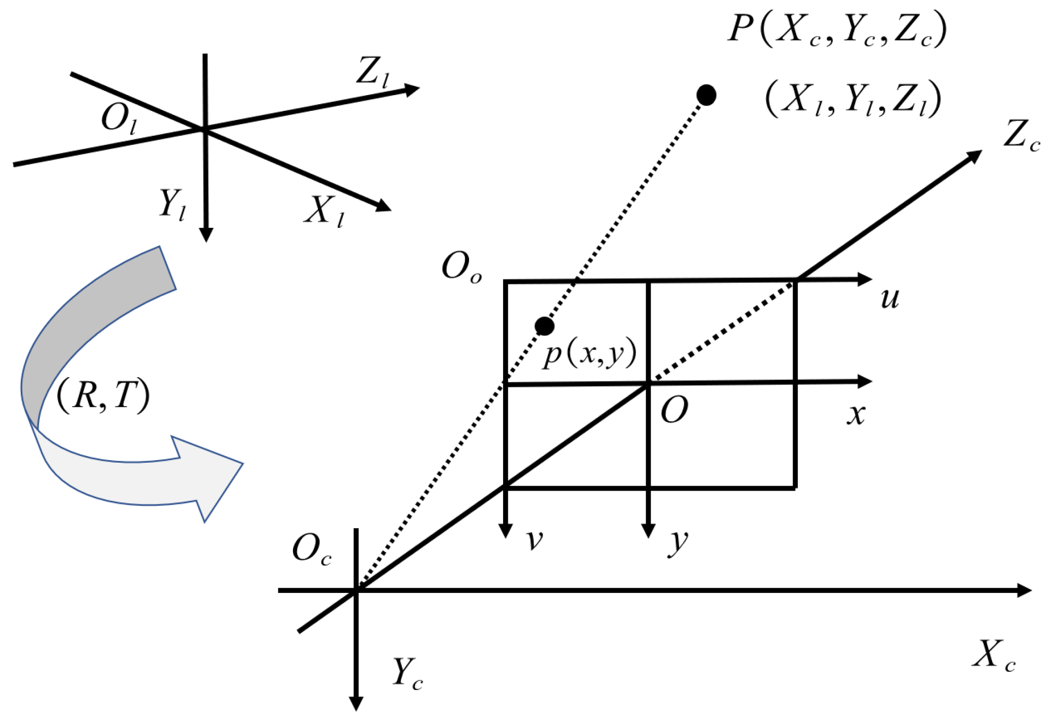
The geometric relationship between the coordinate system of LiDAR point cloud data in three-dimensional space and the pixel coordinate system is described in Figure 1, which includes the coordinate system of LiDAR ($O_l-X_l{Y}_l{Z}_l$), the coordinate system of the camera ($O_c-X_c{Y}_c{Z}_c$), the coordinate system of pixels ($O_o-uv$) and the coordinate system of images ($O-xy$). As shown in the figure, obtaining the rotation parameter R and the translation parameter T is the final task of the whole external parameter calibration process, so that the LiDAR data can be accurately projected to the coordinate system of pixels, thus enabling the data fusion between LIDAR and the camera.

In Figure 1, the point P can be expressed in the camera coordinate system as $P\left(X_c,Y_c,Z_c\right)$, and its coordinates in the pixel system are expressed a $p\left(u,v\right)$. According to the camera imaging principle, the relationship of these three-dimensional coordinates can be expressed as

$$Z_c\left[\begin{array}{c}u\\ v\\ 1\end{array}\right]=\left[\begin{array}{ccc}{f}_x& 0& c_x\\ 0& f_y& c_y\\ 0& 0& 1\end{array}\right]\left[\begin{array}{c}{X}_c\\ Y_c\\ Z_c\end{array}\right]\triangleq K{P}_c$$

(1)

The camera’s internal parameter matrix K can usually be considered as a fixed value. Before starting the experiment, we calibrated the internal parameters of our camera using the conventional method [26]; the obtained K matrix was:

$$K=\left[\begin{array}{ccc}907.09& 0& 648.39\\ 0& 903.97& 331.71\\ 0& 0& 1\end{array}\right]$$

(2)

The point P also can be expressed in the coordinate of LiDAR as $P\left(X_l,Y_l,Z_l\right)$; then:

$$\left[\begin{array}{c}u\\ v\\ 1\end{array}\right]=\frac{1}{Z_c}K\left(R\left[\begin{array}{c}{X}_l\\ Y_l\\ Z_l\end{array}\right]+T\right)$$

(3)

For a calibrated camera, only R and T need to be known to accurately complete the calibration of the two coordinate systems.

3.2. LiDAR–Camera Calibration Method

Considering human eye safety, the interaction with the atmosphere and so on, LiDAR often uses 905 nm and 1550 nm light sources. Because these light sources are not in the visible range band, the camera cannot directly capture the laser spot of LiDAR. Therefore, existing methods based on the calibration of 3D–2D correspondences tend to look for common features (e.g., corner points, circle centers) in LiDAR point cloud data and images. Since this feature extraction method obtains the 3D–2D correspondence between LiDAR and camera at the feature points, there are two main problems. One problem is that there is no simple method to accurately extract features from sparse LiDAR data; the other is that only the 3D–2D correspondence between the LiDAR and the camera at the feature points is obtained.

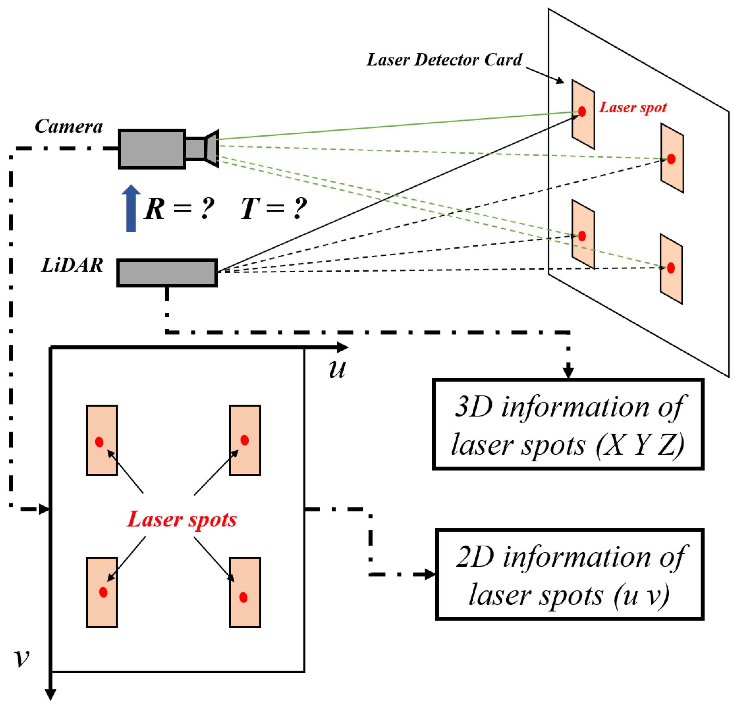
Laser detector cards are made of slowly decaying fluorescent materials that convert invisible light into visible light. Therefore, they make it easy to locate the laser spots formed by the laser beam of the LiDAR on objects and to visualize the spatial pattern graphics. As shown in Figure 2, since the photosensitive area of the laser detector card can clearly observe the laser spots of the LiDAR, these spots can also be captured by the camera, which means that this method can directly obtain the three-dimensional coordinates of each laser spot from the LiDAR and the image coordinates from the camera (i.e., 3D–2D correspondence).

Since the camera can capture the position of the laser spot on the laser detector card, this paper uses the laser detector card as an auxiliary tool to directly obtain the correspondences between laser points and image pixels to complete the calibration of the LiDAR–camera system. As shown in Figure 2, when the laser emitted by LiDAR is pointed at the laser detector card, a laser spot is generated that can be directly observed by the camera. Now, for each laser spot on the laser detector card, the 3D information acquired by LiDAR is $X_l,Y_l,Z_l$ in Equation (3), and the image coordinate information acquired by the camera is $u,v$ in Equation (3).

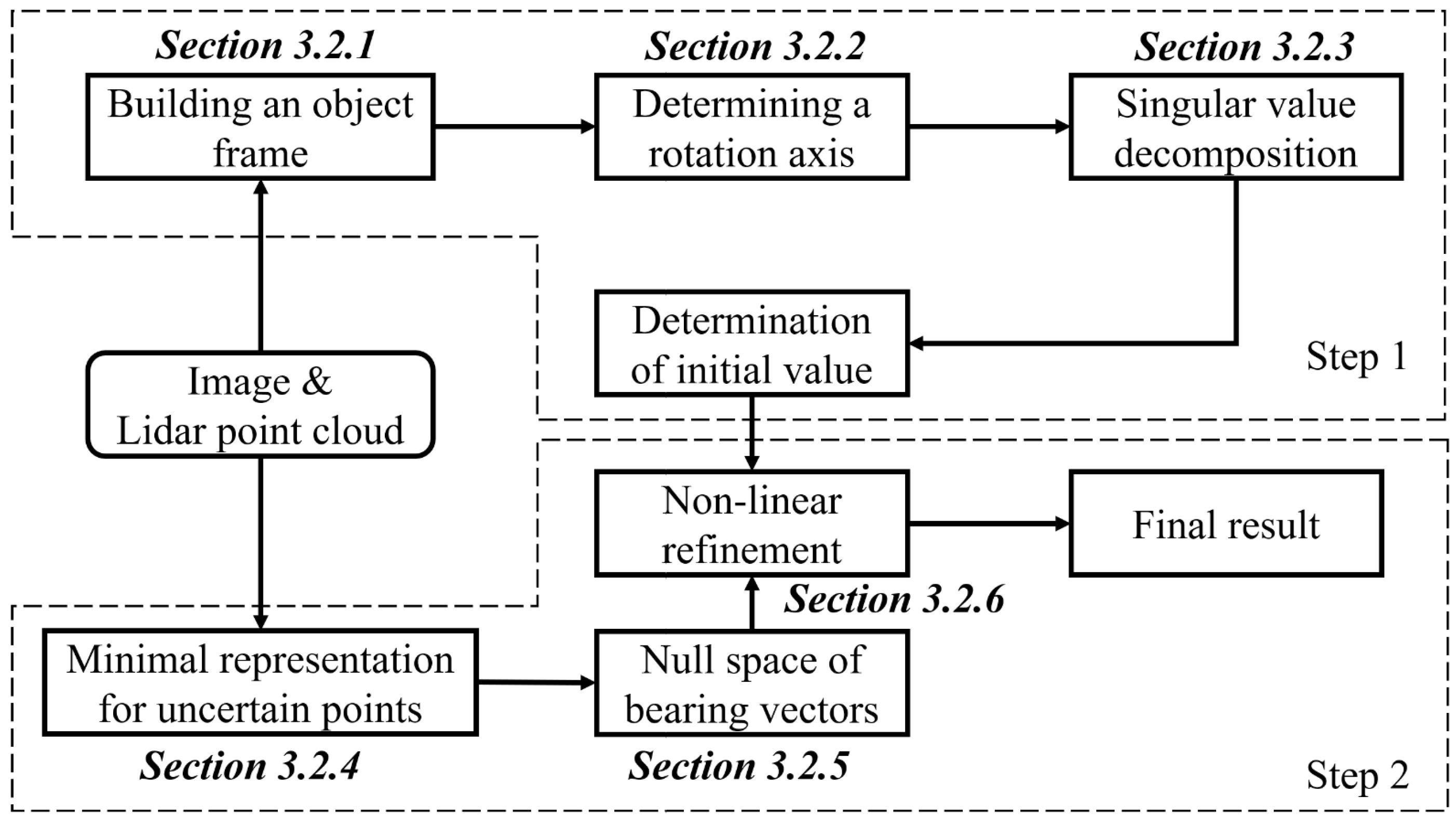
Since 3D coordinates and their image coordinates can be obtained directly, we propose a two-stage framework from coarse to fine (TSPnP) to efficiently utilize these correspondences. After obtaining $X_l,Y_l,Z_l,u,v$, the solution for R and T is analyzed below. Here, we borrow the idea of the PnP algorithm and design a two-stage framework from coarse to fine (called TSPnP), which can complete the accurate external calibration by using only four LiDAR data points and the corresponding pixel information. The main ideas are shown in Figure 3. In the first step, a seventh-order polynomial is constructed by geometric constraints (triangular constraints) to obtain the initial solution quickly. In the second step, the vector tangent space residual equations and the covariance matrix of corresponding observations are constructed by combining the uncertainty of image observations. Finally, the vector tangent space residual is minimized by using the Gauss–Newton iteration method. Since an initial value with higher accuracy is obtained in the first step, the second part requires only one iteration to obtain the high progress result.

3.2.1. Building an Object Frame

As shown in Figure 4, for the calibrated camera, the 3D points $P_i(i=1,\dots ,n)$ acquired by the LiDAR can be converted to the normalized image plane as $p_i(i=1,\dots ,n)$. Among these 3D points, select the two farthest points as the rotation axes ($\overrightarrow{P_i{P}_j}$), and take the midpoint of these two points as the origin of the coordinate system $O_a$; then, the intermediate coordinate system can be established as $\left[O_a-X_a{Y}_a{Z}_a\right]$, where:

$$\overrightarrow{Z_a}=\frac{P_j-O_a}{∥P_j-O_a∥}$$

(4)

If $\left|{\left[0,1,0\right]}^T\overrightarrow{Z_a}\right|⩽\left|{\left[0,0,1\right]}^T\overrightarrow{Z_a}\right|$,

$$\overrightarrow{X_a}=\frac{\overrightarrow{Z_a}\times {\left[0,1,0\right]}^T}{∥\overrightarrow{Z_a}\times {\left[0,1,0\right]}^T∥},\overrightarrow{Y_a}=\frac{\overrightarrow{Z_a}\times \overrightarrow{X_a}}{∥\overrightarrow{Z_a}\times \overrightarrow{X_a}∥}$$

(5)

If $\left|{\left[0,1,0\right]}^T\overrightarrow{Z_a}\right|>\left|{\left[0,0,1\right]}^T\overrightarrow{Z_a}\right|$,

$$\overrightarrow{Y_a}=\frac{{\left[0,0,1\right]}^T\times \overrightarrow{Z_a}}{∥{\left[0,0,1\right]}^T\times \overrightarrow{Z_a}∥},\overrightarrow{X_a}=\frac{\overrightarrow{Y_a}\times \overrightarrow{Z_a}}{∥\overrightarrow{Y_a}\times \overrightarrow{Z_a}∥}$$

(6)

Figure 4. Building an object frame and determining a rotation axis.

Figure 4. Building an object frame and determining a rotation axis.

3.2.2. Determining a Rotation Axis

For n 3D reference points, $P_i$ and $P_j$ can form a three-point set $\left\{P_i,P_j,P_k\left|k\ne i,\right.k\ne j\right\}$ with the remaining (n−2) points. By using the P3P method, each subset can generate a polynomial and the total equation can be expressed as:

$$\left\{\begin{array}{c}{f}_1\left(x\right)=a_1{x}^4+b_1{x}^3+c_1{x}^2+d_{1}x+e_1=0\hfill \\ f_2\left(x\right)=a_2{x}^4+b_2{x}^3+c_2{x}^2+d_{2}x+e_2=0\hfill \\ \dots \hfill \\ f_{n-2}\left(x\right)=a_{n-2}{x}^4+b_{n-2}{x}^3+c_{n-2}{x}^2+d_{n-2}x+e_{n-2}=0\hfill \end{array}\right.$$

(7)

To obtain robust results, the loss function is constructed as $F^{\prime }={\sum }_{i=1}^{n-2}{f}_i\left(x\right)f_i^{{}^{\prime }}\left(x\right)$. The minimum value can be determined by using the singular value decomposition method provided in the literature [27].When the minimum value is obtained, we can calculate the depths of $P_i$ and $P_j$ with the help of the P3P constraint; finally, we can obtain the highly robust rotation axis $Z_a$ [28]: $Z_a=\overrightarrow{P_i{P}_j}/∥P_i{P}_j∥$.

3.2.3. Singular Value Decomposition

After obtaining the $Z_a$ of the $\left[O_a-X_a{Y}_a{Z}_a\right]$, the rotation matrix from $\left[O_a-X_a{Y}_a{Z}_a\right]$ to $\left[O_c-X_c{Y}_c{Z}_c\right]$ is computed as [29]:

$$R_{ac}=R_1{R}_2=\left[\begin{array}{ccc}{r}_1& r_2& r_3\\ r_4& r_5& r_6\\ r_7& r_8& r_9\end{array}\right]\left[\begin{array}{ccc}c& -s& 0\\ s& c& 0\\ 0& 0& 1\end{array}\right]$$

(8)

where $R_1$ is an arbitrary rotation matrix and its ${\left[r_3,r_6,r_9\right]}^T$ is equal to the axis $Z_a$. In addition, $R_1$ is a rotation matrix and, therefore, is an orthogonal matrix. $R_2$ indicates the rotation angle $\alpha$ around the Z-axis, where $c=cos\alpha$, $s=sin\alpha$.

Based on this, the conversion from the 3D point in the intermediate coordinate system to the normalized image plane can be calculated with the following formula:

$${\lambda }_i{f}_i=R_{ac}{P}_i+t_{ac}i=1,2,\dots ,n$$

(9)

where $f_i={\left[u_i{v}_{i}1\right]}^T$, $t_{ac}={\left[t_x{t}_y{t}_z\right]}^T$.

By expanding Equations (8) and (9), we can obtain the following:

$${\lambda }_i\left[\begin{array}{c}{u}_i\\ v_i\\ 1\end{array}\right]=\left[\begin{array}{ccc}{r}_1& r_2& r_3\\ r_4& r_5& r_6\\ r_7& r_8& r_9\end{array}\right]\left[\begin{array}{ccc}c& -s& 0\\ s& c& 0\\ 0& 0& 1\end{array}\right]\left[\begin{array}{c}{X}_i\\ Y_i\\ Z_i\end{array}\right]+\left[\begin{array}{c}{t}_x\\ t_y\\ t_z\end{array}\right]$$

(10)

We arrange all the terms of Equation (10) into a linear system of equations:

$$\left[A_{2n\times 1}{B}_{2n\times 1}{C}_{2n\times 4}\right]{\left[cx{t}_x{t}_y{t}_{z}1\right]}^T=0$$

(11)

where $\left[cs{t}_x{t}_y{t}_{z}1\right]$ are unknown variables, and:

$$A_{2n\times 1}=\left[\begin{array}{c}{u}_1{X}_1{r}_3-Y_1{r}_4-X_1{r}_1+u_1{Y}_1{r}_6\\ v_1{X}_1{r}_3-Y_1{r}_5-X_1{r}_2+v_1{Y}_1{r}_6\\ \dots \\ \dots \\ u_n{X}_n{r}_3-Y_n{r}_4-X_n{r}_1+u_n{Y}_n{r}_6\\ v_n{X}_n{r}_3-Y_n{r}_5-X_n{r}_2+v_n{Y}_n{r}_6\end{array}\right]$$

(12)

$$B_{2n\times 1}=\left[\begin{array}{c}{Y}_1{r}_1+u_1{X}_1{r}_6-u_1{Y}_1{r}_3-X_1{r}_4\\ Y_1{r}_2+u_1{X}_1{r}_6-u_1{Y}_1{r}_3-X_1{r}_5\\ \dots \\ \dots \\ Y_n{r}_1+u_n{X}_n{r}_6-u_n{Y}_n{r}_3-X_n{r}_4\\ Y_n{r}_2+u_n{X}_n{r}_6-u_n{Y}_n{r}_3-X_n{r}_5\end{array}\right]$$

(13)

$$C_{2n\times 4}=\left[\begin{array}{cccc}-1& 0& u_1& u_1{r}_9{Z}_1-r_7{Z}_1\\ 0& -1& v_1& u_1{r}_9{Z}_1-r_8{Z}_1\\ & & \dots & \\ & & \dots & \\ -1& 0& u_n& u_n{r}_9{Z}_n-r_7{Z}_n\\ 0& -1& v_n& u_n{r}_9{Z}_n-r_8{Z}_n\end{array}\right]$$

(14)

For each 3D point, $\left[A_{2n\times 1}{B}_{2n\times 1}{C}_{2n\times 4}\right]$ can be calculated separately. The singular value decomposition (SVD) method is used to solve this linear equation to obtain the value of the unknown variables $\left[cs{t}_x{t}_y{t}_{z}1\right]$. According to Equation (10), the coordinates of point P in the camera coordinate system are recorded as ${\Delta }_i(i=1,\dots ,n)$. We record point P in the LiDAR coordinate system as ${\Lambda }_i(i=1,\dots ,n)$. Therefore, the transformation parameters $R^{*},T^{*}$ between the LiDAR coordinates and the camera coordinates are given by the standard 3D alignment scheme [30]:

$$R^{*},T^{*}=\underset{R,T}{argmin}{e}^2\left(R,T\right)=\underset{R,T}{argmin}\frac{1}{n}{\sum }_{i=1}^n{∥{\Delta }_i-\left(R{\Lambda }_i+T\right)∥}^2$$

(15)

Above, we obtained the initial value of the LiDAR and camera system external parameters, which is $R^{*},T^{*}$.

3.2.4. Minimal Representation for Uncertain Points

If a laser spot occupies only one pixel (as shown in Figure 5a), then the pixel information at this point is determined. However, in the actual system, due to the interference of astigmatism and stray light, the light spot may occupy several pixels (as shown in Figure 5b,c).At this time, there is an error between the pixel information of the laser spot extracted by the classical centroid extraction method (equation) and the actual pixel information of the laser spot. Because it is difficult to determine the true error, we compare the calculated gray value of the laser spot with the gray value of its neighborhood to determine the uncertain area of the laser spot, and finally obtain the uncertain representation of the pixel information of the laser spot:

$$\left\{\begin{array}{c}{\sigma }_{u^{\prime }}=argmax\sqrt{{\left(u-u^{\prime }\right)}^2}\hfill \\ {\sigma }_{v^{\prime }}=argmax\sqrt{{\left(v-v^{\prime }\right)}^2}\hfill \\ s.t.\left|I\left(u,v\right)-I\left(u^{\prime },v^{\prime }\right)\right|<{\epsilon }_I\hfill \end{array}\right.$$

(16)

where

$$u^{\prime }=\frac{{\sum }_{\left(u_i,v_j\right)\in area}{u}_i·I\left(u_i,v_j\right)}{{\sum }_{\left(u_i,v_j\right)\in area}I\left(u_i,v_j\right)},v^{\prime }=\frac{{\sum }_{\left(u_i,v_j\right)\in area}{v}_i·I\left(u_i,v_j\right)}{{\sum }_{\left(u_i,v_j\right)\in area}I\left(u_i,v_j\right)}$$

(17)

The idea of refinement is shown in Figure 6. Ideally, the space point $P_i$ is projected to the point $p_i$ on the image plane of the camera. However, due to the uncertainty of image observation (such as errors in feature point extraction, etc.), the final calculation result is obtained as point ${\widehat{p}}_i$ and the calculated $\overrightarrow{O_c{\widehat{p}}_i}$ has a residual in the tangent space of $P_i$ (the tangent space is composed of $m_i$ and $n_i$ ). Based on this, we discuss how to minimize this residual.

We propagate the uncertainty of the two-dimensional images to direction vectors (normalized coordinates) and obtain linear solutions with non-singular covariance matrices by reducing the observation space provided by Ref. [30]. As shown in Figure 6, the 3D point $P_i$ measured by the LiDAR is observed through the calibrated camera, and the uncertainty of the observed points can be expressed by a two-dimensional covariance matrix, which yields:

$$X^{\prime }=\left[\begin{array}{c}{u}^{\prime }\\ v^{\prime }\end{array}\right],{\sum }_{X^{\prime }{X}^{\prime }}=\left[\begin{array}{cc}{\sigma }_{u^{\prime }}^2& 0\\ 0& {\sigma }_{v^{\prime }}^2\end{array}\right]$$

(18)

where ${\left[\begin{array}{cc}{u}^{\prime }& v^{\prime }\end{array}\right]}^T$ is the coordinates of point ${\widehat{p}}_i$ and ${\sum }_{X^{\prime }{X}^{\prime }}$ is the uncertainty of the coordinate.

Next, we generalize the uncertainty of the points in the image to the uncertainty of the points in space. Using the forward projection function, the image point $X^{\prime }$ can be projected to the corresponding 3D vector in camera coordinates and $J_{\pi }$ is the Jacobi matrix of the positive projection. Therefore, the uncertainty of the 3D vector obtained after performing the projection transformation is:

$$X=K^{-1}{X}^{\prime },J_{\pi }=\left[\begin{array}{cc}\frac{\partial {\pi }_{u^{\prime }}}{\partial u^{\prime }}& \frac{\partial {\pi }_{u^{\prime }}}{\partial v^{\prime }}\\ \frac{\partial {\pi }_{y^{\prime }}}{\partial v^{\prime }}& \frac{\partial {\pi }_{v^{\prime }}}{\partial v^{\prime }}\\ 0& 0\end{array}\right]$$

(19)

Since the depth information of point x is missing, we need to normalize the points obtained by projection, that is, normalization of Equation (19). Therefore, the final observations are obtained by normalizing Equation (19) and noting the orientation vectors [31]:

$$\mathbf{V}=\left[\begin{array}{c}{v}_x\\ v_y\\ v_z\end{array}\right]=\frac{X}{∥X∥},{\mathbf{\sum }}_{\mathbf{vv}}=\mathrm{J}{\sum }_{\mathbf{xx}}{\mathrm{J}}^{\mathrm{T}},\mathrm{J}=\frac{1}{∥X∥}\left({\mathrm{I}}_3-{\mathrm{vv}}^{\mathrm{T}}\right)$$

(20)

where V is the unit vector of $\overrightarrow{O_c{\widehat{p}}_i}$ and ${\mathbf{\sum }}_{\mathbf{VV}}$ is the three-dimensional uncertainty of vector V (called residual in the tangent space ).

3.2.5. Null Space of Bearing Vectors

As shown in Figure 6, the null space is composed of two vertical vectors, m and n. The null space is perpendicular to $\overrightarrow{O_c{\widehat{p}}_i}$, that is, the null space in the tangent space of $\overrightarrow{O_c{\widehat{p}}_i}$:

$$J_{V_r}=null\left(v^T\right)=\left[\begin{array}{cc}m& n\end{array}\right]=\left[\begin{array}{cc}\begin{array}{c}{m}_1\\ m_2\end{array}& \begin{array}{c}{n}_1\\ n_2\end{array}\\ m_3& n_3\end{array}\right]$$

(21)

In its tangent space, we can obtain tangent space representation and residuals in tangent space [31]:

$$V_r=\left[\begin{array}{c}dm\\ dn\end{array}\right]=J_{v_r}^T\left(v\right)V=\left[\begin{array}{c}0\\ 0\end{array}\right]$$

(22)

$${\sum }_{v_r{v}_r}=J_{v_r}^T\left(v\right){\sum }_{\mathit{vv}}{J}_{v_r}^{}\left(v\right)=\left[\begin{array}{cc}{\sigma }_{v_{r_x}}^2& {\sigma }_{v_{r_{xy}}}^2\\ {\sigma }_{v_{r_{yx}}}^2& {\sigma }_{v_{r_y}}^2\end{array}\right]$$

(23)

3.2.6. Non-Linear Refinement

Combining Equation (22) and the camera projection model, we can obtain the projection model in tangent space:

$$\left[\begin{array}{c}{d}_m\\ d_n\end{array}\right]=\left[\begin{array}{c}{m}^T\\ n^T\end{array}\right]{\lambda }_i^{-1}\left({RP}_i+T\right)=0$$

(24)

Equation (24) is satisfied for every point in the space; hence:

$$\begin{array}{cc}\hfill 0& =m_1({\widehat{r}}_{11}{P}_x+{\widehat{r}}_{12}{P}_y+{\widehat{r}}_{13}{P}_z+{\widehat{t}}_1)\hfill \\ & + m_2({\widehat{r}}_{21}{P}_x+{\widehat{r}}_{22}{P}_y+{\widehat{r}}_{23}{P}_z+{\widehat{t}}_2)\hfill \\ & + m_3({\widehat{r}}_{31}{P}_x+{\widehat{r}}_{32}{P}_y+{\widehat{r}}_{33}{P}_z+{\widehat{t}}_3)\hfill \\ \hfill 0& =n_1({\widehat{r}}_{11}{P}_x+{\widehat{r}}_{12}{P}_y+{\widehat{r}}_{13}{P}_z+{\widehat{t}}_1)\hfill \\ & + n_2({\widehat{r}}_{21}{P}_x+{\widehat{r}}_{22}{P}_y+{\widehat{r}}_{23}{P}_z+{\widehat{t}}_2)\hfill \\ & + n_3({\widehat{r}}_{31}{P}_x+{\widehat{r}}_{32}{P}_y+{\widehat{r}}_{33}{P}_z+{\widehat{t}}_3)\hfill \end{array}$$

(25)

Since Equation (25) is a linear system of equations, we can recombine them to obtain homogeneous linear equations:

$$Du=0,E=\left[\begin{array}{ccc}{\sum }_{v_r^1{v}_r^1}^{-1}& \cdots & 0\\ ⋮& \ddots & ⋮\\ 0& \cdots & {\sum }_{v_r^i{v}_r^i}^{-1}\end{array}\right]$$

(26)

where $u={[{\widehat{r}}_{11},{\widehat{r}}_{12},{\widehat{r}}_{13},{\widehat{r}}_{21},{\widehat{r}}_{22},{\widehat{r}}_{23},{\widehat{r}}_{31},{\widehat{r}}_{32},{\widehat{r}}_{33},{\widehat{t}}_1,{\widehat{t}}_2,{\widehat{t}}_3]}^T$. The matrix D can be calculated separately. The matrix E is the overall covariance matrix consisting of the covariance of V corresponding to each point, such that our model incorporates the observed uncertainty. To minimize the tangent space residuals in Equation (24), we arrive at the following least-squares problem:

$$u=\underset{u}{argmin}\widehat{\epsilon }=\underset{u}{argmin}DuEDu$$

(27)

We use the values of $R^{*}$, $T^{*}$ obtained in Section 3.2.3 as the initial values of u. Furthermore, $R^{*}$ is expressed as the Cayley parameter to obtain a minimal representation of the rotation matrix in this paper. Next, the Gauss–Newton method is used to solve the above problem, using only one iteration, since the initial value $R^{*}$, $T^{*}$ is sufficiently accurate.

4. Results

4.1. Simulations Results

In this section, the performance of the proposed method (called TSPnP) is analyzed using synthetic data and its accuracy is compared with existing methods:

LHM: the computational results usually converge; one of the most classical iterative methods [32];

EPnP: an efficient non-iterative method when n > 6 [33];

RPnP: a fast and robust method for solving PnP [34];

DLS: a unique nonlinear least squares cost function; its performance is close to that of the maximum likelihood (MLE) method [35];

OPnP: the calculation result is globally optimal [36];

MLPnP: a maximum likelihood solution method for the PnP problem when n > 6 [37];

SRPnP: low-cost computing methods [29].

4.1.1. Synthetic Data

A virtual perspective camera was created; the image size of the camera was 640 × 480 pixels, the focal length of the camera was 800 pixels, and main point was located at the center of the image. Next, we generated n 3D reference points in the camera frame and used the true values of rotation and translation to convert these 3D points into world frames. Finally, we used the calibrated virtual camera to project these 3D points onto the 2D image plane. According to previous studies, two types of Gaussian white noise were added to the 2D image plane, one for all pixels on the image obeying a Gaussian white noise with mean 0 and variance $\sigma$ (Noise Level 1), and the other for the pixel points on the image obeying a Gaussian white noise with mean 0 and variance between 0 and $\sigma$ (Noise Level 2) [38].

The accuracy of the solution result of the PnP problem is strongly related to the distribution of the 3D reference points; thus, we need to distribute different locations to test the proposed method. We used matrix $M={\left[W_1,W_2,\dots ,W_n\right]}^T$ to express the generated point coordinates, where $W_i$ is the 3D coordinates and n is the number of points.

Let the matrix $M={\left[W_1,W_2,\dots ,W_n\right]}^T$, where $W_i$ is the 3D coordinates of the reference points and n is the size of the point set. According to the rank and eigenvalues of the 3 × 3 matrix $M^{T}M$, the distribution of points can be divided into three groups:

(1) Ordinary case: $rank\left(M^{T}M\right)=3$ and all eigenvalues of $M^{T}M$ are not close to zero. Eventually, these points are scattered in the region of [−2, 2] × [−2, 2] × [4, 8];

(2) Planar case: $rank\left(M^{T}M\right)=2$. In this situation, these points are in a plane, and we may scatter these points in the region of [−2, 2] × [−2, 2] × [0, 0];

(3) Quasi-singular case: $rank\left(M^{T}M\right)=3$ and the minimum eigenvalue is much smaller than the maximum eigenvalue. Its ratio is less than 0.05. Eventually, these points are scattered in the region of [1, 2] × [1, 2] × [4, 8].

The error of the calculated rotation parameter R and translation parameter T is calculated as follows:

$$e_{rot}\left(degrees\right)=\underset{k\in \left\{1,2,3\right\}}{max}{cos}^{-1}\left(r_{k,true}^T{r}_k\right)\times \frac{180}{\pi }$$

(28)

$$e_{trans}\left(\%\right)=\frac{∥t_{true}-t∥}{∥t∥}\times 100$$

(29)

where $r_{k,true}^{}$ is the kth columns of $R_{true}$ and $r_k^{}$ is the kth columns of R.

4.1.2. Performance under Different Number of Points

We first design simulation experiments to evaluate the performance of all methods with different number of points. The number of points is gradually increased from 6 to 20 and zero-mean Gaussian noise with a fixed deviation $\delta$ = 2 pixels is added to the image. From the results in Figure 7, it can be seen that EPnP (and, in general, EPnP+GN) is not accurate enough due to its potential linearization scheme, especially when n is very small. RPnP performs poorly in many cases because it is not an optimal calculation method. In the quasi-singular and planar cases, the accuracy of the LHM is much lower. In addition, when the number of points is relatively small, the results of LHM may be wrong because there may be a local optimum. Due to the singularity of the Cayley parameters, the DLS method is unstable for the proposed singular and planar cases. MLPnP is equally unstable for the proposed singular and planar cases. Compared to the most advanced and available methods, the accuracy of TSPnP, OPnP and SRPnP are comparable; in the quasi-singular case, the rotation matrix of TSPnP is slightly better than that of the OPnP and SRPnP methods.

4.1.3. Performance under Different Noise

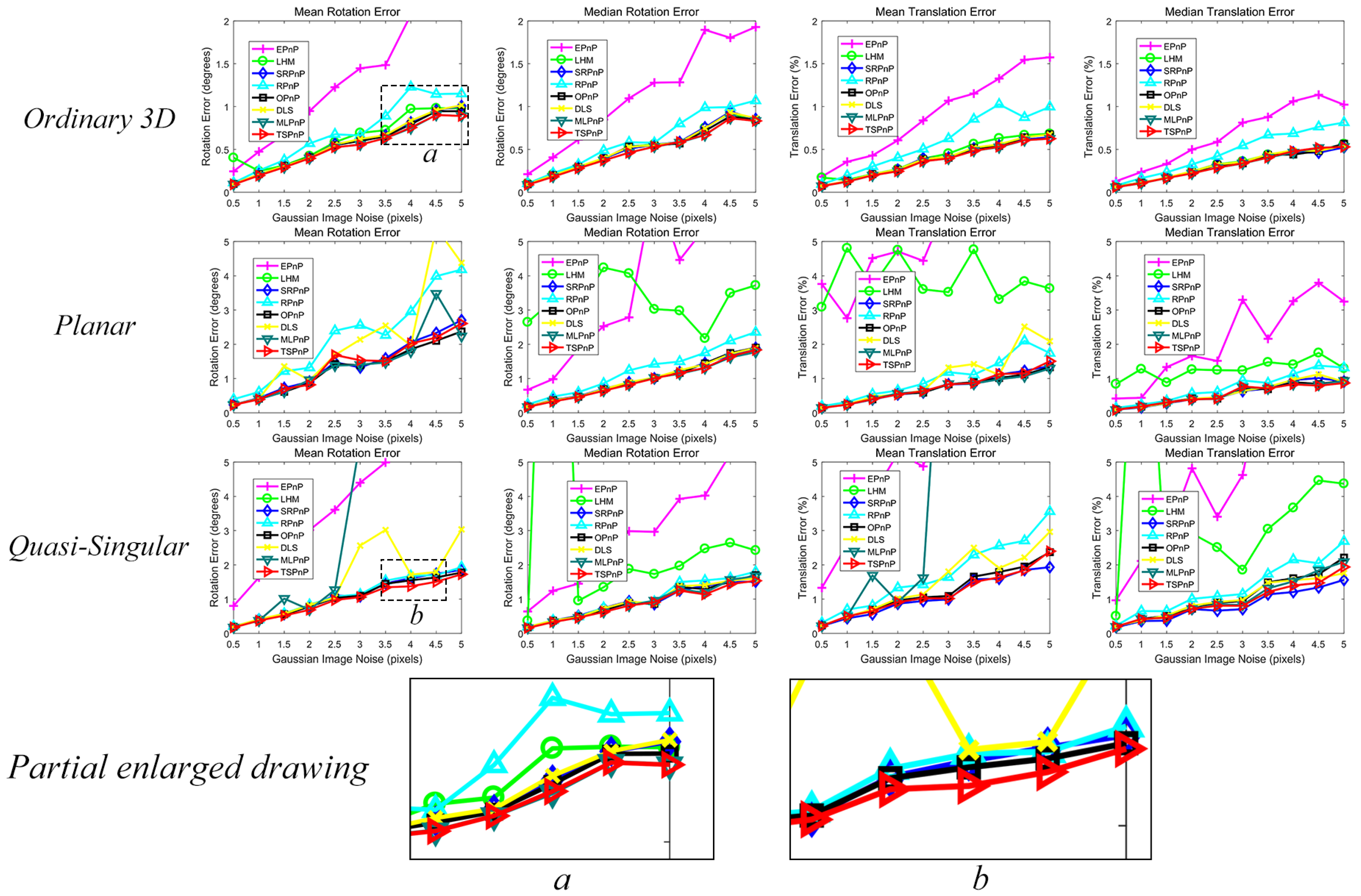
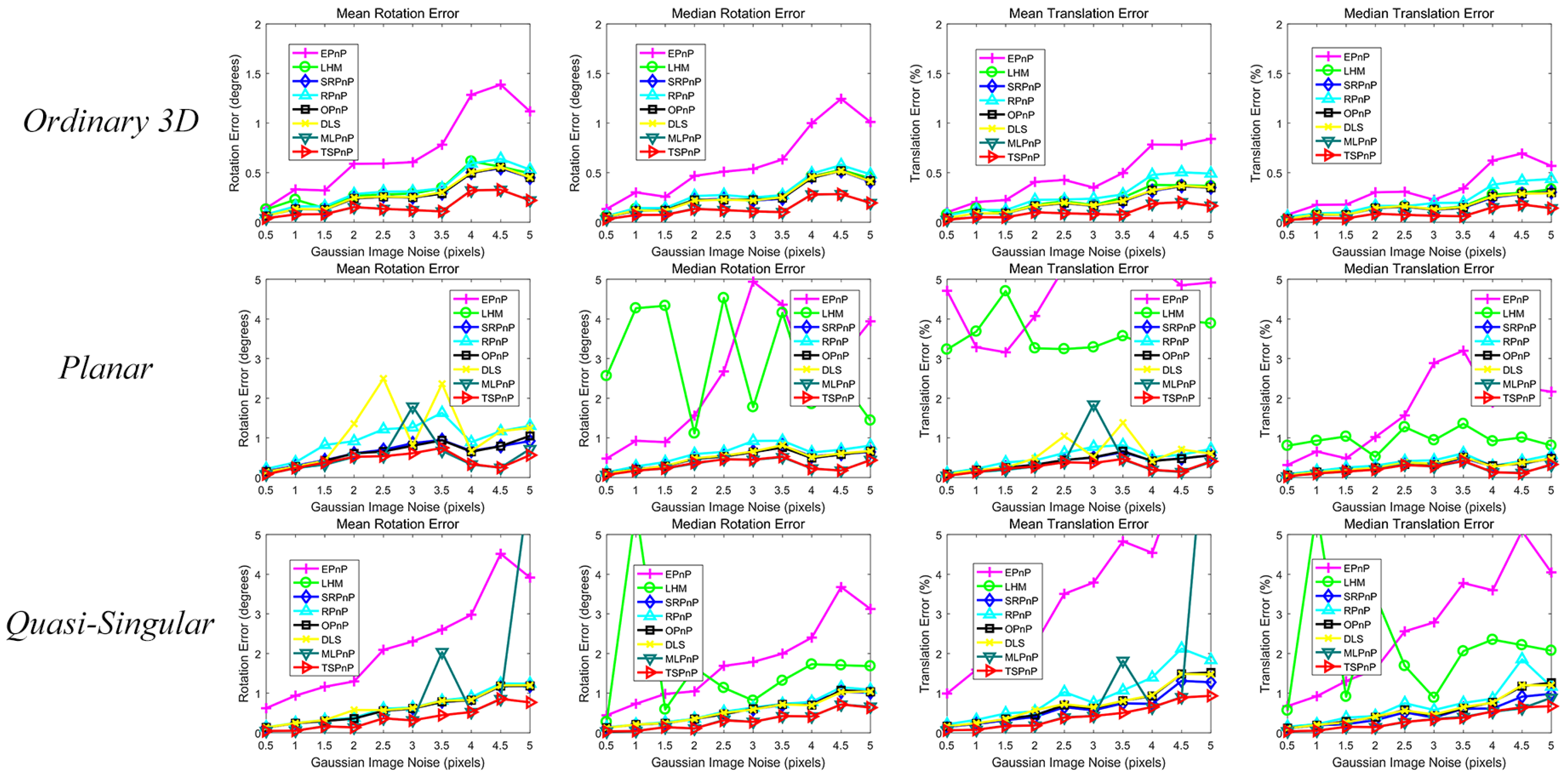
This simulation experiment was designed to test the effect of noise on the accuracy of all methods. Therefore, number of points was fixed (n = 10) and the noise deviation level $\delta$ was gradually increased from 0.5 pixels to 5 pixels. This can be seen from the results in Figure 8. The results also show that TSPnP, OPnP and SRPnP are excellent in all situations and still far superior to other methods in terms of accuracy. In addition, TSPnP has a slightly better rotation matrix than the OPnP and SRPnP methods in the mean rotation error of the ordinary case and a better rotation matrix than the OPnP and SRPnP methods in the mean rotation error of the quasi-singular case.

The third simulation experiment similarly tested the effect of noise on the accuracy of all methods, keeping the number of points constant (n = 10) and increasing the noise bias level $\delta$ from 0.5 pixels to 5 pixels. However, for the noise deviation level $\delta$, a number from 0 to $\delta$ was chosen randomly for each point as the Gaussian distribution variance. That is, the Gaussian distribution variance of all pixel points was not the same, but the variance of the Gaussian distribution of each pixel point was distributed uniformly from 0 to $\delta$. This can be seen from the results in Figure 9, TSPnP and MLPnP were exceptional in these cases, and in terms of accuracy, TSPnP and MLPnP were still far better than other methods. In addition, TSPnP was more stable than MLPnP in the planar case and quasi-singular case.

4.1.4. Computational Efficiency

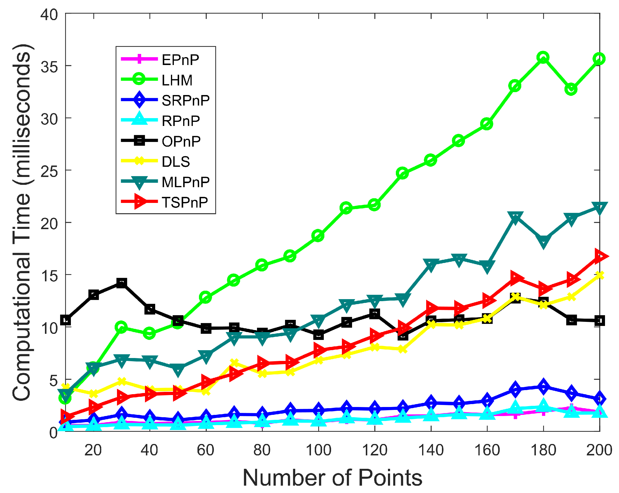
The proposed TSPnP method only needs one iteration; therefore, it has an advantage over the iterative algorithm in terms of computational efficiency. For this reason, this paper conducted experiments to compare the calculation times of the algorithms, as shown in Figure 10. The reference number of points n was varied from 10 to 1000, again adding Gaussian noise with zero mean and standard deviation of d = 2 pixels, and the experiment was repeated 500 times independently. Figure 10 represents the average computation time for these 500 experiments. It can be seen from Figure 10 that although the efficiency of our proposed algorithm execution decreases as the number of estimation points increases, the estimation accuracy becomes higher. Compared with other methods, our algorithm executes more efficiently than the iterative algorithms LHM and MLPnP and the non-iterative algorithm OPnP when the number of points is below 130. While the execution efficiency is lower than EPnP, RPnP, SRPnP and OPnP when the number of points exceeds 130, our algorithm is more robust and can consistently obtain high accuracy results with various noises. Moreover, since the method proposed in this paper uses only four reference points and almost reaches the fastest speed of existing algorithms when the number of points is small, the proposed method is efficient.

4.2. Real Data Results

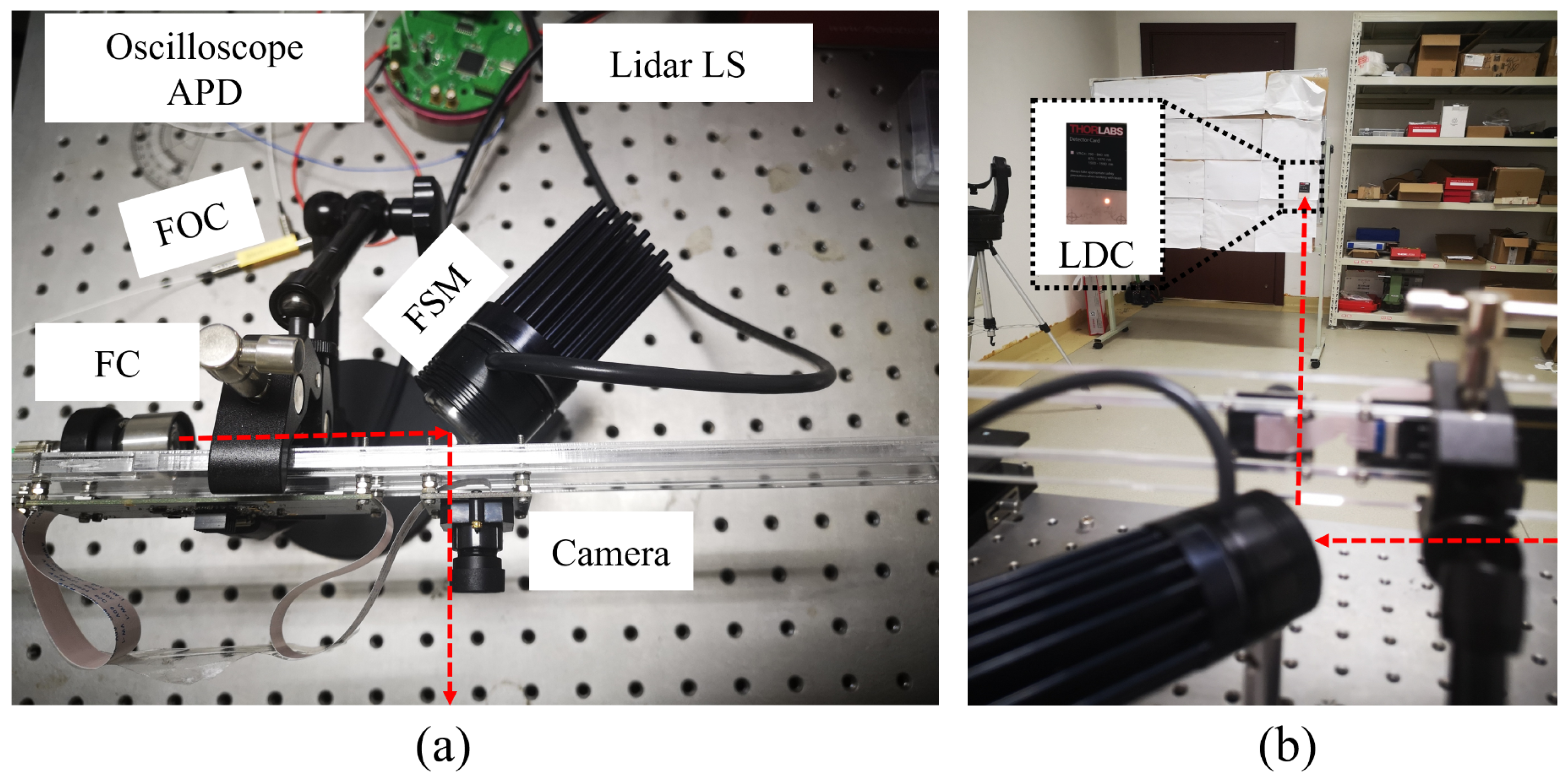
In the experiment, we used a 1550 nm LiDAR based on fast mirror scanning and a common visible light camera with a resolution of 1280 × 720. Specifically, a real LiDAR camera system (as shown in Figure 11a) was built to evaluate the practical application of our proposed method. The LiDAR light source (LiDAR LS) enters from Port 1 of the fiber optic circulator (FOC), exits from Port 2 of FOC, and finally is emitted into free space through the fiber-collimator (FC). When the laser is emitted from the fiber collimator into free space, a reflection occurs, at which time the reflected light enters through the fiber from FOC Port 2, and the laser that enters from FOC Port 2 is output from FOC Port 3. The light output from FOC Port 3 is connected to the APD detector to generate an electrical signal, at which point the electrical signal is collected with an oscilloscope and the emission time $T_1$ of the laser is recorded. The laser in free space is deflected by the fast-steering mirror (FSM); when the deflected laser light hits the surface of the object, part of the laser will re-enter the FC after reflection, and the laser that re-enters the collimator will likewise enter the APD detector through the FOC, at which point the time $T_2$ is recorded by the oscilloscope. The three-dimensional information of the laser point irradiated on the object can be obtained from the time $T_1$, $T_2$ and the angular information of the FSM.

The calibration experiment is shown in Figure 11b. When the laser emitted from the LiDAR is pointed at the laser detector card (LDC), it generates a laser spot that can be directly observed by the camera; at this time, the 3D–2D correspondences between the LIDAR and the camera can be directly obtained. In the next experiment, we randomly placed the laser detector card at four locations in space and recorded the three-dimensional coordinates of the laser point when it was on the laser detector card while the camera captured the pixel information of the laser point at this time, finally obtaining the data shown in

Table 2. Four LiDAR data points and the corresponding pixel information.

Point Index	u	v	X(m)	Y(m)	Z(m)
$P_0$	705	415	−0.184	0	2.105
$P_1$	620	323	0	0.312	3.571
$P_2$	456	401	0.628	0	3.560
$P_3$	701	409	−0.313	0	3.582

.

To evaluate the accuracy of our method, we compared the methods in Section 4.1 that can solve the PnP problem with only four LiDAR points with our method. In addition, data from 10 additional LiDAR points were introduced as evaluation references, and the reprojection errors of these 14 points were used to quantitatively assess the accuracy of our proposed calibration method. The reprojection errors are shown in

Table 3. Reprojection error compared to other calibration methods.

Method	Mean $\left|\mathit{u}\right|$ (Pixel)	Mean $\left|\mathit{v}\right|$ (Pixel)	Mean $\sqrt{{\mathit{u}}^2+{\mathit{v}}^2}$ (Pixel)
TSPnP	1.35	1.21	1.92
OPnP	1.11	1.63	2.07
SRPnP	1.68	1.70	2.51
RPnP	1.11	1.64	2.08

. Although OPnP and RPnP had the best performance on u, they were lower than TSPnP in the v direction and in $\sqrt{u^2+v^2}$. Overall, TSPnP was better than the other methods.

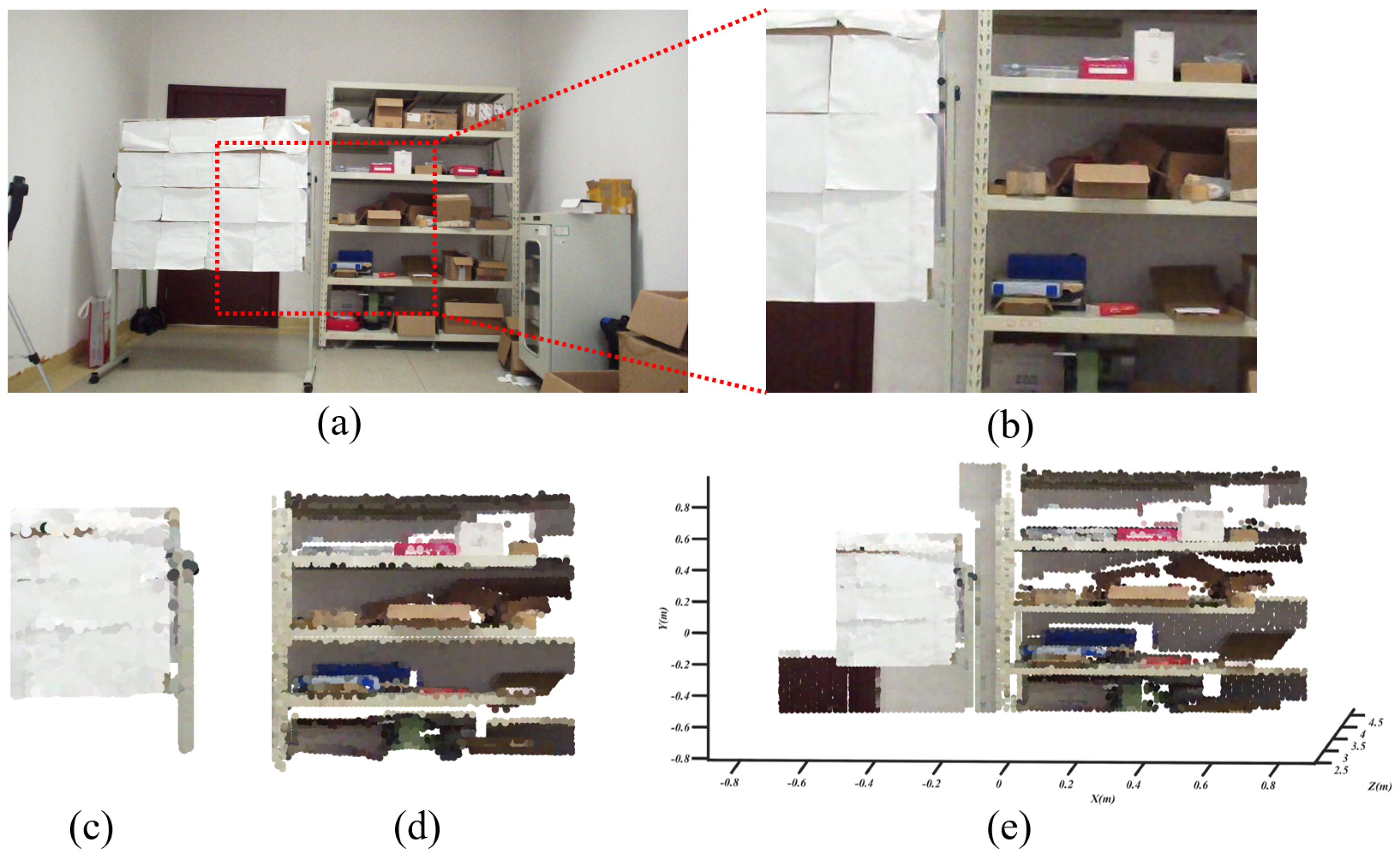
Finally, according to the results obtained by the calibration method in this paper, the RGB colors of the images were mapped to the LiDAR point cloud for data fusion; the results obtained are shown in Figure 12 and Figure 13. From the point cloud data in the Figure 12, the color information of the target can be seen, such as whiteboard, red boxes, etc. From the point cloud data in the Figure 13, the 3D information and color information of the doll are well displayed. This further proves that the color information of the real scene is well mapped to the LiDAR point cloud data. Thus, the proposed method of geometric calibration for the LiDAR–camera system using direct 3D–2D correspondences can efficiently obtain accurate calibration results with only four LiDAR data points and the corresponding pixel information.

4.3. Comparison with Other Calibration Methods

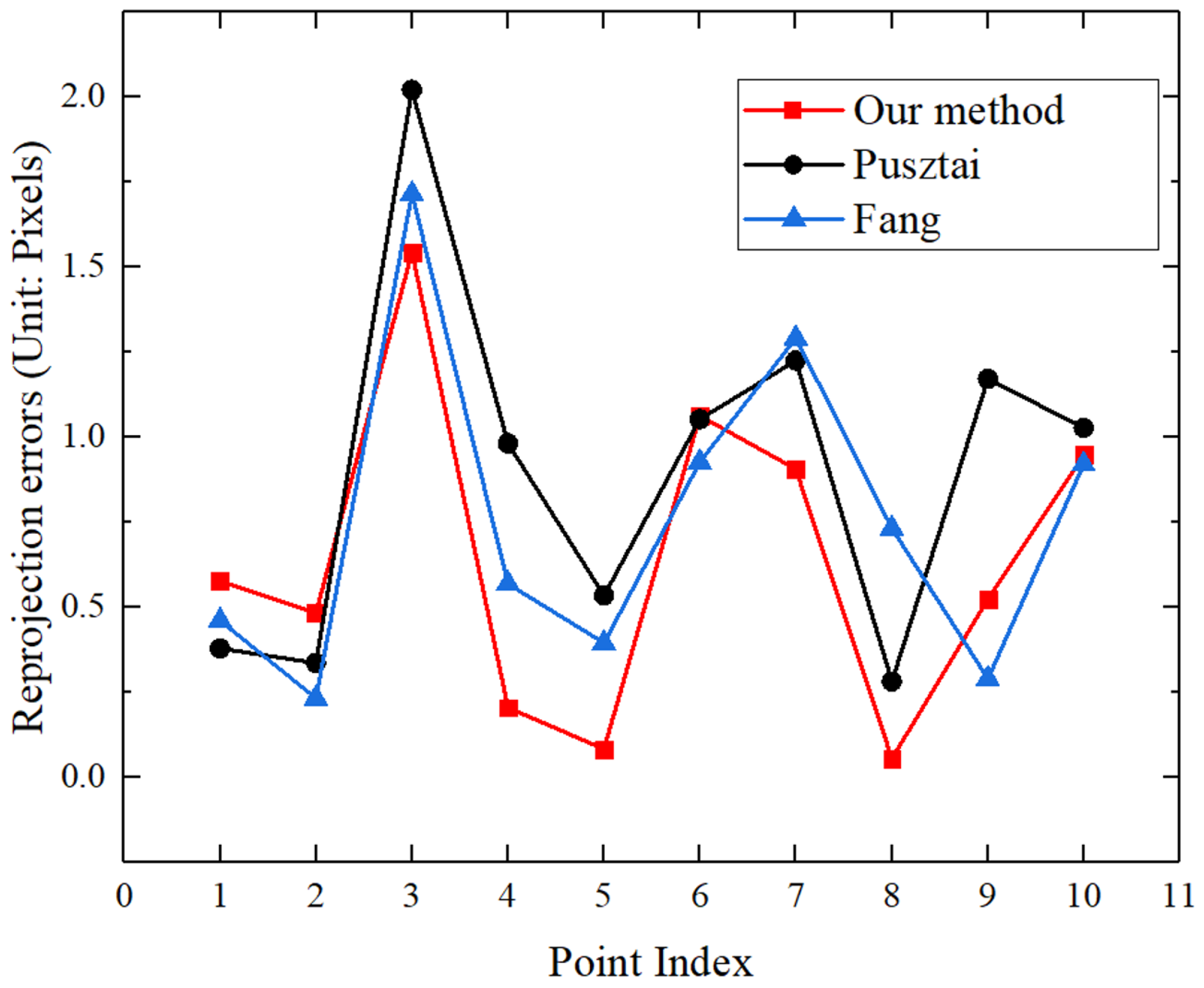
The performance of different calibration methods for LiDAR–camera systems was studied in this experiment. We compared our method with that of Pusztai et al. [39] and Fang et al. [40]. Pusztai used a simple cardboard box with a known size as an auxiliary calibration object, and then extracted corner features to obtain 3D–2D point correspondence, thereby obtaining the external parameters of the LiDAR–camera system. Fang used panoramic infrastructure and a circular mark rather than the apriltag mark as the calibration object, and obtained the 3D–2D point correspondence by extracting the center of the circle and the environmental structural features, thereby obtaining the external parameters of multiple cameras and LiDAR. Our method used the laser detector card as the auxiliary object. With the 3D information of the laser spots obtained by LiDAR, the camera can directly capture the laser spots in the laser sensitive area to obtain the corresponding 2D information, thereby obtaining the external parameters of the LiDAR–camera system. The re-projection error of these methods is shown in Figure 14. It was found that the re-projection error of our method is smaller than that of the other two methods; this is because the other methods all need to extract features from the data to indirectly complete the calibration, and Pusztai’s method requires additional internal parameters known in advance. The average re-projection errors of our method and the other two methods were 0.64 pixels, 0.90 pixels and 0.75 pixels, respectively, Therefore, our method using direct 3D–2D correspondences can achieve more accurate calibration results.

5. Discussion

LiDAR–camera calibration is used to find the spatial conversion relationship between LiDAR and a camera, that is, the rotation matrix R and the translation matrix T required for conversion between different coordinate systems, to prepare for the fusion of LiDAR and camera data. Currently available high-precision calibration methods rely on finding common features in point cloud data and image data; however, most LiDAR point cloud data is not dense enough to easily find key features.

Based on this, the advantages of the method proposed in this paper are:

1.

No need to process sparse LiDAR data (e.g., feature extraction of targets). This paper proposes the use of a laser detector card as an auxiliary tool. Since the laser detector card can convert an invisible laser into a visible laser, for each laser spot, the 3D–2D correspondence can be obtained directly (that is, the 3D information of the laser spot and the pixel information of the laser spot can be obtained at the same time);

2.

Since the proposed method does not need to extract key features of the target from sparse point cloud data, this method can be adapted to more types of LiDAR;

3.

The observation error of the image is taken into account when establishing the calibration model. A two-stage framework from coarse to fine (TSPnP) is proposed to solve the PnP problem with observation errors. Since image observation errors are widely present in practical applications, solving the PnP problem with observation errors will improve the calibration results in practical real-world application scenarios.

In simulation experiments, by varying the pixel error size and the number of 3D–2D point pairs, we compared the proposed TSPnP with the current state-of-the-art PnP methods. The results show that, thanks to the fact that TSPnP takes the image observation error into account, the method outperforms other methods in most cases. In addition, real calibration experiments demonstrated that the proposed TSPnP method is effective and the reprojection errors obtained are smaller than those of other methods. Finally, by comparing the proposed calibration method with other currently available calibration methods in real experiments, it was found that our proposed method outperforms other calibration methods because our method can directly obtain the 3D–2D correspondence, avoiding the secondary errors arising from the process of finding the key features of the target from sparse LiDAR data in other methods.

Despite the unique advantages of our proposed method, it also has some shortcomings:

1.

The calibration method studied in this paper is based on the application scenario of offline calibration; extending this method to application scenarios that require online calibration such as smart driving is something we will try to undertake in the future;

2.

The measurement error of LiDAR is not considered, which also affects the actual calibration results; in the future, we will try to add this error to the calibration model;

3.

We only use the direct 3D–2D correspondence for calibration; in the future, we plan to fuse the direct 3D–2D correspondence and the indirect 3D–2D correspondence to improve robustness and accuracy.

6. Conclusions

In this paper, we proposed a method to directly obtain 3D–2D correspondences between LiDAR and a camera to complete the calibration. We use a laser detector card as an auxiliary tool to directly obtain the laser point–image pixel correspondence, thus solving the problem of difficulty in extracting features from sparse LiDAR data. In addition, we designed a two-stage framework from coarse to fine, which not only can solve the perspective-n-point problem with observation errors, but also requires only four LiDAR data points and the corresponding pixel information for accurate external calibration. Extensive simulations and experiments demonstrated that the effectiveness and accuracy of the proposed method are better than those of existing methods, and the proposed method is accurate enough to adapt to the calibration of most LiDAR and camera systems. In addition, we used the calibration results obtained by our method to map the RGB colors of the image to the LiDAR point cloud for data fusion; the results show that the performance of our method on LiDAR–camera systems is suitable for 3D reconstruction of scenes.

References

- Lin, S.; Garratt, M.A.; Lambert, A.J. Monocular vision-based real-time target recognition and tracking for autonomously landing an UAV in a cluttered shipboard environment. Auton. Robot. 2017, 41, 881–901. [Google Scholar] [CrossRef]
- Li, Y.J.; Zhang, Z.; Luo, D.; Meng, G. Multi-sensor environmental perception and information fusion for vehicle safety. In Proceedings of the 2015 IEEE International Conference on Information and Automation, Lijiang, China, 8–10 August 2015; IEEE: Piscataway, NJ, USA, 2015; pp. 2838–2841. [Google Scholar]
- Gao, H.; Cheng, B.; Wang, J.; Li, K.; Zhao, J.; Li, D. Object classification using CNN-based fusion of vision and LIDAR in autonomous vehicle environment. IEEE Trans. Ind. Inform. 2018, 14, 4224–4231. [Google Scholar] [CrossRef]
- Geng, K.; Dong, G.; Yin, G.; Hu, J. Deep dual-modal traffic objects instance segmentation method using camera and lidar data for autonomous driving. Remote Sens. 2020, 12, 3274. [Google Scholar] [CrossRef]
- An, P.; Ma, T.; Yu, K.; Fang, B.; Zhang, J.; Fu, W.; Ma, J. Geometric calibration for LiDAR-camera system fusing 3D-2D and 3D-3D point correspondences. Opt. Express 2020, 28, 2122–2141. [Google Scholar] [CrossRef] [PubMed]
- Gong, X.; Lin, Y.; Liu, J. Extrinsic calibration of a 3D LIDAR and a camera using a trihedron. Opt. Lasers Eng. 2013, 51, 394–401. [Google Scholar] [CrossRef]
- Liu, H.; Qu, D.; Xu, F.; Zou, F.; Song, J.; Jia, K. Approach for accurate calibration of RGB-D cameras using spheres. Opt. Express 2020, 28, 19058–19073. [Google Scholar] [CrossRef] [PubMed]
- Nguyen, A.D.; Nguyen, T.M.; Yoo, M. Improvement to LiDAR-camera extrinsic calibration by using 3D–3D correspondences. Optik 2022, 259, 168917. [Google Scholar] [CrossRef]
- Lai, Z.; Wang, Y.; Guo, S.; Meng, X.; Li, J.; Li, W.; Han, S. Laser reflectance feature assisted accurate extrinsic calibration for non-repetitive scanning LiDAR and camera systems. Opt. Express 2022, 30, 16242–16263. [Google Scholar] [CrossRef]
- An, P.; Gao, Y.; Ma, T.; Yu, K.; Fang, B.; Zhang, J.; Ma, J. LiDAR-camera system extrinsic calibration by establishing virtual point correspondences from pseudo calibration objects. Opt. Express 2020, 28, 18261–18282. [Google Scholar] [CrossRef]
- Heller, J.; Havlena, M.; Pajdla, T. Globally optimal hand-eye calibration using branch-and-bound. IEEE Trans. Pattern Anal. Mach. Intell. 2015, 38, 1027–1033. [Google Scholar] [CrossRef]
- Koide, K.; Menegatti, E. General hand–eye calibration based on reprojection error minimization. IEEE Robot. Autom. Lett. 2019, 4, 1021–1028. [Google Scholar] [CrossRef]
- Pandey, G.; McBride, J.R.; Savarese, S.; Eustice, R.M. Automatic extrinsic calibration of vision and lidar by maximizing mutual information. J. Field Robot. 2015, 32, 696–722. [Google Scholar] [CrossRef]
- Taylor, Z.; Nieto, J. Automatic calibration of lidar and camera images using normalized mutual information. In Proceedings of the 2013 IEEE International Conference on Robotics and Automation (ICRA), Karlsruhe, Germany, 6–10 May 2013. [Google Scholar]
- Xu, D.; Anguelov, D.; Jain, A. Pointfusion: Deep sensor fusion for 3d bounding box estimation. In Proceedings of the IEEE Conference on Computer Vision and Pattern Recognition, Salt Lake City, UT, USA, 18–23 June 2018; pp. 244–253. [Google Scholar]
- Iyer, G.; Ram, R.K.; Murthy, J.K.; Krishna, K.M. CalibNet: Geometrically supervised extrinsic calibration using 3D spatial transformer networks. In Proceedings of the 2018 IEEE/RSJ International Conference on Intelligent Robots and Systems (IROS), Madrid, Spain, 1–5 October 2018; IEEE: Piscataway, NJ, USA, 2018; pp. 1110–1117. [Google Scholar]
- Yin, L.; Luo, B.; Wang, W.; Yu, H.; Wang, C.; Li, C. CoMask: Corresponding Mask-Based End-to-End Extrinsic Calibration of the Camera and LiDAR. Remote Sens. 2020, 12, 1925. [Google Scholar] [CrossRef]
- Zhang, Q.; Pless, R. Extrinsic calibration of a camera and laser range finder (improves camera calibration). In Proceedings of the 2004 IEEE/RSJ International Conference on Intelligent Robots and Systems (IROS) (IEEE Cat. No. 04CH37566), Sendai, Japan, 28 September–2 October 2004; IEEE: Piscataway, NJ, USA, 2004; Volume 3, pp. 2301–2306. [Google Scholar]
- Geiger, A.; Moosmann, F.; Car, Ö.; Schuster, B. Automatic camera and range sensor calibration using a single shot. In Proceedings of the 2012 IEEE International Conference on Robotics and Automation, Saint Paul, MN, USA, 14–18 May 2012; IEEE: Piscataway, NJ, USA, 2012; pp. 3936–3943. [Google Scholar]
- Park, Y.; Yun, S.; Won, C.S.; Cho, K.; Um, K.; Sim, S. Calibration between color camera and 3D LIDAR instruments with a polygonal planar board. Sensors 2014, 14, 5333–5353. [Google Scholar] [CrossRef] [PubMed]
- Dhall, A.; Chelani, K.; Radhakrishnan, V.; Krishna, K.M. LiDAR-camera calibration using 3D-3D point correspondences. arXiv 2017, arXiv:1705.09785. [Google Scholar]
- Guindel, C.; Beltrán, J.; Martín, D.; García, F. Automatic extrinsic calibration for lidar-stereo vehicle sensor setups. In Proceedings of the 2017 IEEE 20th International Conference on Intelligent Transportation Systems (ITSC), Yokohama, Japan, 16–19 October 2017; IEEE: Piscataway, NJ, USA, 2017; pp. 1–6. [Google Scholar]
- Pusztai, Z.; Hajder, L. Accurate calibration of LiDAR-camera systems using ordinary boxes. In Proceedings of the IEEE International Conference on Computer Vision Workshops, Venice, Italy, 22–29 October 2017; pp. 394–402. [Google Scholar]
- Lee, G.M.; Lee, J.H.; Park, S.Y. Calibration of VLP-16 Lidar and multi-view cameras using a ball for 360 degree 3D color map acquisition. In Proceedings of the 2017 IEEE International Conference on Multisensor Fusion and Integration for Intelligent Systems (MFI), Daegu, Republic of Korea, 16–18 November 2017; IEEE: Piscataway, NJ, USA, 2017; pp. 64–69. [Google Scholar]
- Chai, Z.; Sun, Y.; Xiong, Z. A novel method for LiDAR camera calibration by plane fitting. In Proceedings of the 2018 IEEE/ASME International Conference on Advanced Intelligent Mechatronics (AIM), Auckland, New Zealand, 9–12 July 2018; IEEE: Piscataway, NJ, USA, 2018; pp. 286–291. [Google Scholar]
- Zhang, Z. A flexible new technique for camera calibration. IEEE Trans. Pattern Anal. Mach. Intell. 2000, 22, 1330–1334. [Google Scholar] [CrossRef]
- Press, W.H.; Teukolsky, S.A.; Vetterling, W.T.; Flannery, B.P. Numerical Recipes 3rd Edition: The Art of Scientific Computing; Cambridge University Press: Cambridge, UK, 2007. [Google Scholar]
- Li, S.; Xu, C. A stable direct solution of perspective-three-point problem. Int. J. Pattern Recognit. Artif. Intell. 2011, 25, 627–642. [Google Scholar] [CrossRef]
- Wang, P.; Xu, G.; Cheng, Y.; Yu, Q. A simple, robust and fast method for the perspective-n-point problem. Pattern Recognit. Lett. 2018, 108, 31–37. [Google Scholar] [CrossRef]
- Umeyama, S. Least-squares estimation of transformation parameters between two point patterns. IEEE Trans. Pattern Anal. Mach. Intell. 1991, 13, 376–380. [Google Scholar] [CrossRef]
- Förstner, W. Minimal representations for uncertainty and estimation in projective spaces. In Asian Conference on Computer Vision; Springer: Berlin/Heidelberg, Germany, 2010; pp. 619–632. [Google Scholar]
- Lu, C.P.; Hager, G.D.; Mjolsness, E. Fast and globally convergent pose estimation from video images. IEEE Trans. Pattern Anal. Mach. Intell. 2000, 22, 610–622. [Google Scholar] [CrossRef]
- Lepetit, V.; Moreno-Noguer, F.; Fua, P. Epnp: An accurate o (n) solution to the pnp problem. Int. J. Comput. Vis. 2009, 81, 155–166. [Google Scholar] [CrossRef]
- Li, S.; Xu, C.; Xie, M. A robust O (n) solution to the perspective-n-point problem. IEEE Trans. Pattern Anal. Mach. Intell. 2012, 34, 1444–1450. [Google Scholar] [CrossRef] [PubMed]
- Hesch, J.A.; Roumeliotis, S.I. A direct least-squares (DLS) method for PnP. In Proceedings of the 2011 International Conference on Computer Vision, Barcelona, Spain, 6–13 November 2011; IEEE: Piscataway, NJ, USA, 2011; pp. 383–390. [Google Scholar]
- Zheng, Y.; Kuang, Y.; Sugimoto, S.; Astrom, K.; Okutomi, M. Revisiting the pnp problem: A fast, general and optimal solution. In Proceedings of the IEEE International Conference on Computer Vision, Sydney, Australia, 1–8 December 2013; pp. 2344–2351. [Google Scholar]
- Urban, S.; Leitloff, J.; Hinz, S. Mlpnp-a real-time maximum likelihood solution to the perspective-n-point problem. arXiv 2016, arXiv:1607.08112. [Google Scholar]
- Ferraz Colomina, L.; Binefa, X.; Moreno-Noguer, F. Leveraging feature uncertainty in the PnP problem. In Proceedings of the BMVC 2014 British Machine Vision Conference, Nottingham, UK, 1–5 September 2014; pp. 1–13. [Google Scholar]
- Pusztai, Z.; Eichhardt, I.; Hajder, L. Accurate calibration of multi-lidar-multi-camera systems. Sensors 2018, 18, 2139. [Google Scholar] [CrossRef]
- Fang, C.; Ding, S.; Dong, Z.; Li, H.; Zhu, S.; Tan, P. Single-shot is enough: Panoramic infrastructure based calibration of multiple cameras and 3D LiDARs. In Proceedings of the 2021 IEEE/RSJ International Conference on Intelligent Robots and Systems (IROS), Prague, Czech Republic, 27 September–1 October 2021; IEEE: Piscataway, NJ, USA, 2021; pp. 8890–8897. [Google Scholar]