Self-Organizing Control of Mega Constellations for Continuous Earth Observation

Abstract

This work presents a novel self-organizing control method for mega constellations to meet the continuous Earth observation requirements. In order to decrease the TT&C pressure caused by numerous satellites, constellation satellites are not controlled according to the designed configurations but are controlled with respect to intersatellite constraints. By analyzing the street-of-coverage (SOC) of coplanar constellation satellites, the continuous coverage constraint of the mega constellation is transformed into constraints of the right ascension of ascending node (RAAN) and relative motion bound between every two adjacent coplanar satellites. The proposed continuous coverage constraint can be satisfied by most ongoing or planned mega constellations. Artificial potential functions (APFs) are used to realize self-organizing control. The scale-independent relative orbital elements (SIROEs) are innovatively presented as the self-organizing control variables. Using the Gaussian equations and Lyapunov’s theory, the stability of the APF control in quadratic form is proven, from which it can be concluded that the APF control variables of the controlled satellite should have the same time derivative as the target satellite states under two-body Keplerian motion condition, and SIROEs are ideal choices. The proposed controllers and self-organizing rules are verified in the sub-constellation of the GW-2 mega constellation by simulation. The results demonstrate the goodness in control effect and ground coverage performance.

1. Introduction

In recent years, mega constellations consisting of thousands of satellites have received widespread attention due to their potential to provide high-speed and full-coverage telecommunication services. Commercial companies, such as SpaceX and OneWeb, have made their plans public to deploy mega constellations in low Earth orbits [1]. SpaceX have launched nearly 2000 Starlink satellites and started to provide global communication and Internet services. China plans to construct two Guowang low-Earth-orbit constellations, totaling 12,992 satellites for telecommunication services [2].

Such giant constellations are wonderful choices for performing Earth observation missions. Since they evenly distribute at low Earth orbits all over the globe, they can be used to collect huge amounts of data on gravity [3] and atmosphere [4] for analysis, and they can obtain high–resolution Earth images in real time [5]. Among these remote sensing missions, the priority is to provide continuous global coverage. Limited by the computation load of analytic and grid methods, traditional coverage analysis methods are suitable for constellations with less than 100 satellites [6,7,8]. For the requirement of quick analysis of mega constellations, Dai et al. studied the geometric configuration of constellation projection points on Earth’s surface [9]. The multi-satellite coverage problem is decomposed into a one-satellite coverage problem to solve both continuous and discontinuous coverage problems. Gong et al. proposed a continuous coverage analysis method based on 2D map theory [10]. The proposed method avoids redundant calculation of intersatellite positions and positions between the satellites and ground targets so that the time complexity does not increase significantly with the increase in satellites. Huang et al. presented a systematic method for the design of continuous global coverage Walker and street-of-coverage constellations, by taking seven critical constellation properties (coverage, robustness, self-induced collision avoidance, launch, build-up, station-keeping, and end-of-life disposal) as design criteria [11]. However, the above studies rely on the overall motion information of the constellation, which will result in central ground control.

To that end, this paper innovatively introduces the self-organizing concept of mega constellation control, and the emphasis is on maintaining continuous coverage. Two traditional constellation maintenance methods are the absolute station-keeping method and the relative station-keeping method [12,13,14]. For mega constellations, the former will result in frequent on-orbit maneuvers, while the latter relies on the overall configuration information, which is also inefficient because of the huge number of satellites. In this paper, self-organizing control indicates a decentralized and distributed control mechanism that requires the relative motion information of neighbor satellites only. By that means, constellation control will not be affected by the failure or development of constellation satellites. Artificial potential function (APF) is a commonly used self-organizing control method for its clear mathematical descriptions. Trajectories based on APF control are not planned explicitly but rather are shaped by the potential field in reaction to the changing environment. APF control has shown its potential in many close proximity scenarios, including satellite cluster reconfiguration [15,16], collision avoidance [17], satellite rendezvous and docking [18,19], etc. Spencer improved the APF from Cartesian coordinate form to relative orbital elements (ROEs) form so that the relative orbital dynamics can be reflected in APF control [20]. Our previous work realized reconfiguration, bounded flight, and collision avoidance for satellite clusters by means of ROE-based APF control [21,22]. However, the relative motion distance between constellation satellites is much larger than that of close clusters. The above control methods cannot be applied to mega constellation scenarios.

For the requirement of continuous Earth observation of mega constellations, this paper analyzes the relationship between orbital planes, coplanar adjacent satellites, and coverage performance and proposes a continuous novel coverage constraint that relates to intersatellite motion only. The new constraint can be applied to the self-organizing control of mega constellations. The APF method is adopted to solve the self-organizing control problem in this work. Considering the large range of relative motion between constellation satellites, the scale-independent relative orbital elements (SIROEs) are proposed as the APF control variables. SIROEs have been proposed in our preliminary work [23,24], which have clear geometric interpretations, concise expressions, and high precision for relative motion with near-circular reference orbit and arbitrary intersatellite separation, which are particularly suitable for mega constellation satellites. The stability of the proposed self-organizing control is proven based on the Gaussian equations and Lyapunov’s theory. An ideal APF control variable of the controlled satellite should have the same time derivative as the target satellite states under a two-body Keplerian motion circumstance. Finally, the GW-2 constellation is simulated to verify the proposed self-organizing control method. The results indicate its goodness of control effect and ground-coverage performance.

The continuous coverage constraint is analyzed in Section 2.1. The configuration requirements of mega constellations are given here. The artificial potential functions for a single satellite and the self-organizing control rules for coplanar satellites are studied in Section 2.2. The detailed stability proofs of the proposed artificial potential functions are given in Section 2.3. The performance of self-organizing control for continuous coverage is evaluated based on a GW-2 constellation in Section 3. Conclusions are provided in Section 4.

2. Materials and Methods

2.1. Continuous Coverage Constraint of Mega Constellation

Considering the numerous orbital planes and satellites in one mega constellation, the continuous coverage constraint is redefined in this section. The configuration requirements for mega constellations that satisfy the coverage constraint are proposed. The intersatellite motion constraints during the lifetime are also analyzed.

2.1.1. Definition of Continuous Coverage

Walker constellation has been applied in many mega constellation missions because of its simple design and regular configuration. The spatial configuration of the Walker constellation can be represented by the total number of satellites N, the number of orbital planes P, and the phase parameters F, where $2\pi F/N$ represents the phase difference between two satellites in adjacent orbits. All satellites are placed in circular orbits at the same altitude and at the same inclination.

The latitude range that can be covered by the constellation is determined by the designed inclination and orbital altitude, and the distribution density of constellation satellites at higher latitudes is much larger than that at lower latitudes. Hence, it is convincible that continuous coverage for the designed latitude range can be achieved as long as low latitude regions can be covered continuously.

The coverage geometry of a single satellite is shown in Figure 1, where the angular radius of the coverage range is ${\alpha }_{max}$, the orbital altitude is H, the Earth’s radius is $R_{\mathrm{e}}$, and the minimum elevation angle is $E_{min}$. The relationship between ${\alpha }_{max}$, H, and $E_{\min }$ is given by Equation (1).

$${\alpha }_{max}=arccos\left({\displaystyle \frac{R_{\mathrm{e}}}{R_{\mathrm{e}}+H}}cos{E}_{min}\right)-E_{min}$$

(1)

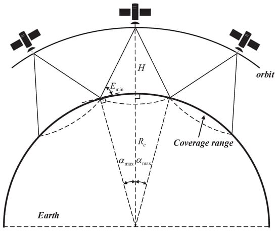
Figure 1. Satellite coverage geometry.

The coverage range of adjacent coplanar satellites overlaps with each other, forming a street-of-coverage (SOC), shown in Figure 2. The width of the SOC $\sigma$ depends on the coverage range ${\alpha }_{max}$ and the geocentric angle between adjacent coplanar satellites $\theta$, written in Equation (2).

$$\sigma =arccos\left({\displaystyle \frac{cos2{\alpha }_{max}}{cos\theta }}\right)$$

(2)

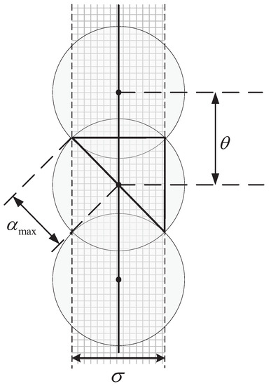
Figure 2. Street-of-coverage geometry of one orbital plane.

Since mega Walker constellation satellites are located at the same inclination, the SOC of adjacent orbital planes are approximately parallel to each other at low latitudes, shown in Figure 3. If the SOC of adjacent orbital planes could overlap with each other, continuous coverage can be achieved at low latitudes. It is noted that adjacent orbital planes could be co-rotating planes or counter-rotating planes, where satellites in the co-rotating planes move in the same direction ($\Delta \mathsf{\Omega }$ is close to zero), while satellites in the counter-rotating planes move in the opposite direction ($\Delta \mathsf{\Omega }$ is close to $\pi$). Therefore, the relative motion relationships between co-rotating satellites are relatively fixed compared to counter-rotating satellites. From the perspective of self-organization, the adjacent orbital planes in the coverage constraint are specified as co-rotating planes.

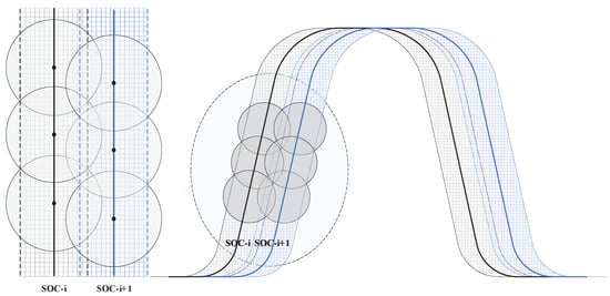
Figure 3. Streets-of-coverage geometries of adjacent orbital planes.

To sum up, the continuous coverage constraint of the mega constellation is defined as follows: The continuous coverage can be guaranteed for a designed latitude range if the SOC of every two adjacent co-rotating orbital planes overlaps with each other. Theoretically, the existence of adjacent counter-rotating orbital planes can provide more coverage multiplicity.

2.1.2. Configuration Requirements for Mega Constellations

The mega constellation, containing a total of N satellites, is composed of S satellites evenly spaced on each of P orbital plane. The geocentric angle between adjacent coplanar satellites $\theta$ is $2\pi /S$. According to Equation (2), the width of SOC of one orbital plane $\sigma$ is

$$\sigma =arccos\left({\displaystyle \frac{cos2{\alpha }_{max}}{cos\left(2\pi /\phantom{2\pi S}S\right)}}\right)$$

(3)

where

$$S\ge \pi /\phantom{\pi {\alpha }_{max}}{\alpha }_{max}$$

(4)

To ensure the SOC of every two adjacent co-rotating orbital planes overlaps with each other there exists

$$\sigma \ge 2\pi /\phantom{2\pi P}P$$

(5)

From Equations (3) and (5), it can be implied that

$$cos\left({\displaystyle \frac{2\pi }{P}}\right)cos\left({\displaystyle \frac{2\pi }{S}}\right)\ge cos\left(2{\alpha }_{max}\right)$$

(6)

Therefore, the configuration requirements for mega constellations that satisfy the proposed continuous coverage constraint are given in Equations (4) and (6).

Several ongoing and planned mega constellation missions are listed in Table 1. Let the minimum elevation angle $E_{min}$ takes 20${}^{\circ }$. The coverage range ${\alpha }_{\max }$ can be calculated by Equation (1) together with the orbital altitude. Most of these mega constellations are proven to satisfy the configuration requirements for continuous coverage, i.e., Equations (4) and (6).

Table 1. Summary of several mega constellation missions.

Constellation	Altitude	Inclination	Planes	Satellites per Plane	Whether Continuous Coverage Constraint Is Satisfied
Starlink Genaration 1	550 km	53${}^{\circ }$	72	22	Yes
	540 km	53.2${}^{\circ }$	72	22	Yes
	570 km	70${}^{\circ }$	36	20	Yes
	560 km	97.6${}^{\circ }$	6	58	No
	560 km	97.6${}^{\circ }$	4	43	No
OneWeb	1120 km	87.9${}^{\circ }$	18	40	Yes
	1150 km	53${}^{\circ }$	32	50	Yes
	1110 km	53.8${}^{\circ }$	32	50	Yes
GW-A59	590 km	85${}^{\circ }$	16	30	No
	600 km	50${}^{\circ }$	40	50	Yes
	508 km	55${}^{\circ }$	60	60	Yes
GW-2	1145 km	30${}^{\circ }$	48	36	Yes
	1145 km	40${}^{\circ }$	48	36	Yes
	1145 km	50${}^{\circ }$	48	36	Yes
	1145 km	60${}^{\circ }$	48	36	Yes

2.1.3. Intersatellite Motion Constraints

Due to perturbations and initial orbit errors, the coplanar satellites will drift from each other, and thus the RAAN differences between coplanar satellites will get larger over time without consideration of constellation control. The drift range of the RAAN difference between adjacent co-rotating orbital planes $\delta \mathsf{\Omega }$, and the drift range of the geocentric angle between adjacent coplanar satellites $\theta$ under the continuous coverage constraint, are worth investigating.

The SOC geometry of the perturbed coplanar satellites is shown in Figure 4, where

$$\angle \mathrm{AC}=arccos\left({\displaystyle \frac{cos2{\alpha }_{max}}{cos\theta }}\right)$$

(7)

$$\angle \mathrm{DE}=\theta$$

(8)

$$\angle \mathrm{EF}=\delta \mathsf{\Omega }$$

(9)

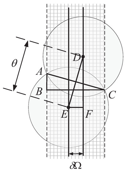
Figure 4. Street-of-coverage geometry of the perturbed coplanar satellites. D and E are two sub-satellite points. A and C are two intersections of two coverage circle. Point A, B, C form a right triangle. Point D, E, F form a right triangle.

It can be calculated that the coverage range of two adjacent coplanar satellites along the track direction is

$$\angle \mathrm{DF}=arccos\left({\displaystyle \frac{cos\theta }{cos\delta \mathsf{\Omega }}}\right)$$

(10)

The coverage range along the normal direction of the orbital plane is

$$\angle \mathrm{BC}={\displaystyle \frac{sin\theta cos2{\alpha }_{max}}{\sqrt{{sin}^2\theta {cos}^2\theta -\left({cos}^2\theta -{cos}^{2}2{\alpha }_{max}\right){sin}^2\delta \mathsf{\Omega }}}}$$

(11)

To ensure the SOC of every two adjacent co-rotating orbital planes overlap with each other, there exists

$$\angle \mathrm{BC}\ge {\displaystyle \frac{2\pi }{P}}$$

(12)

To ensure the coverage range of every two adjacent coplanar satellites along the track direction overlap with each other, there exists

$$\angle \mathrm{D}{\mathrm{F}}_{max}\ge {\displaystyle \frac{2\pi }{S}}$$

(13)

According to Equations (11) and (12), the drift range of $\theta$ can be obtained, which is related to the drift range of $\delta \mathsf{\Omega }$.

$${\theta }_{min}\le \theta \le {\theta }_{max}$$

(14)

where

$$\begin{array}{c}{A}_1=-{cos}^2\left({\displaystyle \frac{2\pi }{P}}\right)\hfill \\ B_1=-{cos}^2\left({\displaystyle \frac{2\pi }{P}}\right)\left(1+{sin}^2\delta \mathsf{\Omega }\right)+{cos}^{2}2{\alpha }_{max}\hfill \\ C_1={cos}^2\left({\displaystyle \frac{2\pi }{P}}\right){sin}^{2}2{\alpha }_{max}{sin}^2\delta \mathsf{\Omega }\hfill \\ {\theta }_{min}=arcsin\left(\sqrt{{\displaystyle \frac{-B_1-\sqrt{B_1^2-4A_1{C}_1}}{2A_1}}}\right)\hfill \\ {\theta }_{max}=arcsin\left(\sqrt{{\displaystyle \frac{-B_1+\sqrt{B_1^2-4A_1{C}_1}}{2A_1}}}\right)\hfill \end{array}$$

(15)

According to Equations (10), (13) and (14), the drift range of $\delta \mathsf{\Omega }$ of every two adjacent satellites can be obtained as

$$0\le \delta \mathsf{\Omega }\le arcsin\left(\sqrt{{\displaystyle \frac{B_2}{A_2}}}\right)$$

(16)

where

$$\begin{array}{c}{A}_2=-2{sin}^2\left({\displaystyle \frac{2\pi }{S}}\right){cos}^2\left({\displaystyle \frac{2\pi }{S}}\right){cos}^2\left({\displaystyle \frac{2\pi }{P}}\right)-{cos}^2\left({\displaystyle \frac{2\pi }{S}}\right){cos}^{2}2{\alpha }_{max}+{cos}^2\left({\displaystyle \frac{2\pi }{P}}\right){cos}^{2}2{\alpha }_{max}\hfill \\ B_2=-{sin}^2\left({\displaystyle \frac{2\pi }{S}}\right)\left[{cos}^2\left({\displaystyle \frac{2\pi }{S}}\right){cos}^2\left({\displaystyle \frac{2\pi }{P}}\right)-{cos}^{2}2{\alpha }_{max}\right]\hfill \end{array}$$

(17)

The detailed derivation steps and the proofs of real roots are given in Appendix A.

We denote $\mathsf{\Omega }{}_t$ as the target RAAN under $J_2$ perturbation of the designed orbital plane. Then the drift range of ${\mathsf{\Omega }}_i$ of all coplanar satellites away from $\mathsf{\Omega }{}_t$ can be written as

$$\begin{array}{c}\delta {\mathsf{\Omega }}_i={\mathsf{\Omega }}_i-{\mathsf{\Omega }}_t\ge -{\displaystyle \frac{1}{2}}arcsin\left(\sqrt{{\displaystyle \frac{B_2}{A_2}}}\right)=\delta {\mathsf{\Omega }}_{min}\hfill \\ \delta {\mathsf{\Omega }}_i={\mathsf{\Omega }}_i-{\mathsf{\Omega }}_t\le {\displaystyle \frac{1}{2}}arcsin\left(\sqrt{{\displaystyle \frac{B_2}{A_2}}}\right)=\delta {\mathsf{\Omega }}_{max}\hfill \end{array}$$

(18)

We denote the position vectors of two adjacent coplanar satellites in the geocentric inertial frame as ${\mathbf{r}}_i$ and ${\mathbf{r}}_{i+1}$. The constraint of $\theta$ can be transformed to the relative distance constraint $d_{i,i+1}$ by means of cosine theorem.

$$\begin{array}{c}{d}_{i,i+1}\ge \sqrt{{∥{\mathbf{r}}_i∥}^2+{∥{\mathbf{r}}_{i+1}∥}^2-2∥{\mathbf{r}}_i∥∥{\mathbf{r}}_{i+1}∥cos{\theta }_{min}}\hfill \\ d_{i,i+1}\le \sqrt{{∥{\mathbf{r}}_i∥}^2+{∥{\mathbf{r}}_{i+1}∥}^2-2∥{\mathbf{r}}_i∥∥{\mathbf{r}}_{i+1}∥cos{\theta }_{max}}\hfill \end{array}$$

(19)

Considering that mega constellations are nearly circular orbits, the position vectors in the geocentric inertial frame are substituted by semi-major axis a, given in Equation (20).

$$\begin{array}{c}{d}_{i,i+1}\ge \sqrt{2a^2\left(1-cos{\theta }_{min}\right)}=d_{\mathrm{mint}}\hfill \\ d_{i,i+1}\le \sqrt{2a^2\left(1-cos{\theta }_{max}\right)}=d_{\mathrm{maxt}}\hfill \end{array}$$

(20)

To sum up, the intersatellite motion constraints that every two adjacent coplanar satellites should obey during their lifetime are presented in Equations (18) and (20).

2.2. Self-Organizing Control Using Artificial Potential Functions

In this section, the scale-independent relative orbital elements (SIROEs), as well as the corresponding bound formulations, are introduced first. The relative motion bound denotes the maximum or minimum value of the relative distance between two satellites. Based on SIROEs, the artificial potential functions for single satellite control are designed under the continuous coverage constraint. The self-organizing control rules for the coplanar satellites are presented.

2.2.1. Scale-Independent Relative Orbital Elements and Bound Formulations

Scale-independent relative orbital elements are high-precision configuration parameters for relative motion with near-circular reference orbit and arbitrary intersatellite separation. SIROEs have been proposed in our preliminary work [23]. Six independent SIROEs are $b_1,b_2,b_3,c,{\theta }_1,{\theta }_2$, shown in Figure 5 and Figure 6. The relationship between SIROEs and relative position is given in Equation (21). We denote $\tilde{x},\tilde{y},\tilde{z}$ as the basic relative motion coordinates. The relative trajectory can be obtained by rotating the basic trajectory by ${\theta }_1$, counterclockwise. The basic trajectory projected on the $x-y$ plane is the combination of an ellipse (with a semi-major axis of $2b_1$ and a semi-minor axis of $b_1$), a circle (with a radius of $b_2$), and an additional offset (with x-offset of $b_3-acos{\theta }_1$ and y-offset of $asin{\theta }_1$). The relative motion on the z-axis is harmonic.

$$\begin{array}{cc}\left[\begin{array}{c}x\\ y\\ z\end{array}\right]\hfill & =\left[\begin{array}{ccc}cos{\theta }_1& -sin{\theta }_1& 0\\ sin{\theta }_1& cos{\theta }_1& 0\\ 0& 0& 1\end{array}\right]\left[\begin{array}{c}-b_{1}cos\left({\theta }_2+\psi \right)+b_{2}cos2\psi +b_3-acos{\theta }_1\\ 2b_{1}sin\left({\theta }_2+\psi \right)-b_{2}sin2\psi +asin{\theta }_1\\ csin\psi \end{array}\right]\hfill \\ \hfill & =\left[\begin{array}{ccc}cos{\theta }_1& -sin{\theta }_1& 0\\ sin{\theta }_1& cos{\theta }_1& 0\\ 0& 0& 1\end{array}\right]\left[\begin{array}{c}\tilde{x}\\ \tilde{y}\\ \tilde{z}\end{array}\right]\hfill \end{array}$$

(21)

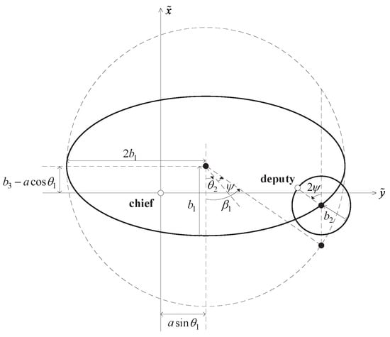
Figure 5. Illustration of the scale-independent relative orbital elements ($x-y$ plane).

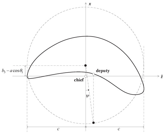
Figure 6. Illustration of the scale-independent relative orbital elements ($x-z$ plane).

Without regard to the minor differences of semi-major axes between constellation satellites, the relative velocities represented by SIROEs are written as

$$\left[\begin{array}{c}\dot{x}/\phantom{\dot{x}n}n\\ \dot{y}/\phantom{\dot{y}n}n\\ \dot{z}/\phantom{\dot{z}n}n\end{array}\right]=\left[\begin{array}{ccc}cos{\theta }_1& -sin{\theta }_1& 0\\ sin{\theta }_1& cos{\theta }_1& 0\\ 0& 0& 1\end{array}\right]\left[\begin{array}{c}{b}_{1}sin\left({\theta }_2+\psi \right)-2b_{2}sin2\psi \\ 2b_{1}cos\left({\theta }_2+\psi \right)-2b_{2}cos2\psi \\ ccos\psi \end{array}\right]$$

(22)

where n is the mean angular velocity of the reference orbit.

According to Equations (21) and (22), SIROEs can be represented by translational states, given in Equation (23).

$$\begin{array}{c}c=\sqrt{z^2+{\left(\dot{z}/\phantom{\dot{z}n}n\right)}^2}\hfill \\ sin\psi =z/\phantom{zc}c,cos\psi =\dot{z}/\phantom{\dot{z}nc}nc\hfill \\ b_2={\displaystyle \frac{1}{2}}\left(a^{\prime }-\sqrt{a{}^{\prime 2}-c^2}\right)\hfill \\ b_3={\displaystyle \frac{1}{2}}\left(a^{\prime }+\sqrt{a{}^{\prime 2}-c^2}\right)\hfill \\ cos{\theta }_1=-{\displaystyle \frac{2b_3\left(2\dot{y}+nx+na\right)+3b_{2}sin2\psi \left(2ny-\dot{x}\right)}{\left(2\dot{x}-ny\right)\left(2ny-\dot{x}\right)-\left(2nx+2na+\dot{y}\right)\left(2\dot{y}+nx+na\right)}}\hfill \\ sin{\theta }_1={\displaystyle \frac{2n{b}_3-\left(2nx+2na+\dot{y}\right)cos{\theta }_1}{2ny-\dot{x}}}\hfill \\ b_1=\sqrt{{\left[-\left(x+a\right)cos{\theta }_1-ysin{\theta }_1+b_{2}cos2\psi +b_3\right]}^2+{\left({\displaystyle \frac{\dot{x}}{n}}cos{\theta }_1+\frac{\dot{y}}{n}sin{\theta }_1+2b_{2}sin2\psi \right)}^2}\hfill \\ sin{\beta }_1={\displaystyle \frac{\dot{x}cos{\theta }_1+\dot{y}sin{\theta }_1+2n{b}_{2}sin2\psi }{n{b}_1}}\hfill \\ cos{\beta }_1={\displaystyle \frac{-\left(x+a\right)cos{\theta }_1-ysin{\theta }_1+b_{2}cos2\psi +b_3}{b_1}}\hfill \\ sin{\theta }_2=sin{\beta }_{1}cos\psi -cos{\beta }_{1}sin\psi \hfill \\ cos{\theta }_2=cos{\beta }_{1}cos\psi +sin{\beta }_{1}sin\psi \hfill \end{array}$$

(23)

According to Equation (21), the squared relative distance between satellites can be written as

$$w=x^2+y^2+z^2={\displaystyle \frac{A_3{s}^6+B_3{s}^5+C_3{s}^4+D_3{s}^3+E_3{s}^2+F_{3}s+G_3}{{\left(1+s^2\right)}^3}}$$

(24)

where

$$s=tan{\displaystyle \frac{\psi }{2}},\begin{array}{cc}& \psi \in \left[0,2\pi \right)\end{array}$$

(25)

Parameters $A_3,B_3,C_3,D_3,E_3,F_3,G_3$ are polynomials about SIROEs $b_1,b_2,b_3,c,{\theta }_1,{\theta }_2$. Therefore, $A_3,B_3,C_3,D_3,E_3,F_3,G_3$ are time-invariant, while s is the only time variable. Differentiating w with respect to s results in

$$\frac{\partial w}{\partial s}=\frac{\begin{array}{c}-B_3{s}^6+\left(6A_3-2C_3\right)s^5+\left(5B_3-3D_3\right)s^4+\left(4C_3-4E_3\right)s^3+\left(3D_3-5F_3\right)s^2\hfill \\ +\left(2E_3-6G_3\right)s^3+F_3\hfill \end{array}}{{\left(1+s^2\right)}^4}$$

(26)

Let $\partial w/\phantom{\partial w\partial s}\partial s=0$, there exists

$$\begin{array}{c}-B_3{s}^6+\left(6A_3-2C_3\right)s^5+\left(5B_3-3D_3\right)s^4+\left(4C_3-4E_3\right)s^3+\left(3D_3-5F_3\right)s^2\hfill \\ +\left(2E_3-6G_3\right)s^3+F_3=0\hfill \end{array}$$

(27)

or

$$s=\pm \infty$$

(28)

The real roots of Equation (27) together with $s=\pm \infty$ constitute a set of s values that perhaps make the squared relative distance take the maximum or minimum value, which are relative motion bounds. Note that when $s=\pm \infty$, $\psi =\pm \pi$, the squared relative distance takes $w=A_3$.

Assuming that $s_{max}$ is the s value that makes the squared relative distance w take the maximum value and $s_{min}$ is the one that makes w take the minimum value, the maximum bound ${\stackrel{⌢}{d}}_{ij}$ and the minimum bound ${\stackrel{⌣}{d}}_{ij}$ for the current time can be written as

$$\left\{\begin{array}{c}{\stackrel{⌢}{d}}_{ij}=\sqrt{{\displaystyle \frac{A_3{s}_{max}^6+B_3{s}_{max}^5+C_3{s}_{max}^4+D_3{s}_{max}^3+E_3{s}_{max}^2+F_3{s}_{max}+G_3}{{\left(1+s_{max}^2\right)}^3}}},\mathrm{if}{s}_{max}\ne \pm \infty \hfill \\ {\stackrel{⌢}{d}}_{ij}=\sqrt{A_3},\mathrm{if}{s}_{max}=\pm \infty \hfill \end{array}\right.$$

(29)

$$\left\{\begin{array}{c}{\stackrel{⌣}{d}}_{ij}=\sqrt{{\displaystyle \frac{A_3{s}_{min}^6+B_3{s}_{min}^5+C_3{s}_{min}^4+D_3{s}_{min}^3+E_3{s}_{min}^2+F_3{s}_{min}+G_3}{{\left(1+s_{min}^2\right)}^3}}},\mathrm{if}{s}_{min}\ne \pm \infty \hfill \\ {\stackrel{⌣}{d}}_{ij}=\sqrt{A_3},\mathrm{if}{s}_{min}=\pm \infty \hfill \end{array}\right.$$

(30)

Relative motion bounds are complicated functions of SIROEs, and SIROEs are functions about translational states, given in Equation (23). Therefore, ${\stackrel{⌢}{d}}_{ij}$ and ${\stackrel{⌣}{d}}_{ij}$ are functions about translational states $x,y,z,\dot{x},\dot{y},\dot{z}$.

2.2.2. Design of Artificial Potential Functions for Single Satellite Control

Referring to the concept of relative motion bound, Equation (20) can be rewritten as ${\stackrel{⌢}{d}}_{ij}\le d_{\mathrm{maxt}}$, ${\stackrel{⌣}{d}}_{ij}\ge d_{\mathrm{mint}}$. Together with Equation (18), the proposed continuous coverage constraint relates to RAAN differences and relative motion bounds. Therefore, the control effects will be performed in cases if $\delta {\mathsf{\Omega }}_i>\delta {\mathsf{\Omega }}_{max}$ or $\delta {\mathsf{\Omega }}_i<\delta {\mathsf{\Omega }}_{min}$ or ${\stackrel{⌢}{d}}_{ij}>d_{\mathrm{maxt}}$ or ${\stackrel{⌣}{d}}_{ij}<d_{\mathrm{mint}}$.

The following artificial potential functions are all designed in quadratic form, given in Equation (31).

$${\varphi }_i={\left({\mathbf{X}}_i-{\mathbf{X}}_{\mathrm{t}}\right)}^{\mathrm{T}}\mathbf{K}\left({\mathbf{X}}_i-{\mathbf{X}}_{\mathrm{t}}\right)$$

(31)

where ${\mathbf{X}}_i$ is the control variable. ${\mathbf{X}}_{\mathrm{t}}$ is the expected value of ${\mathbf{X}}_i$. $\mathbf{K}$ is the control coefficient matrix, which is a positive definite symmetric matrix. In the geocentric inertial frame, the control effect generated from ${\varphi }_i$ is given as

$$\Delta {\mathbf{V}}_i=-{\displaystyle \frac{\partial {\mathbf{X}}_i^T}{\partial {\mathbf{V}}_i}}{\displaystyle \frac{\partial {\varphi }_i}{\partial {\mathbf{X}}_i}}=-\left[\begin{array}{c}{\displaystyle \frac{\partial {\mathbf{X}}_i^T}{\partial \dot{X}}}{\displaystyle \frac{\partial {\varphi }_i}{\partial {\mathbf{X}}_i}}\\ {\displaystyle \frac{\partial {\mathbf{X}}_i^T}{\partial \dot{Y}}}{\displaystyle \frac{\partial {\varphi }_i}{\partial {\mathbf{X}}_i}}\\ {\displaystyle \frac{\partial {\mathbf{X}}_i^T}{\partial \dot{Z}}}{\displaystyle \frac{\partial {\varphi }_i}{\partial {\mathbf{X}}_i}}\end{array}\right]$$

(32)

where ${\mathbf{V}}_i={\left[\dot{X},\dot{Y},\dot{Z}\right]}^{\mathrm{T}}$ represents the geocentric velocity vector of satellite i. Hence, the velocity increments of ${\varphi }_i$ are the negative gradient of ${\varphi }_i$ with respect to satellite i’s geocentric velocity vector ${\mathbf{V}}_i$. The stability proof will be given in Section 4.

(1)

RAAN Control

To limit the RAAN difference, the artificial potential function is designed in Equation (33). The control variable takes ${\mathbf{X}}_i={\left[sin{i}_{i}sin{\mathsf{\Omega }}_i,sin{i}_{i}cos{\mathsf{\Omega }}_i\right]}^{\mathrm{T}}$. The control coefficient matrix takes $\mathbf{K}=\mathrm{diag}\left(k_{i\mathsf{\Omega }},k_{i\mathsf{\Omega }}\right)$. $\delta {\mathsf{\Omega }}_i={\mathsf{\Omega }}_i-{\mathsf{\Omega }}_t$. $i_t$ and ${\mathsf{\Omega }}_t$ represent the target inclination and RAAN values under $J_2$ perturbation of the designed orbital plane, respectively. Therefore, ${\varphi }_{i\mathsf{\Omega }}$ limits the RAAN difference within the expected range and corrects the inclination meanwhile.

$${\varphi }_{i,i\mathsf{\Omega }}=\left\{\begin{array}{c}{k}_{i\mathsf{\Omega }}{\left(sin{i}_{i}sin{\mathsf{\Omega }}_i-sin{i}_{t}sin{\mathsf{\Omega }}_t\right)}^2+k_{i\mathsf{\Omega }}{\left(sin{i}_{i}cos{\mathsf{\Omega }}_i-sin{i}_{t}cos{\mathsf{\Omega }}_t\right)}^2,\hfill \\ \mathrm{if}\delta {\mathsf{\Omega }}_i>\delta {\mathsf{\Omega }}_{max}\cup \delta {\mathsf{\Omega }}_i<\delta {\mathsf{\Omega }}_{min}\hfill \\ 0,\mathrm{if}\delta {\mathsf{\Omega }}_{min}\le \delta {\mathsf{\Omega }}_i\le \delta {\mathsf{\Omega }}_{max}\hfill \end{array}\right.$$

(33)

According to Equation (32), the velocity increments generated by ${\varphi }_{i,i\mathsf{\Omega }}$ in the geocentric inertial frame are

$$\begin{array}{c}\Delta {\mathbf{V}}_{i,i\mathsf{\Omega }}=-{\displaystyle \frac{\partial {\mathbf{X}}_i^{\mathrm{T}}}{\partial {\mathbf{V}}_i}}{\displaystyle \frac{\partial {\varphi }_{i,i\mathsf{\Omega }}}{\partial {\mathbf{X}}_i}}\hfill \\ =-\left[\begin{array}{c}{\displaystyle \frac{\partial {\varphi }_{i,i\mathsf{\Omega }}}{\partial sin{i}_{i}sin{\mathsf{\Omega }}_i}}{\displaystyle \frac{\partial sin{i}_{i}sin{\mathsf{\Omega }}_i}{\partial \dot{X}}}+{\displaystyle \frac{\partial {\varphi }_{i,i\mathsf{\Omega }}}{\partial sin{i}_{i}cos{\mathsf{\Omega }}_i}}{\displaystyle \frac{\partial sin{i}_{i}cos{\mathsf{\Omega }}_i}{\partial \dot{X}}}\\ {\displaystyle \frac{\partial {\varphi }_{i,i\mathsf{\Omega }}}{\partial sin{i}_{i}sin{\mathsf{\Omega }}_i}}{\displaystyle \frac{\partial sin{i}_{i}sin{\mathsf{\Omega }}_i}{\partial \dot{Y}}}+{\displaystyle \frac{\partial {\varphi }_{i,i\mathsf{\Omega }}}{\partial sin{i}_{i}cos{\mathsf{\Omega }}_i}}{\displaystyle \frac{\partial sin{i}_{i}cos{\mathsf{\Omega }}_i}{\partial \dot{Y}}}\\ {\displaystyle \frac{\partial {\varphi }_{i,i\mathsf{\Omega }}}{\partial sin{i}_{i}sin{\mathsf{\Omega }}_i}}{\displaystyle \frac{\partial sin{i}_{i}sin{\mathsf{\Omega }}_i}{\partial \dot{Z}}}+{\displaystyle \frac{\partial {\varphi }_{i,i\mathsf{\Omega }}}{\partial sin{i}_{i}cos{\mathsf{\Omega }}_i}}{\displaystyle \frac{\partial sin{i}_{i}cos{\mathsf{\Omega }}_i}{\partial \dot{Z}}}\end{array}\right]\hfill \end{array}$$

(34)

The relationship between ${\mathbf{X}}_i$ and ${\mathbf{V}}_i$ is given as

$$\begin{array}{c}sin{i}_{i}sin{\mathsf{\Omega }}_i=\frac{Y\dot{Z}-Z\dot{Y}}{\sqrt{{\left(Y\dot{Z}-Z\dot{Y}\right)}^2+{\left(Z\dot{X}-X\dot{Z}\right)}^2+{\left(X\dot{Y}-Y\dot{X}\right)}^2}}\hfill \\ sin{i}_{i}cos{\mathsf{\Omega }}_i=\frac{-\left(Z\dot{X}-X\dot{Z}\right)}{\sqrt{{\left(Y\dot{Z}-Z\dot{Y}\right)}^2+{\left(Z\dot{X}-X\dot{Z}\right)}^2+{\left(X\dot{Y}-Y\dot{X}\right)}^2}}\hfill \end{array}$$

(35)

In fact, the out-of-plane control can be avoided by setting an appropriate offset of the semi-major axis to ensure the time derivative of $\mathsf{\Omega }$ is approximately zero under perturbations. Take the GW-2 constellation, for instance. The drift range of $\delta \mathsf{\Omega }$ is $\pm {12.14}^{\circ }$ when $E_{min}={20}^{\circ }$ according to Equation (18). The drift range of $\delta \mathsf{\Omega }$ is relatively large, where the RAAN control will basically not be implemented in two years.

(2)

Relative Motion-bound Control

To realize the restriction of relative motion bound, the artificial potential function is designed in Equation (36). The control variable takes ${\mathbf{X}}_i={\stackrel{⌣}{d}}_{ij}$ or ${\mathbf{X}}_i={\stackrel{⌢}{d}}_{ij}$, and the control coefficient matrix takes the $\mathbf{K}=k_{bound}$.

$${\varphi }_{i,bound}=\left\{\begin{array}{c}{k}_{bound}{\left({\stackrel{⌣}{d}}_{ij}-d_{\mathrm{mint}}\right)}^2,\mathrm{if}{\stackrel{⌣}{d}}_{ij}<d_{\mathrm{mint}}\hfill \\ k_{bound}{\left({\stackrel{⌢}{d}}_{ij}-d_{\mathrm{maxt}}\right)}^2,\mathrm{if}{\stackrel{⌢}{d}}_{ij}>d_{\mathrm{maxt}}\hfill \\ 0,\mathrm{if}{\stackrel{⌣}{d}}_{ij}\ge d_{\mathrm{mint}}\cap {\stackrel{⌢}{d}}_{ij}\le d_{\mathrm{maxt}}\hfill \end{array}\right.$$

(36)

Satellite j is designated as the reference satellite. $d_{\mathrm{mint}}$ and $d_{\mathrm{maxt}}$ are determined by Equation (20).

In the geocentric inertial frame, the velocity increments generated by ${\varphi }_{i,bound}$ can be obtained by calculating the negative gradient of ${\varphi }_{i,bound}$ with respect to the relative velocity vector ${\mathbf{v}}_i={\left[\dot{x},\dot{y},\dot{z}\right]}^{\mathrm{T}}$, and then transforming them from satellite j’s orbital frame to the geocentric inertial frame.

$$\Delta {\mathbf{V}}_{i,bound}=-{\mathbf{Q}}_j^{-1}{\displaystyle \frac{\partial {\mathbf{X}}_i^{\mathrm{T}}}{\partial {\mathbf{v}}_i}}{\displaystyle \frac{\partial {\varphi }_{i,bound}}{\partial {\mathbf{X}}_i}}=-{\mathbf{Q}}_j^{-1}\left[\begin{array}{c}{\displaystyle \frac{\partial {\varphi }_{i,bound}}{\partial {\stackrel{⌢}{d}}_{ij}}}{\displaystyle \frac{\partial {\stackrel{⌢}{d}}_{ij}}{\partial \dot{x}}}+{\displaystyle \frac{\partial {\varphi }_{i,bound}}{\partial {\stackrel{⌣}{d}}_{ij}}}{\displaystyle \frac{\partial {\stackrel{⌣}{d}}_{ij}}{\partial \dot{x}}}\\ {\displaystyle \frac{\partial {\varphi }_{i,bound}}{\partial {\stackrel{⌢}{d}}_{ij}}}{\displaystyle \frac{\partial {\stackrel{⌢}{d}}_{ij}}{\partial \dot{y}}}+{\displaystyle \frac{\partial {\varphi }_{i,bound}}{\partial {\stackrel{⌣}{d}}_{ij}}}{\displaystyle \frac{\partial {\stackrel{⌣}{d}}_{ij}}{\partial \dot{y}}}\\ {\displaystyle \frac{\partial {\varphi }_{i,bound}}{\partial {\stackrel{⌢}{d}}_{ij}}}{\displaystyle \frac{\partial {\stackrel{⌢}{d}}_{ij}}{\partial \dot{z}}}+{\displaystyle \frac{\partial {\varphi }_{i,bound}}{\partial {\stackrel{⌣}{d}}_{ij}}}{\displaystyle \frac{\partial {\stackrel{⌣}{d}}_{ij}}{\partial \dot{z}}}\end{array}\right]$$

(37)

$\partial \left({\stackrel{⌢}{d}}_{ij},{\stackrel{⌣}{d}}_{ij}\right)/\phantom{\partial \left({\stackrel{⌢}{d}}_{ij},{\stackrel{⌣}{d}}_{ij}\right)\partial \dot{x}}\partial \dot{x}$, $\partial \left({\stackrel{⌢}{d}}_{ij},{\stackrel{⌣}{d}}_{ij}\right)/\phantom{\partial \left({\stackrel{⌢}{d}}_{ij},{\stackrel{⌣}{d}}_{ij}\right)\partial \dot{y}}\partial \dot{y}$, $\partial \left({\stackrel{⌢}{d}}_{ij},{\stackrel{⌣}{d}}_{ij}\right)/\phantom{\partial \left({\stackrel{⌢}{d}}_{ij},{\stackrel{⌣}{d}}_{ij}\right)\partial \dot{z}}\partial \dot{z}$ can be formulated based on Equations (23), (24), (29) and (30). ${\mathbf{Q}}_j$ represents the transformation matrix from the geocentric inertial frame to satellite j’s orbital frame.

$${\mathbf{Q}}_j=\left[\begin{array}{ccc}-sin{\mathsf{\Omega }}_{j}cos{i}_j{\mathrm{sinu}}_j+cos{\mathsf{\Omega }}_j{\mathrm{cosu}}_j& cos{\mathsf{\Omega }}_{j}cos{i}_j{\mathrm{sinu}}_j+sin{\mathsf{\Omega }}_j{\mathrm{cosu}}_j& sin{i}_j{\mathrm{sinu}}_j\\ -sin{\mathsf{\Omega }}_{j}cos{i}_j{\mathrm{cosu}}_j-cos{\mathsf{\Omega }}_j{\mathrm{sinu}}_j& cos{\mathsf{\Omega }}_{j}cos{i}_j{\mathrm{cosu}}_j-sin{\mathsf{\Omega }}_j{\mathrm{sinu}}_j& sin{i}_j{\mathrm{cosu}}_j\\ sin{\mathsf{\Omega }}_{j}sin{i}_j& -cos{\mathsf{\Omega }}_{j}sin{i}_j& cos{i}_j\end{array}\right]$$

(38)

(3)

Semi-Major Axis Control

The differences in semi-major axes between constellation satellites will lead to secular drift, and hence the relative motion-bound constraint will never be satisfied. Moreover, the semi-major axis will keep declining because of the influence of atmospheric drag. From this perspective, semi-major axis control is essential to mega constellation maintenance.

The artificial potential function is designed to be a quadratic function about $a_i$, given in Equation (39). ${\mathbf{X}}_i=a_i$. $\mathbf{K}=k_a$. $a_t$ is the designed value of the orbital semi-major axis. Semi-major axis control will be implemented when the continuous coverage constraint has been satisfied.

$${\varphi }_{i,a}=\left\{\begin{array}{c}{k}_a{\left(a_i-a_t\right)}^2,\mathrm{if}{\stackrel{⌣}{d}}_{ij}\ge d_{\mathrm{mint}}\cap {\stackrel{⌢}{d}}_{ij}\le d_{\mathrm{maxt}}\cap \delta \mathsf{\Omega }\ge \delta {\mathsf{\Omega }}_{min}\cap \delta \mathsf{\Omega }\le \delta {\mathsf{\Omega }}_{max}\hfill \\ 0,\mathrm{if}{\stackrel{⌣}{d}}_{ij}<d_{\mathrm{mint}}\cup {\stackrel{⌢}{d}}_{ij}>d_{\mathrm{maxt}}\cup \delta \mathsf{\Omega }<\delta {\mathsf{\Omega }}_{min}\cup \delta \mathsf{\Omega }>\delta {\mathsf{\Omega }}_{max}\hfill \end{array}\right.$$

(39)

The velocity increment of ${\varphi }_{i,a}$ in the geocentric inertial frame is

$$\Delta {\mathbf{V}}_{i,a}=-{\displaystyle \frac{\partial {\mathbf{X}}_i^{\mathrm{T}}}{\partial {\mathbf{V}}_i}}{\displaystyle \frac{\partial {\varphi }_{i,a}}{\partial {\mathbf{X}}_i}}=-\left[\begin{array}{c}{\displaystyle \frac{\partial {\varphi }_{i,a}}{\partial a_i}}{\displaystyle \frac{\partial a_i}{\partial \dot{X}}}\\ {\displaystyle \frac{\partial {\varphi }_{i,a}}{\partial a_i}}{\displaystyle \frac{\partial a_i}{\partial \dot{Y}}}\\ {\displaystyle \frac{\partial {\varphi }_{i,a}}{\partial a_i}}{\displaystyle \frac{\partial a_i}{\partial \dot{Z}}}\end{array}\right]$$

(40)

The relationship between $a_i$ and ${\mathbf{V}}_i$ is given as

$$a_i=-\mu {\left[\left({\dot{X}}^2+{\dot{Y}}^2+{\dot{Z}}^2\right)-\frac{2\mu }{\sqrt{X^2+Y^2+Z^2}}\right]}^{-1}$$

(41)

To sum up, the control potential functions for satellite i are given as follows.

$${\varphi }_i=\left\{\begin{array}{c}{k}_{i\mathsf{\Omega }}{\left(sin{i}_{i}sin{\mathsf{\Omega }}_i-sin{i}_{t}sin{\mathsf{\Omega }}_t\right)}^2+k_{i\mathsf{\Omega }}{\left(sin{i}_{i}cos{\mathsf{\Omega }}_i-sin{i}_{t}cos{\mathsf{\Omega }}_t\right)}^2,\hfill \\ \mathrm{if}\delta \mathsf{\Omega }>\delta {\mathsf{\Omega }}_{max}\cup \delta \mathsf{\Omega }<\delta {\mathsf{\Omega }}_{min}\hfill \\ k_{bound}{\left({\stackrel{⌣}{d}}_{ij}-d_{\mathrm{mint}}\right)}^2,\mathrm{if}{\stackrel{⌣}{d}}_{ij}<d_{\mathrm{mint}}\hfill \\ k_{bound}{\left({\stackrel{⌢}{d}}_{ij}-d_{\mathrm{maxt}}\right)}^2,\mathrm{if}{\stackrel{⌢}{d}}_{ij}>d_{\mathrm{maxt}}\hfill \\ k_a{\left(a_i-a_t\right)}^2,\mathrm{if}\delta \mathsf{\Omega }\ge \delta {\mathsf{\Omega }}_{min}\cap \delta \mathsf{\Omega }\le \delta {\mathsf{\Omega }}_{max}\cap {\stackrel{⌣}{d}}_{ij}\ge d_{\mathrm{mint}}\cap {\stackrel{⌢}{d}}_{ij}\le d_{\mathrm{maxt}}\hfill \end{array}\right.$$

(42)

2.2.3. Self-Organizing Control Rules for Coplanar Satellites

For three adjacent coplanar satellites, $i-1$, i and $i+1$, the self-organizing control rules are defined as follows.

$${\varphi }_i=\left\{\begin{array}{c}{k}_{i\mathsf{\Omega }}{\left(sin{i}_{i}sin{\mathsf{\Omega }}_i-sin{i}_{t}sin{\mathsf{\Omega }}_t\right)}^2+k_{i\mathsf{\Omega }}{\left(sin{i}_{i}cos{\mathsf{\Omega }}_i-sin{i}_{t}cos{\mathsf{\Omega }}_t\right)}^2,\hfill \\ \mathrm{if}\delta \mathsf{\Omega }>\delta {\mathsf{\Omega }}_{max}\cup \delta \mathsf{\Omega }<\delta {\mathsf{\Omega }}_{min}\hfill \\ k_{bound}{\left({\stackrel{⌣}{d}}_{i,i-1}-d_{\mathrm{mint}}\right)}^2,\mathrm{if}{\stackrel{⌣}{d}}_{i,i-1}<d_{\mathrm{mint}}\cap {\stackrel{⌣}{d}}_{i,i+1}\ge d_{\mathrm{mint}}\hfill \\ k_{bound}{\left({\stackrel{⌣}{d}}_{i,i+1}-d_{\mathrm{mint}}\right)}^2,\mathrm{if}{\stackrel{⌣}{d}}_{i,i-1}\ge d_{\mathrm{mint}}\cap {\stackrel{⌣}{d}}_{i,i+1}<d_{\mathrm{mint}}\hfill \\ k_{bound}{\left({\stackrel{⌢}{d}}_{i,i-1}-d_{\mathrm{maxt}}\right)}^2,\mathrm{if}{\stackrel{⌢}{d}}_{i,i-1}>d_{\mathrm{maxt}}\cap {\stackrel{⌢}{d}}_{i,i+1}\le d_{\mathrm{maxt}}\hfill \\ k_{bound}{\left({\stackrel{⌢}{d}}_{i,i+1}-d_{\mathrm{maxt}}\right)}^2,\mathrm{if}{\stackrel{⌢}{d}}_{i,i-1}\le d_{\mathrm{maxt}}\cap {\stackrel{⌢}{d}}_{i,i+1}>d_{\mathrm{maxt}}\hfill \\ k_a{\left(a_i-a_t\right)}^2,\mathrm{else}\hfill \end{array}\right.$$

(43)

To put it simply, the RAAN control will be performed once the RAAN difference between satellite i and the designed value does not fit the $\delta \mathsf{\Omega }$ range. The relative motion-bound control will work only if one of two adjacent coplanar satellites of satellite i (denoted as $i-1$ and $i+1$) does not meet the boundary constraint while the other does. For other cases, the semi-major axis control will be implemented, even if ${\stackrel{⌢}{d}}_{i,i-1}$, ${\stackrel{⌣}{d}}_{i,i-1}$, ${\stackrel{⌢}{d}}_{i,i+1}$, and ${\stackrel{⌣}{d}}_{i,i+1}$ do not all meet the boundary constraint.

2.3. Stability Proof of Satellite Control

In this section, the stability of the proposed self-organizing control is proved based on the Gaussian equations and Lyapunov’s theory. The selection criteria of potential function variables for satellite control are discussed.

2.3.1. Stability Proof of RAAN Control and Semi-Major Axis Control

If there exists one Lyapunov function $\varphi$ that satisfies Equation (44), the control system can be proven to be stable.

$$\left\{\begin{array}{c}\varphi \left(\mathbf{0}\right)=0,\hfill \\ \varphi \left(\mathbf{X}\right)>0,\forall \mathbf{X}\ne \mathbf{0}\hfill \\ \dot{\varphi }\left(\mathbf{0}\right)=0,\hfill \\ \dot{\varphi }\left(\mathbf{X}\right)\le 0,\dot{\varphi }\left(\mathbf{X}\right)\not\equiv 0,\forall \mathbf{X}\ne \mathbf{0}\hfill \end{array}\right.$$

(44)

In this paper, ${\varphi }_i$ is designated as the Lyapunov function. Referring to Equation (31), it is obvious that ${\varphi }_i$ is positive definite. If the time derivative of ${\varphi }_i$ is negative definite, one can prove that the proposed APF control is stable.

For RAAN control and semi-major axis control, $\mathbf{X}={\mathbf{X}}_i-{\mathbf{X}}_{\mathrm{t}}=[sin{i}_{i}sin{\mathsf{\Omega }}_i-sin{i}_{\mathrm{t}}sin{\mathsf{\Omega }}_{\mathrm{t}},$$sin{i}_{i}cos{\mathsf{\Omega }}_i-sin{i}_{\mathrm{t}}cos{\mathsf{\Omega }}_{\mathrm{t}},a_i-a_{\mathrm{t}}{]}^{\mathrm{T}}$. Hence, $\mathbf{X}$ relates to controlled satellite i only.

According to Equation (31), the time derivative of ${\varphi }_i$ can be written as

$${\displaystyle \frac{\mathrm{d}{\varphi }_i}{\mathrm{d}t}}={\displaystyle \frac{\partial {\varphi }_i}{\partial {\mathbf{X}}_i^{\mathrm{T}}}}{\displaystyle \frac{\mathrm{d}{\mathbf{X}}_i^{\mathrm{T}}}{\mathrm{d}t}}+{\displaystyle \frac{\partial {\varphi }_i}{\partial {\mathbf{X}}_{\mathrm{t}}^{\mathrm{T}}}}{\displaystyle \frac{\mathrm{d}{\mathbf{X}}_{\mathrm{t}}^{\mathrm{T}}}{\mathrm{d}t}}$$

(45)

The time derivative of ${\mathbf{X}}_i$ is

$$\begin{array}{c}{\displaystyle \frac{\mathrm{d}{\mathbf{X}}_i}{\mathrm{d}t}}={\displaystyle \frac{\partial {\mathbf{X}}_i}{\partial {\mathbf{R}}_i^{\mathrm{T}}}}{\displaystyle \frac{\mathrm{d}{\mathbf{R}}_i}{\mathrm{d}t}}+{\displaystyle \frac{\partial {\mathbf{X}}_i}{\partial {\mathbf{V}}_i^{\mathrm{T}}}}{\displaystyle \frac{\mathrm{d}{\mathbf{V}}_i}{\mathrm{d}t}}\hfill \\ ={\displaystyle \frac{\partial {\mathbf{X}}_i}{\partial {\mathbf{R}}_i^{\mathrm{T}}}}{\displaystyle \frac{\mathrm{d}{\mathbf{R}}_i}{\mathrm{d}t}}+{\displaystyle \frac{\partial {\mathbf{X}}_i}{\partial {\mathbf{V}}_i^{\mathrm{T}}}}\left(-\mu {\displaystyle \frac{{\mathbf{R}}_i}{R_i^3}}+\mathbf{u}\right)\hfill \\ ={\left({\displaystyle \frac{\mathrm{d}{\mathbf{X}}_i}{\mathrm{d}t}}\right)}_{two-body}+{\displaystyle \frac{\partial {\mathbf{X}}_i}{\partial {\mathbf{V}}_i^{\mathrm{T}}}}\mathbf{u}\hfill \end{array}$$

(46)

where ${\mathbf{R}}_i$ and ${\mathbf{V}}_i$ are the position vector and velocity vector in the geocentric inertial frame, respectively. $\mathbf{u}$ represents the control acceleration vector in the geocentric inertial frame. ${\left(\mathrm{d}{\mathbf{X}}_i/\phantom{\mathrm{d}{\mathbf{X}}_i\mathrm{d}t}\mathrm{d}t\right)}_{two-body}$ represents the time derivative of ${\mathbf{X}}_i$ under the two-body Keplerian motion condition.

Since ${\mathbf{X}}_{\mathrm{t}}$ does not change under control, the time derivative of ${\mathbf{X}}_{\mathrm{t}}$ is

$${\displaystyle \frac{\mathrm{d}{\mathbf{X}}_{\mathrm{t}}}{\mathrm{d}t}}={\left({\displaystyle \frac{\mathrm{d}{\mathbf{X}}_{\mathrm{t}}}{\mathrm{d}t}}\right)}_{two-body}$$

(47)

According to Equation (32), the control effect generated by ${\varphi }_i$ in geocentric inertial frame is the negative gradient of ${\varphi }_i$ with respect to ${\mathbf{V}}_i={\left[\dot{X},\dot{Y},\dot{Z}\right]}^{\mathrm{T}}$.

$$\mathbf{u}=-{\displaystyle \frac{\partial {\mathbf{X}}_i^{\mathrm{T}}}{\partial {\mathbf{V}}_i}}{\displaystyle \frac{\partial {\varphi }_i}{\partial {\mathbf{X}}_i}}=-\left[\begin{array}{cccc}{\displaystyle \frac{\partial X_1}{\partial \dot{X}}}& {\displaystyle \frac{\partial X_2}{\partial \dot{X}}}& \cdots & {\displaystyle \frac{\partial X_n}{\partial \dot{X}}}\\ {\displaystyle \frac{\partial X_1}{\partial \dot{Y}}}& {\displaystyle \frac{\partial X_2}{\partial \dot{Y}}}& \cdots & {\displaystyle \frac{\partial X_n}{\partial \dot{Y}}}\\ {\displaystyle \frac{\partial X_1}{\partial \dot{Z}}}& {\displaystyle \frac{\partial X_2}{\partial \dot{Z}}}& \cdots & {\displaystyle \frac{\partial X_n}{\partial \dot{Z}}}\end{array}\right]\left[\begin{array}{c}{\displaystyle \frac{\partial {\varphi }_i}{\partial X_1}}\\ {\displaystyle \frac{\partial {\varphi }_i}{\partial X_2}}\\ ⋮\\ {\displaystyle \frac{\partial {\varphi }_i}{\partial X_n}}\end{array}\right]$$

(48)

Substituting Equations (46)–(48) into Equation (45), the time derivative of ${\varphi }_i$ can be rewritten as

$$\begin{array}{c}{\displaystyle \frac{\mathrm{d}{\varphi }_i}{\mathrm{d}t}}={\displaystyle \frac{\partial {\varphi }_i}{\partial {\mathbf{X}}_i^{\mathrm{T}}}}\left({\left({\displaystyle \frac{\mathrm{d}{\mathbf{X}}_i}{\mathrm{d}t}}\right)}_{two-body}+{\displaystyle \frac{\partial {\mathbf{X}}_i}{\partial {\mathbf{V}}_i^{\mathrm{T}}}}\mathbf{u}\right)+{\displaystyle \frac{\partial {\varphi }_i}{\partial {\mathbf{X}}_{\mathrm{t}}^{\mathrm{T}}}}{\left({\displaystyle \frac{\mathrm{d}{\mathbf{X}}_{\mathrm{t}}}{\mathrm{d}t}}\right)}_{two-body}\hfill \\ ={\displaystyle \frac{\partial {\varphi }_i}{\partial {\mathbf{X}}_i^{\mathrm{T}}}}\left({\left({\displaystyle \frac{\mathrm{d}{\mathbf{X}}_i}{\mathrm{d}t}}\right)}_{two-body}-{\displaystyle \frac{\partial {\mathbf{X}}_i}{\partial {\mathbf{V}}_i^{\mathrm{T}}}}{\displaystyle \frac{\partial {\mathbf{X}}_i^{\mathrm{T}}}{\partial {\mathbf{V}}_i}}{\displaystyle \frac{\partial {\varphi }_i}{\partial {\mathbf{X}}_i}}\right)+{\displaystyle \frac{\partial {\varphi }_i}{\partial {\mathbf{X}}_{\mathrm{t}}^{\mathrm{T}}}}{\left({\displaystyle \frac{\mathrm{d}{\mathbf{X}}_{\mathrm{t}}}{\mathrm{d}t}}\right)}_{two-body}\hfill \\ =-{\left({\displaystyle \frac{\partial {\mathbf{X}}_i^{\mathrm{T}}}{\partial {\mathbf{V}}_i}}{\displaystyle \frac{\partial {\varphi }_i}{\partial {\mathbf{X}}_i}}\right)}^{\mathrm{T}}\left({\displaystyle \frac{\partial {\mathbf{X}}_i^{\mathrm{T}}}{\partial {\mathbf{V}}_i}}{\displaystyle \frac{\partial {\varphi }_i}{\partial {\mathbf{X}}_i}}\right)+{\displaystyle \frac{\partial {\varphi }_i}{\partial {\mathbf{X}}_i^{\mathrm{T}}}}{\left({\displaystyle \frac{\mathrm{d}{\mathbf{X}}_i}{\mathrm{d}t}}\right)}_{two-body}+{\displaystyle \frac{\partial {\varphi }_i}{\partial {\mathbf{X}}_{\mathrm{t}}^{\mathrm{T}}}}{\left({\displaystyle \frac{\mathrm{d}{\mathbf{X}}_{\mathrm{t}}}{\mathrm{d}t}}\right)}_{two-body}\hfill \\ =-4{\left[{\displaystyle \frac{\partial {\mathbf{X}}_i^{\mathrm{T}}}{\partial {\mathbf{V}}_i}}\mathbf{K}\left({\mathbf{X}}_i-{\mathbf{X}}_{\mathrm{t}}\right)\right]}^{\mathrm{T}}\left[{\displaystyle \frac{\partial {\mathbf{X}}_i^{\mathrm{T}}}{\partial {\mathbf{V}}_i}}\mathbf{K}\left({\mathbf{X}}_i-{\mathbf{X}}_{\mathrm{t}}\right)\right]+2{\left({\mathbf{X}}_i-{\mathbf{X}}_{\mathrm{t}}\right)}^{\mathrm{T}}\mathbf{K}{\left({\displaystyle \frac{\mathrm{d}{\mathbf{X}}_i}{\mathrm{d}t}}-{\displaystyle \frac{\mathrm{d}{\mathbf{X}}_{\mathrm{t}}}{\mathrm{d}t}}\right)}_{two-body}\hfill \end{array}$$

(49)

For RAAN control and semi-major axis control, ${\mathbf{X}}_i={\left[sin{i}_{i}sin{\mathsf{\Omega }}_i,sin{i}_{i}cos{\mathsf{\Omega }}_i,a_i\right]}^{\mathrm{T}}$ stays constant under the two-body Keplerian motion condition without consideration of perturbations. Hence, ${\left(\mathrm{d}{\mathbf{X}}_i/\phantom{\mathrm{d}{\mathbf{X}}_i\mathrm{d}t}\mathrm{d}t\right)}_{two-body}$ is zero. Similarly, ${\left(\mathrm{d}{\mathbf{X}}_{\mathrm{t}}/\phantom{\mathrm{d}{\mathbf{X}}_{\mathrm{t}}\mathrm{d}t}\mathrm{d}t\right)}_{two-body}$ is also zero. The time derivative of ${\varphi }_i$ is

$${\displaystyle \frac{\mathrm{d}{\varphi }_i}{\mathrm{d}t}}=-4{\left[{\displaystyle \frac{\partial {\mathbf{X}}_i^{\mathrm{T}}}{\partial {\mathbf{V}}_i}}\mathbf{K}\left({\mathbf{X}}_i-{\mathbf{X}}_{\mathrm{t}}\right)\right]}^{\mathrm{T}}\left[{\displaystyle \frac{\partial {\mathbf{X}}_i^{\mathrm{T}}}{\partial {\mathbf{V}}_i}}\mathbf{K}\left({\mathbf{X}}_i-{\mathbf{X}}_{\mathrm{t}}\right)\right]$$

(50)

The control coefficient matrix $\mathbf{K}$ is positive definite. Therefore, Equation (50) is a negative definite quadratic function when ${\mathbf{X}}_i-{\mathbf{X}}_{\mathrm{t}}\ne \mathbf{0}$. ${\varphi }_i$ is positive definite, and the time derivative of ${\varphi }_i$ is negative definite. According to Lyapunov’s second theory, the RAAN and semi-major axis APFs are stable.

2.3.2. Stability Proof of Relative Motion-Bound Control

For relative motion-bound control, $\mathbf{X}={\mathbf{X}}_i-{\mathbf{X}}_{\mathrm{t}}={\left[{\stackrel{⌢}{d}}_{ij}-d_{\mathrm{maxt}},{\stackrel{⌣}{d}}_{ij}-d_{\mathrm{mint}}\right]}^{\mathrm{T}}$. Different from RAAN and semi-major axis control, the relative motion-bound control relates to the controlled satellite i and its adjacent coplanar satellite j. Therefore, the time derivative of ${\mathbf{X}}_i$ will be different. Here we give the stability proof of relative motion-bound control under self-organizing control rules.

Assuming that ${\varphi }_i=k_{\mathrm{bound}}{\left({\stackrel{⌢}{d}}_{i,i+1}-d_{\mathrm{maxt}}\right)}^2$. It can be inferred from Equation (43) that ${\stackrel{⌢}{d}}_{i,i-1}\le d_{\mathrm{maxt}}$, and ${\stackrel{⌢}{d}}_{i,i+1}>d_{\mathrm{maxt}}$. In this case, ${\mathbf{X}}_i={\stackrel{⌢}{d}}_{i,i+1}$. ${\varphi }_i$ is positive definite. The time derivative of ${\mathbf{X}}_i$ can be written as

$$\begin{array}{c}{\displaystyle \frac{\mathrm{d}{\mathbf{X}}_i}{\mathrm{d}t}}={\displaystyle \frac{\partial {\mathbf{X}}_i}{\partial {\mathbf{R}}_i^{\mathrm{T}}}}{\displaystyle \frac{\mathrm{d}{\mathbf{R}}_i}{\mathrm{d}t}}+{\displaystyle \frac{\partial {\mathbf{X}}_i}{\partial {\mathbf{R}}_{i+1}^{\mathrm{T}}}}{\displaystyle \frac{\mathrm{d}{\mathbf{R}}_{i+1}}{\mathrm{d}t}}+{\displaystyle \frac{\partial {\mathbf{X}}_i}{\partial {\mathbf{V}}_i^{\mathrm{T}}}}{\displaystyle \frac{\mathrm{d}{\mathbf{V}}_i}{\mathrm{d}t}}+{\displaystyle \frac{\partial {\mathbf{X}}_i}{\partial {\mathbf{V}}_{i+1}^{\mathrm{T}}}}{\displaystyle \frac{\mathrm{d}{\mathbf{V}}_{i+1}}{\mathrm{d}t}}\hfill \\ ={\left({\displaystyle \frac{\mathrm{d}{\mathbf{X}}_i}{\mathrm{d}t}}\right)}_{two-body}+{\displaystyle \frac{\partial {\mathbf{X}}_i}{\partial {\mathbf{V}}_i^{\mathrm{T}}}}{\mathbf{u}}_i+{\displaystyle \frac{\partial {\mathbf{X}}_i}{\partial {\mathbf{V}}_{i+1}^{\mathrm{T}}}}{\mathbf{u}}_{i+1}\hfill \\ ={\displaystyle \frac{\partial {\mathbf{X}}_i}{\partial {\mathbf{V}}_i^{\mathrm{T}}}}{\mathbf{u}}_i+{\displaystyle \frac{\partial {\mathbf{X}}_i}{\partial {\mathbf{V}}_{i+1}^{\mathrm{T}}}}{\mathbf{u}}_{i+1}\hfill \end{array}$$

(51)

The time derivative of ${\mathbf{X}}_{\mathrm{t}}$ is

$${\displaystyle \frac{\mathrm{d}{\mathbf{X}}_{\mathrm{t}}}{\mathrm{d}t}}={\left({\displaystyle \frac{\mathrm{d}{\mathbf{X}}_{\mathrm{t}}}{\mathrm{d}t}}\right)}_{two-body}=\mathbf{0}$$

(52)

The control effect working on satellite i is

$${\mathbf{u}}_i=-{\displaystyle \frac{\partial {\mathbf{X}}_i^{\mathrm{T}}}{\partial {\mathbf{V}}_i}}{\displaystyle \frac{\partial {\varphi }_i}{\partial {\mathbf{X}}_i}}$$

(53)

Since ${\stackrel{⌢}{d}}_{i,i-1}\le d_{\mathrm{maxt}}$ and ${\stackrel{⌢}{d}}_{i,i+1}>d_{\mathrm{maxt}}$, the control APF working on satellite $i+1$ is

$${\varphi }_{i+1}=\left\{\begin{array}{c}{k}_{\mathrm{bound}}{\left({\stackrel{⌢}{d}}_{i,i+1}-d_{\mathrm{maxt}}\right)}^2={\varphi }_i,if{\stackrel{⌢}{d}}_{i,i+1}>d_{\mathrm{maxt}}and{\stackrel{⌢}{d}}_{i+1,i+2}\le d_{\mathrm{maxt}}\hfill \\ 0,if{\stackrel{⌢}{d}}_{i,i+1}>d_{\mathrm{maxt}}and{\stackrel{⌢}{d}}_{i+1,i+2}>d_{\mathrm{maxt}}\hfill \end{array}\right.$$

(54)

The control effect working on satellite $i+1$ is

$${\mathbf{u}}_{i+1}=\left\{\begin{array}{c}-{\displaystyle \frac{\partial {\mathbf{X}}_i^{\mathrm{T}}}{\partial {\mathbf{V}}_{i+1}}}{\displaystyle \frac{\partial {\varphi }_i}{\partial {\mathbf{X}}_i}},if{\stackrel{⌢}{d}}_{i,i+1}>d_{\mathrm{maxt}}and{\stackrel{⌢}{d}}_{i+1,i+2}\le d_{\mathrm{maxt}}\hfill \\ 0,if{\stackrel{⌢}{d}}_{i,i+1}>d_{\mathrm{maxt}}and{\stackrel{⌢}{d}}_{i+1,i+2}>d_{\mathrm{maxt}}\hfill \end{array}\right.$$

(55)

Hence, the time derivative of ${\varphi }_i$ is

$$\begin{array}{c}{\displaystyle \frac{\mathrm{d}{\varphi }_i}{\mathrm{d}t}}={\displaystyle \frac{\partial {\varphi }_i}{\partial {\mathbf{X}}_i^{\mathrm{T}}}}{\displaystyle \frac{\mathrm{d}{\mathbf{X}}_i}{\mathrm{d}t}}+{\displaystyle \frac{\partial {\varphi }_i}{\partial {\mathbf{X}}_{\mathrm{t}}^{\mathrm{T}}}}{\displaystyle \frac{\mathrm{d}{\mathbf{X}}_{\mathrm{t}}}{\mathrm{d}t}}={\displaystyle \frac{\partial {\varphi }_i}{\partial {\mathbf{X}}_i^{\mathrm{T}}}}\left({\displaystyle \frac{\partial {\mathbf{X}}_i}{\partial {\mathbf{V}}_i^{\mathrm{T}}}}{\mathbf{u}}_i+{\displaystyle \frac{\partial {\mathbf{X}}_i}{\partial {\mathbf{V}}_{i+1}^{\mathrm{T}}}}{\mathbf{u}}_{i+1}\right)\hfill \\ =\left\{\begin{array}{c}-{\displaystyle \frac{\partial {\varphi }_i}{\partial {\mathbf{X}}_i^{\mathrm{T}}}}{\displaystyle \frac{\partial {\mathbf{X}}_i}{\partial {\mathbf{V}}_i^{\mathrm{T}}}}{\displaystyle \frac{\partial {\mathbf{X}}_i^{\mathrm{T}}}{\partial {\mathbf{V}}_i}}{\displaystyle \frac{\partial {\varphi }_i}{\partial {\mathbf{X}}_i}}-{\displaystyle \frac{\partial {\varphi }_i}{\partial {\mathbf{X}}_i^{\mathrm{T}}}}{\displaystyle \frac{\partial {\mathbf{X}}_i}{\partial {\mathbf{V}}_{i+1}^{\mathrm{T}}}}{\displaystyle \frac{\partial {\mathbf{X}}_i^{\mathrm{T}}}{\partial {\mathbf{V}}_{i+1}}}{\displaystyle \frac{\partial {\varphi }_i}{\partial {\mathbf{X}}_i}},if{\stackrel{⌢}{d}}_{i,i+1}>d_{\mathrm{maxt}}and{\stackrel{⌢}{d}}_{i+1,i+2}\le d_{\mathrm{maxt}}\hfill \\ -{\displaystyle \frac{\partial {\varphi }_i}{\partial {\mathbf{X}}_i^{\mathrm{T}}}}{\displaystyle \frac{\partial {\mathbf{X}}_i}{\partial {\mathbf{V}}_i^{\mathrm{T}}}}{\displaystyle \frac{\partial {\mathbf{X}}_i^{\mathrm{T}}}{\partial {\mathbf{V}}_i}}{\displaystyle \frac{\partial {\varphi }_i}{\partial {\mathbf{X}}_i}},if{\stackrel{⌢}{d}}_{i,i+1}>d_{\mathrm{maxt}}and{\stackrel{⌢}{d}}_{i+1,i+2}>d_{\mathrm{maxt}}\hfill \end{array}\right.\hfill \\ =\left\{\begin{array}{c}-4k_{\mathrm{bound}}^2{\left({\stackrel{⌢}{d}}_{i,i+1}-d_{\mathrm{maxt}}\right)}^2{\displaystyle \frac{\partial {\stackrel{⌢}{d}}_{i,i+1}}{\partial {\mathbf{V}}_i^{\mathrm{T}}}}{\displaystyle \frac{\partial {\stackrel{⌢}{d}}_{i,i+1}}{\partial {\mathbf{V}}_i}}-4k_{\mathrm{bound}}^2{\left({\stackrel{⌢}{d}}_{i,i+1}-d_{\mathrm{maxt}}\right)}^2{\displaystyle \frac{\partial {\stackrel{⌢}{d}}_{i,i+1}}{\partial {\mathbf{V}}_{i+1}^{\mathrm{T}}}}{\displaystyle \frac{\partial {\stackrel{⌢}{d}}_{i,i+1}}{\partial {\mathbf{V}}_{i+1}}},\hfill \\ if{\stackrel{⌢}{d}}_{i,i+1}>d_{\mathrm{maxt}}and{\stackrel{⌢}{d}}_{i+1,i+2}\le d_{\mathrm{maxt}}\hfill \\ -4k_{\mathrm{bound}}^2{\left({\stackrel{⌢}{d}}_{i,i+1}-d_{\mathrm{maxt}}\right)}^2{\displaystyle \frac{\partial {\stackrel{⌢}{d}}_{i,i+1}}{\partial {\mathbf{V}}_i^{\mathrm{T}}}}{\displaystyle \frac{\partial {\stackrel{⌢}{d}}_{i,i+1}}{\partial {\mathbf{V}}_i}},if{\stackrel{⌢}{d}}_{i,i+1}>d_{\mathrm{maxt}}and{\stackrel{⌢}{d}}_{i+1,i+2}>d_{\mathrm{maxt}}\hfill \end{array}\right.\hfill \end{array}$$

(56)

Since $k_{\mathrm{bound}}>0$, the time derivative of ${\varphi }_i$ is negative definite. To that end, the stability of the relative motion-bound control under self-organizing rules is proven.

2.3.3. Selection Criteria of Quadratic Potential Function Variables

In past studies, the control variables of quadratic APFs can be position states $X,Y,Z$ [16,18,25], velocity states $\dot{X},\dot{Y},\dot{Z}$ [19], relative orbital elements [20,21,22], classical orbital elements [26], etc. The stabilities of quadratic APFs in terms of different control variables are discussed as follows.

(1)

Using $\mathbf{R}$ and $\mathbf{V}$ as Control Variables

In this case, ${\mathbf{X}}_i=\left[{\mathbf{R}}_i;{\mathbf{V}}_i\right]$, ${\mathbf{X}}_{\mathrm{t}}=\left[{\mathbf{R}}_{\mathrm{t}};{\mathbf{V}}_{\mathrm{t}}\right]$. The control effects aim to make the geocentric position and velocity of the controlled satellite converge to that of the target one. The difference between the time derivative of ${\mathbf{X}}_{\mathbf{i}}$ and that of ${\mathbf{X}}_{\mathrm{t}}$ under the two-body condition is

$${\left({\displaystyle \frac{\mathrm{d}{\mathbf{X}}_i}{\mathrm{d}t}}-{\displaystyle \frac{\mathrm{d}{\mathbf{X}}_{\mathrm{t}}}{\mathrm{d}t}}\right)}_{two-body}=\left[\begin{array}{c}{\displaystyle \frac{\mathrm{d}{\mathbf{R}}_i}{\mathrm{d}t}}-{\displaystyle \frac{\mathrm{d}{\mathbf{R}}_{\mathrm{t}}}{\mathrm{d}t}}\\ {\displaystyle \frac{\mathrm{d}{\mathbf{V}}_i}{\mathrm{d}t}}-{\displaystyle \frac{\mathrm{d}{\mathbf{V}}_{\mathrm{t}}}{\mathrm{d}t}}\end{array}\right]=\left[\begin{array}{c}{\mathbf{V}}_i-{\mathbf{V}}_{\mathrm{t}}\\ -{\displaystyle \frac{\mu {\mathbf{R}}_i}{R_i^3}}+{\displaystyle \frac{\mu {\mathbf{R}}_{\mathrm{t}}}{R_{\mathrm{t}}^3}}\end{array}\right]$$

(57)

When the relative distance between the controlled satellite and the target one is much closer than the orbital altitude, the difference in velocity and two-body gravity in Equation (57) is minor and is ignored. Referring to Equation (49), ${\left(\mathrm{d}{\mathbf{X}}_i/\phantom{\mathrm{d}{\mathbf{X}}_i\mathrm{d}t}\mathrm{d}t-\mathrm{d}{\mathbf{X}}_{\mathrm{t}}/\phantom{\mathrm{d}{\mathbf{X}}_{\mathrm{t}}\mathrm{d}t}\mathrm{d}t\right)}_{two-body}=0$, and the time derivative of ${\varphi }_i$ is negative definite. The control effect is stable. However, the orbital dynamics differ a lot with the increase in the intersatellite distance. ${\left(\mathrm{d}{\mathbf{X}}_i/\phantom{\mathrm{d}{\mathbf{X}}_i\mathrm{d}t}\mathrm{d}t-\mathrm{d}{\mathbf{X}}_{\mathrm{t}}/\phantom{\mathrm{d}{\mathbf{X}}_{\mathrm{t}}\mathrm{d}t}\mathrm{d}t\right)}_{two-body}$ can be positive or negative, and the stability cannot be guaranteed anymore.

Therefore, quadratic APF control in terms of $\mathbf{R}$ and $\mathbf{V}$ is stable only if the relative distance is small, or if the gravity is weak, for example, on the ground or in deep space.

(2)

Using Orbital Elements as Control Variables

In this case, ${\mathbf{X}}_i={\left[a_i,e_i,i_i,{\mathsf{\Omega }}_i,{\omega }_i,M_i\right]}^{\mathrm{T}}$, ${\mathbf{X}}_{\mathrm{t}}={\left[a_{\mathrm{t}},e_{\mathrm{t}},i_{\mathrm{t}},{\mathsf{\Omega }}_{\mathrm{t}},{\omega }_{\mathrm{t}},M_{\mathrm{t}}\right]}^{\mathrm{T}}$. Under two-body Keplerian motion condition, it can be inferred that

$${\left(\frac{\mathrm{d}{\mathbf{X}}_i}{\mathrm{d}t}-\frac{\mathrm{d}{\mathbf{X}}_{\mathrm{t}}}{\mathrm{d}t}\right)}_{two-body}=\left[\begin{array}{c}\mathrm{d}{a}_i/\phantom{\mathrm{d}{a}_i\mathrm{d}t}\mathrm{d}t-\mathrm{d}{a}_{\mathrm{t}}/\phantom{\mathrm{d}{a}_{\mathrm{t}}\mathrm{d}t}\mathrm{d}t\\ \mathrm{d}{e}_i/\phantom{\mathrm{d}{e}_i\mathrm{d}t}\mathrm{d}t-\mathrm{d}{e}_{\mathrm{t}}/\phantom{\mathrm{d}{e}_{\mathrm{t}}\mathrm{d}t}\mathrm{d}t\\ \mathrm{d}{i}_i/\phantom{\mathrm{d}{i}_i\mathrm{d}t}\mathrm{d}t-\mathrm{d}{i}_{\mathrm{t}}/\phantom{\mathrm{d}{i}_{\mathrm{t}}\mathrm{d}t}\mathrm{d}t\\ \mathrm{d}{\mathsf{\Omega }}_i/\phantom{\mathrm{d}{\mathsf{\Omega }}_i\mathrm{d}t}\mathrm{d}t-\mathrm{d}{\mathsf{\Omega }}_{\mathrm{t}}/\phantom{\mathrm{d}{\mathsf{\Omega }}_{\mathrm{t}}\mathrm{d}t}\mathrm{d}t\\ \mathrm{d}{\omega }_i/\phantom{\mathrm{d}{\omega }_i\mathrm{d}t}\mathrm{d}t-\mathrm{d}{\omega }_{\mathrm{t}}/\phantom{\mathrm{d}{\omega }_{\mathrm{t}}\mathrm{d}t}\mathrm{d}t\\ \mathrm{d}{M}_i/\phantom{\mathrm{d}{M}_i\mathrm{d}t}\mathrm{d}t-\mathrm{d}{M}_{\mathrm{t}}/\phantom{\mathrm{d}{M}_{\mathrm{t}}\mathrm{d}t}\mathrm{d}t\end{array}\right]=\left[\begin{array}{c}0\\ 0\\ 0\\ 0\\ 0\\ n_i-n_{\mathrm{t}}\end{array}\right]$$

(58)

According to Equation (49), if the slow variables of orbital elements, i.e., $a,e,i,\mathsf{\Omega },\omega$, are chosen as APF control variables, the control effect is stable.

(3)

Using Relative Orbital Elements as Control Variables

In this case, ${\mathbf{X}}_i={\left[b_1,b_2,b_3,c,{\theta }_1,{\beta }_1,\psi \right]}^{\mathrm{T}}$, ${\mathbf{X}}_{\mathrm{t}}={\left[b_{1\mathrm{t}},b_{2\mathrm{t}},b_{3\mathrm{t}},c_{\mathrm{t}},{\theta }_{1\mathrm{t}},{\beta }_{1\mathrm{t}},{\psi }_{\mathrm{t}}\right]}^{\mathrm{T}}$. There exists

$${\left(\frac{\mathrm{d}{\mathbf{X}}_i}{\mathrm{d}t}-\frac{\mathrm{d}{\mathbf{X}}_{\mathrm{t}}}{\mathrm{d}t}\right)}_{two-body}=\left[\begin{array}{c}\mathrm{d}{b}_1/\phantom{\mathrm{d}{b}_1\mathrm{d}t}\mathrm{d}t-\mathrm{d}{b}_{1\mathrm{t}}/\phantom{\mathrm{d}{b}_{1\mathrm{t}}\mathrm{d}t}\mathrm{d}t\\ \mathrm{d}{b}_2/\phantom{\mathrm{d}{b}_2\mathrm{d}t}\mathrm{d}t-\mathrm{d}{b}_{2\mathrm{t}}/\phantom{\mathrm{d}{b}_{2\mathrm{t}}\mathrm{d}t}\mathrm{d}t\\ \mathrm{d}{b}_3/\phantom{\mathrm{d}{b}_3\mathrm{d}t}\mathrm{d}t-\mathrm{d}{b}_{3\mathrm{t}}/\phantom{\mathrm{d}{b}_{3\mathrm{t}}\mathrm{d}t}\mathrm{d}t\\ \mathrm{d}c/\phantom{\mathrm{d}c\mathrm{d}t}\mathrm{d}t-\mathrm{d}{c}_{\mathrm{t}}/\phantom{\mathrm{d}{c}_{\mathrm{t}}\mathrm{d}t}\mathrm{d}t\\ \mathrm{d}{\theta }_1/\phantom{\mathrm{d}{\theta }_1\mathrm{d}t}\mathrm{d}t-\mathrm{d}{\theta }_{1\mathrm{t}}/\phantom{\mathrm{d}{\theta }_{1\mathrm{t}}\mathrm{d}t}\mathrm{d}t\\ \mathrm{d}{\beta }_1/\phantom{\mathrm{d}{\beta }_1\mathrm{d}t}\mathrm{d}t-\mathrm{d}{\beta }_{1\mathrm{t}}/\phantom{\mathrm{d}{\beta }_{1\mathrm{t}}\mathrm{d}t}\mathrm{d}t\\ \mathrm{d}\psi /\phantom{\mathrm{d}\psi \mathrm{d}t}\mathrm{d}t-\mathrm{d}{\psi }_{\mathrm{t}}/\phantom{\mathrm{d}{\psi }_{\mathrm{t}}\mathrm{d}t}\mathrm{d}t\end{array}\right]=\left[\begin{array}{c}0\\ 0\\ 0\\ 0\\ 0\\ n_i-n_{\mathrm{t}}\\ n_i-n_{\mathrm{t}}\end{array}\right]$$

(59)

Therefore, relative orbital elements $b_1,b_2,b_3,c,{\theta }_1$ are ideal control variables that ensure control stability. When $a_i=a_{\mathrm{t}}$, ${\beta }_1,\psi$ can be chosen as control variables.

To sum up, the selection criteria of quadratic APF control variables are given as follows. If the time derivative of ${\mathbf{X}}_i$ is the same as that of ${\mathbf{X}}_{\mathrm{t}}$ under the two-body condition, the corresponding APF control is stable.

3. Results and Discussion

In this section, the self-organizing control under continuous coverage constraints is simulated. The GW-2 constellation is designated as the mega constellation example. The control consumption is assessed, and the coverage performance is analyzed.

3.1. Self-Organizing Control of Two Satellites

The two-satellite case is simulated, where one satellite, named the chief, performs semi-major axis control only, and the other, named the deputy, performs self-organizing control to keep the relative motion bound within the expected range.

The simulation parameters are listed in Table 2.

Table 2. Simulation parameters for the two-satellites case.

Parameters	Values
Simulation Time	60 days
Step Length	600 s
Initial Conditions	$\left[a_c,e_c,i_c,{\mathsf{\Omega }}_c,{\omega }_c,M_c\right]=\left[R_{\mathrm{e}}+550\mathrm{km},0,{53}^{\circ },{30}^{\circ },{40}^{\circ },{50}^{\circ }\right]$
	$\left[a_d,e_d,i_d,{\mathsf{\Omega }}_d,{\omega }_d,M_d\right]=\left[a_c,e_c+0.01,i_c,{\mathsf{\Omega }}_c+1^{\circ },{\omega }_c+1^{\circ },M_c+{10}^{\circ }\right]$
Perturbations	$J_2$, atmospheric drag, lunar gravity, solar gravity
Control Coefficients	$k_{\mathrm{bound}}=2\times {10}^{-8},k_a=2\times {10}^{-8}$
Ballistic Coefficient	$C_{D}A/\phantom{C_{D}Am}m=0.01$
Expected Range	$d_{\mathrm{maxt}}=d_{max}-1\mathrm{km},d_{\mathrm{mint}}=d_{min}+1\mathrm{km},a_t=R_e+500\mathrm{km}$

The relative motion-bound changing with time is shown in Figure 7, where the blue, black, red, and green curves represent the maximum bound under control, the minimum bound under control, the expected maximum bound, and the expected minimum bound, respectively. It can be found that both the maximum bound and the minimum bound are constrained within the expected range.

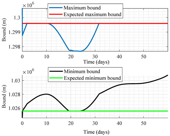
Figure 7. Relative motion-bound changing with time.

Due to the existence of atmospheric drag, the mean semi-major axis drops by 10 m every day without semi-major control, shown in Figure 8. It can be seen that the relative motion-bound control makes the semi-major axis of the deputy converge to that of the chief as well. That is because the expected bound values are fixed, and the fixed bounds exist only if the semi-major axis difference takes zero. Figure 9 shows the semi-major axes of the chief satellite and the deputy under semi-major axis control. The results indicate that the semi-major axes of the two satellites have been maintained around the expected value.

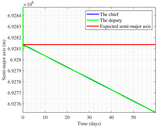
Figure 8. Semi-major axis time histories without semi-major axis control.

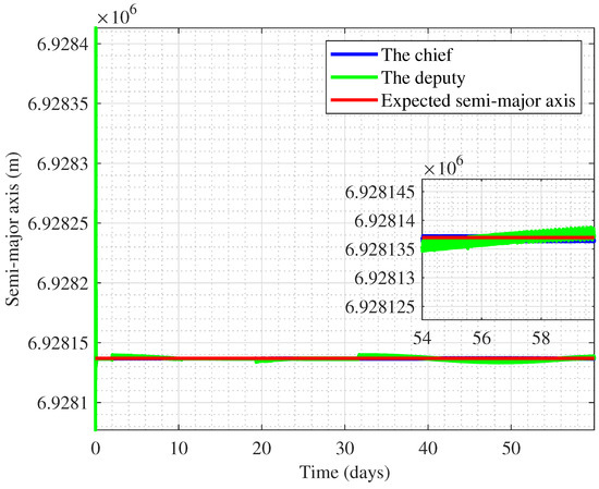
Figure 9. Semi-major axis time histories under semi-major axis control.

The control effect of the deputy is shown in Figure 10. The accumulated velocity increment is 1.98 m/s, and the single-step velocity increment is less than 0.02 m/s, which is minor enough for mega constellation control.

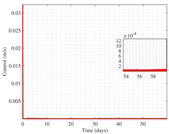
Figure 10. Control effects changing with time.

3.2. Self-Organizing Control of Coplanar Satellites

The coplanar satellites are selected as satellites of one orbit in GW-2 sub-constellation with an orbital altitude of 1145 km and inclination of ${60}^{\circ }$. The designed configuration of the GW-2 constellation has been presented in Table 1. There are 48 orbital planes and 36 coplanar satellites in the GW-2 sub-constellation total. The simulation parameters are listed in Table 3. The initial errors of $\delta \mathsf{\Omega },\delta \omega ,\delta f$ are relatively large, which simulate the drift of $\mathsf{\Omega },\omega ,f$ under perturbations without control.

Table 3. Simulation parameters for the coplanar satellites case.

Parameters	Values
Simulation Time	60 days
Step Length	600 s
Designed Configuration	$a_{\mathrm{t}}=R_{\mathrm{e}}+1145\mathrm{km}$
	$e_{\mathrm{t}}=0$
	$i_{\mathrm{t}}={60}^{\circ }$
	${\mathsf{\Omega }}_{\mathrm{t}}=0^{\circ }$
	${\omega }_{\mathrm{t}}=0^{\circ }$
Initial Orbit Errors	$\delta a=\left[-100,100\right]\mathrm{m},\mathrm{uniform}$
	$\delta e=\left[0,0.1\right],\mathrm{uniform}$
	$\delta i=\left[-0.1,0.1\right]deg,\mathrm{uniform}$
	$\delta \mathsf{\Omega }=\left[-10,10\right]deg,\mathrm{uniform}$
	$\delta \omega =\left[-1,1\right]deg,\mathrm{uniform}$
	$\delta f=\left[-1,1\right]deg,\mathrm{uniform}$
Perturbations	$J_2$, atmospheric drag, lunar gravity, solar gravity
Control Coefficients	$k_{\mathrm{bound}}=2\times {10}^{-8},k_a=2\times {10}^{-8}$
Ballistic Coefficient	$C_{D}A/\phantom{C_{D}Am}m=0.01$
Minimum Elevation Angle	$E_{min}={20}^{\circ }$

The angular radius of the coverage range is calculated as ${\alpha }_{max}={17.19}^{\circ }$. According to Equation (18), the RAAN drift should be within $\delta {\mathsf{\Omega }}_{min}=-{12.14}^{\circ }$ and $\delta {\mathsf{\Omega }}_{max}={12.14}^{\circ }$. The drift range of the relative motion bound can be calculated using Equations (15) and (20) based on the extreme value of $\delta \mathsf{\Omega }$.

The initial distribution of the coplanar satellites in the geocentric inertial system is shown in Figure 11, while the final distribution is shown in Figure 12. The red dots represent satellites that do not satisfy the continuous coverage constraint, named unqualified satellites, whereas the green dots represent satellites that satisfy the continuous coverage constraint. The number of unqualified satellites changing with time is shown in Figure 13. The unqualified satellites are reduced from 11 to 0 due to the self-organizing control, which verifies the feasibility of the proposed control method.

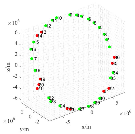
Figure 11. The initial distribution of the coplanar satellites in the geocentric inertial system. Red dots represent satellites that do not satisfy the continuous coverage constraint while green dots represent satellites that satisfy the continuous coverage constraint.

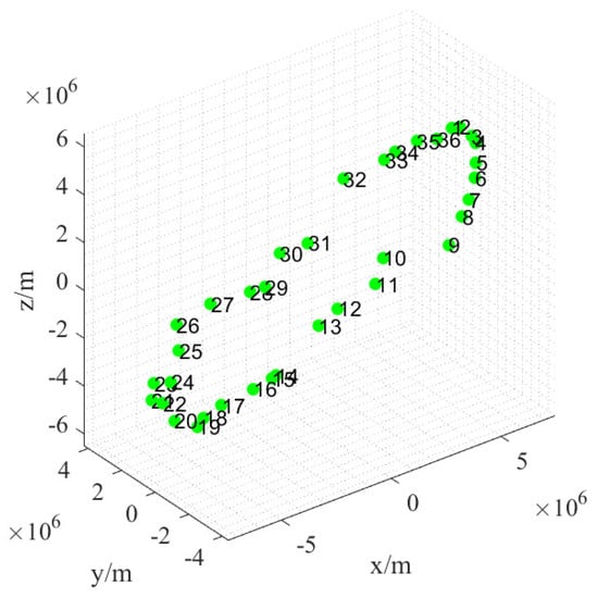
Figure 12. The final distribution of the coplanar satellites in the geocentric inertial system.

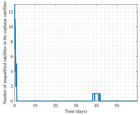
Figure 13. Number of unqualified satellites in the coplanar satellites.

The differences in the maximum relative motion bounds away from their corresponding constraints are shown in Figure 14. The differences should be negative theoretically and they actually are. Hence the maximum bound control has not been performed during the simulation time. The differences in the minimum relative motion bounds away from their corresponding constraints are shown in Figure 15, from which it can be found that all minimum bounds are controlled to be larger than the constraints. The occurrence of the unqualified satellite at 40 days in Figure 13 can be understood by referring to Figure 15. The small drift in the minimum bound away from the constraint due to perturbations is identified as unqualified.

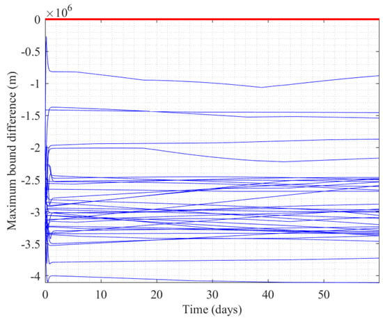
Figure 14. The differences in maximum bounds away from the corresponding constraints. Red line is zero-value standard. Blue lines are maximum bound differences.

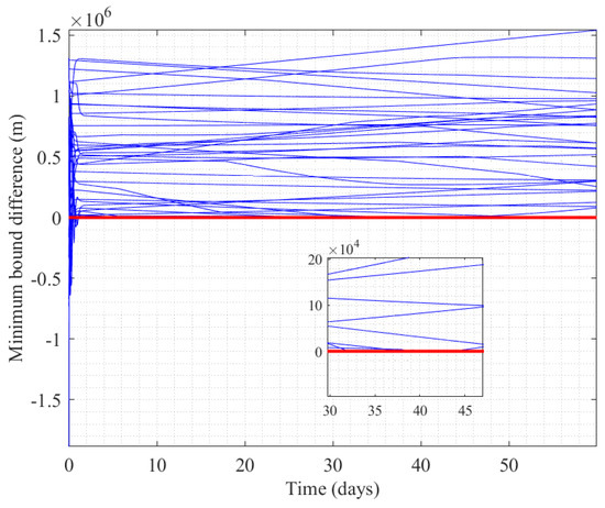
Figure 15. The differences in minimum bounds away from the corresponding constraints. Red line is zero-value standard. Blue lines are minimum bound differences.

The semi-major axis differences away from target value $a_{\mathrm{t}}$ are shown in Figure 16. The maximum drift of the semi-major axis at the final moment is 54.27 m. The RAAN differences away from the target RAAN under $J_2$ perturbation of the designed orbital plane are shown in Figure 17. The maximum drift of RAAN at the final moment is ${9.73}^{\circ }$. The control effects of coplanar satellites in the geocentric inertial system are shown in Figure 18. The exact velocity increments have no value of reference because the initial orbit conditions are dramatically bad. However, Figure 16 reveals the convergence of the proposed self-organizing control.

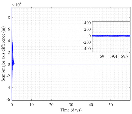
Figure 16. Semi-major axis differences away from the target value.

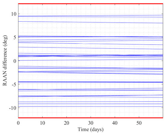
Figure 17. RAAN differences away from the target RAAN under $J_2$ perturbation. Red lines represent $\delta {\mathsf{\Omega }}_{\min }$ and $\delta {\mathsf{\Omega }}_{\max }$ respectively. Blue lines represent RAAN differences.

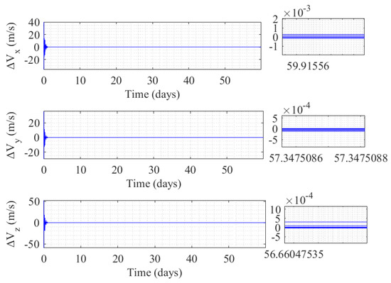
Figure 18. Control effects of coplanar satellites in the geocentric inertial system.

3.3. Self-Organizing Control of Mega Constellation

This paper focuses on self-organizing control to keep continuous coverage within the designed latitude zones, whereas collision avoidance control has not been considered so far. Since the proposed continuous coverage constraint relates to coplanar satellites only, the self-organizing control of different orbital planes is independent of each other.

The initial simulation parameters are listed in Table 4. In order to demonstrate the effect of relative motion-bound control, the initial errors of $\delta \mathsf{\Omega },\delta \omega ,\delta f$ are set as $\delta \mathsf{\Omega }\in \left[-5,5\right]deg$, $\delta \omega \in \left[-1,1\right]deg$, $\delta f\in \left[-1,1\right]deg$. The initial and final distributions of the mega constellation are shown in Figure 19 and Figure 20, respectively. Satellites that satisfy the continuous coverage constraint are colored green, while others are colored red. It can be observed that unqualified satellites turn into qualified satellites under self-organizing control. The number of unqualified satellites is reduced from 248 to 0, shown in Figure 21. The control effects in the geocentric inertial system changing with time are shown in Figure 22, which reveals the convergence of the proposed self-organizing control.

Table 4. Simulation parameters for the mega-constellation case.

Parameters	Values
Simulation Time	60 days
Step Length	600 s
Designed Configuration	$a_{\mathrm{t}}=R_{\mathrm{e}}+1145\mathrm{km}$
	$e_{\mathrm{t}}=0$
	$i_{\mathrm{t}}={60}^{\circ }$
	$P=48$
	$S=36$
Initial Orbit Errors	$\delta a=\left[-100,100\right]\mathrm{m},\mathrm{uniform}$
	$\delta e=\left[0,0.1\right],\mathrm{uniform}$
	$\delta i=\left[-0.1,0.1\right]deg,\mathrm{uniform}$
	$\delta \mathsf{\Omega }=\left[-5,5\right]deg,\mathrm{uniform}$
	$\delta \omega =\left[-1,1\right]deg,\mathrm{uniform}$
	$\delta f=\left[-1,1\right]deg,\mathrm{uniform}$
Perturbations	$J_2$, atmospheric drag, lunar gravity, solar gravity
Control Coefficients	$k_{\mathrm{bound}}=2\times {10}^{-8},k_a=2\times {10}^{-8}$
Ballistic Coefficient	$C_{D}A/\phantom{C_{D}Am}m=0.01$
Minimum Elevation Angle	$E_{min}={20}^{\circ }$

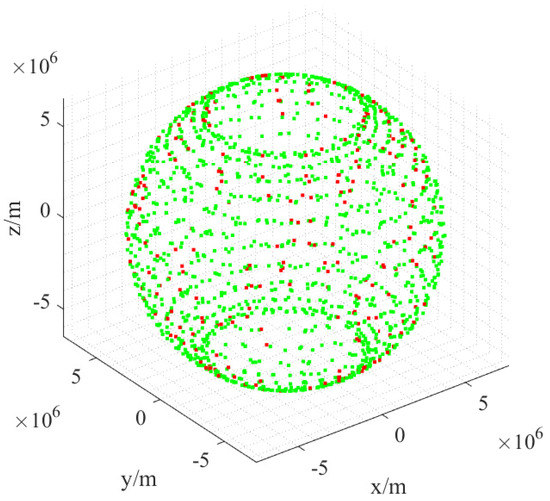
Figure 19. Initial distribution of the mega constellation. Red dots represent satellites that do not satisfy the continuous coverage constraint while green dots represent satellites that satisfy the continuous coverage constraint.

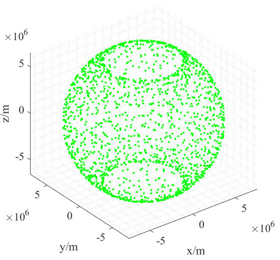
Figure 20. Final distribution of the mega constellation.

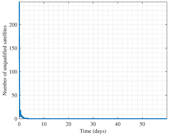
Figure 21. Number of unqualified satellites in the mega constellation.

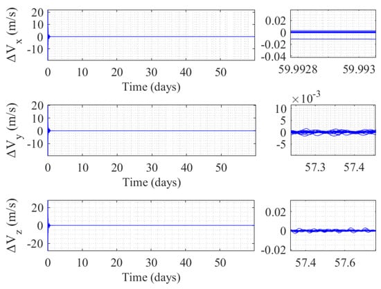
Figure 22. Control effects of constellation satellites.

The time histories of the maximum bound difference, minimum bound difference, semi-major axis difference, and RAAN difference are given in Figure 23, Figure 24, Figure 25 and Figure 26. All the minimum relative motion bounds converge to expected constraints automatically under control. The semi-major axis differences are restricted within 98.02 m, and the maximum drift of RAAN at the final moment is ${5.46}^{\circ }$, which is far away from the $\delta \mathsf{\Omega }$ drift constraint.

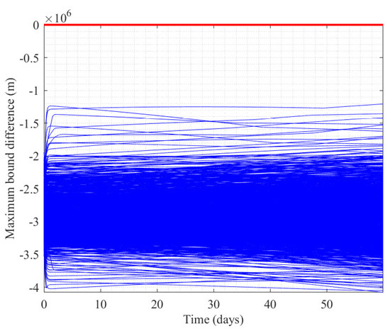
Figure 23. Maximum bound differences of constellation satellites. Red line is zero-value standard. Blue lines are maximum bound differences.

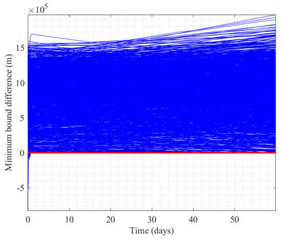
Figure 24. Minimum bound differences of constellation satellites. Red line is zero-value standard. Blue lines are minimum bound differences.

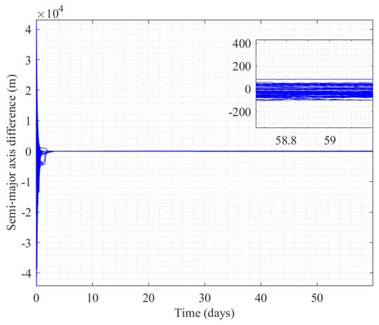
Figure 25. Semi-major axis differences of constellation satellites.

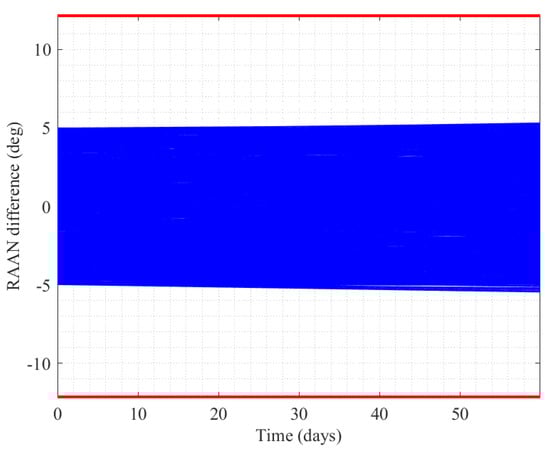
Figure 26. RAAN differences of constellation satellites. Red lines represent $\delta {\mathsf{\Omega }}_{\min }$ and $\delta {\mathsf{\Omega }}_{\max }$ respectively. Blue lines represent RAAN differences.

Figure 27 shows the coverage performance of the GW-2 sub-constellation at the final moment, where yellow dots represent virtual ground stations that can be single-covered, and red dots represent ground stations that cannot be single-covered. The results indicate that the GW-2 sub-constellation can provide continuous coverage within $\pm {78}^{\circ }$ along latitudes. Figure 28 shows the multiplicity of coverage of the GW-2 sub-constellation, where the blue curve denotes the initial condition and the green curve denotes the final condition. It can be found that the GW-2 constellation always provides continuous coverage within $\pm {78}^{\circ }$ latitude zones during the simulation time.

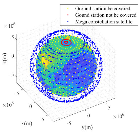
Figure 27. Coverage performance of the GW-2 sub-constellation.

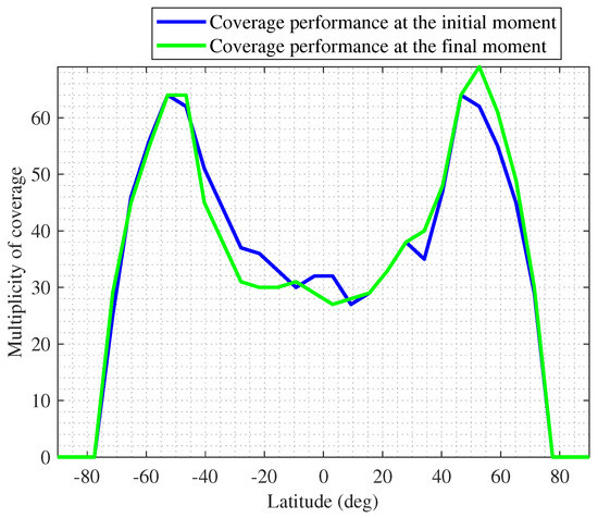
Figure 28. Multiplicity of coverage of the GW-2 sub-constellation at the initial and final moments.

4. Conclusions

In view of the numerous satellites in mega constellations, this paper innovatively introduces the self-organizing concept of mega constellation control. The emphasis is on realizing continuous Earth observation within the designed latitude zones so that the combination of multiple sub-constellations can provide global remote sensing services. A novel continuous coverage constraint has been presented that relates to intersatellite motion only, including the RAAN drift range and relative motion-bound drift range between two adjacent coplanar satellites. The configuration requirements for mega constellations have been studied, and most ongoing or planned mega constellations satisfy the proposed coverage constraint. Considering RAAN, the relative motion-bound and semi-major axis constraints, the corresponding artificial potential functions as well as the self-organizing rules have been designed. As a highlight, the scale-independent relative orbital elements are used as control variables in mega constellation control because these elements have high precision for near-circular orbits and arbitrary intersatellite ranges. The stability of satellite control using quadratic artificial potential functions has been proven. One key finding is that if the time derivative of the control variable is the same as that of the expected value under two-body Keplerian motion condition, the corresponding quadratic artificial potential function is stable. The self-organizing control simulations of coplanar satellites and the GW-2 sub-constellation have been carried out. The simulation results indicate the goodness of control effect for the small single-step velocity increment and low accumulated control consumption, and the mega constellation satisfies continuous coverage under control.

References

- Del Portillo, I.; Cameron, B.G.; Crawley, E.F. A technical comparison of three low earth orbit satellite constellation systems to provide global broadband. Acta Astronaut. 2019, 159, 123–135. [Google Scholar] [CrossRef]
- Williams, A.; Hainaut, O.; Otarola, A.; Tan, G.H.; Rotola, G. Analysing the impact of satellite constellations and ESO’s role in supporting the astronomy community. arXiv 2021, arXiv:2108.04005. [Google Scholar]
- Boggio, M.; Colangelo, L.; Virdis, M.; Pagone, M.; Novara, C. Earth Gravity In-Orbit Sensing: MPC Formation Control Based on a Novel Constellation Model. Remote Sens. 2022, 14, 2815. [Google Scholar] [CrossRef]
- Wang, Z.; Zhang, Y.; Wen, G.; Bai, S.; Cai, Y.; Huang, P.; Han, D.; He, Y. Atmospheric Density Model Optimization and Spacecraft Orbit Prediction Improvements Based on Q-Sat Orbit Data. arXiv 2021, arXiv:2112.03113. [Google Scholar]
- Mastro, P.; Masiello, G.; Serio, C.; Pepe, A. Change Detection Techniques with Synthetic Aperture Radar Images: Experiments with Random Forests and Sentinel-1 Observations. Remote Sens. 2022, 14, 3323. [Google Scholar] [CrossRef]
- Lang, T. Low Earth orbit satellite constellations for continuous coverage of the mid-latitudes. In Proceedings of the Astrodynamics Conference, San Diego, CA, USA, 29 July–31 July 1996; p. 3638. [Google Scholar]
- Santos, M.; Shapiro, B. Relating satellite coverage to orbital geometry. In Proceedings of the AIAA/AAS Astrodynamics Specialist Conference and Exhibit, Honolulu, HI, USA, 18–21 August 2008; p. 6609. [Google Scholar]
- Hackett, T.M.; Bilén, S.G.; Bell, D.J.; Lo, M.W. Geometric approach for analytical approximations of satellite coverage statistics. J. Spacecr. Rocket. 2019, 56, 1286–1299. [Google Scholar] [CrossRef]
- Dai, G.; Chen, X.; Wang, M.; Fernández, E.; Nguyen, T.N.; Reinelt, G. Analysis of satellite constellations for the continuous coverage of ground regions. J. Spacecr. Rocket. 2017, 54, 1294–1303. [Google Scholar] [CrossRef]
- Gong, Y.; Zhang, S.; Peng, X. Quick coverage analysis of mega Walker Constellation based on 2D map. Acta Astronaut. 2021, 188, 99–109. [Google Scholar] [CrossRef]
- Huang, S.; Colombo, C.; Bernelli-Zazzera, F. Multi-criteria design of continuous global coverage Walker and Street-of-Coverage constellations through property assessment. Acta Astronaut. 2021, 188, 151–170. [Google Scholar] [CrossRef]
- Arnas, D.; Casanova, D.; Tresaco, E. Relative and absolute station-keeping for two-dimensional–lattice flower constellations. J. Guid. Control. Dyn. 2016, 39, 2602–2604. [Google Scholar] [CrossRef]
- Chen, Y.; Zhao, L.; Liu, H.; Li, L.; Liu, J. Analysis of configuration and maintenance strategy of LEO walker constellation. J. Astronaut. 2019, 40, 1296–1303. [Google Scholar]
- Li, J.; Hu, M.; Wang, X.; Li, F.; Xu, J. Analysis of configuration offsetting maintenance method for LEO Walker constellation. Chin. Space Sci. Technol. 2021, 41, 38. [Google Scholar]
- Izzo, D.; Pettazzi, L. Autonomous and distributed motion planning for satellite swarm. J. Guid. Control. Dyn.s 2007, 30, 449–459. [Google Scholar] [CrossRef]
- Nag, S.; Summerer, L. Behaviour based, autonomous and distributed scatter manoeuvres for satellite swarms. Acta Astronaut. 2013, 82, 95–109. [Google Scholar] [CrossRef]
- Hu, Q.; Dong, H.; Zhang, Y.; Ma, G. Tracking control of spacecraft formation flying with collision avoidance. Aerosp. Sci. Technol. 2015, 42, 353–364. [Google Scholar] [CrossRef]
- McInnes, C.R. Autonomous proximity manoeuvring using artificial potential functions. ESA J. 1993, 17, 159–169. [Google Scholar]
- Cao, L.; Qiao, D.; Xu, J. Suboptimal artificial potential function sliding mode control for spacecraft rendezvous with obstacle avoidance. Acta Astronaut. 2018, 143, 133–146. [Google Scholar] [CrossRef]
- Spencer, D.A. Automated trajectory control using artificial potential functions to target relative orbits. J. Guid. Control. Dyn. 2016, 39, 2142–2148. [Google Scholar] [CrossRef]
- Wang, Z.; Xu, Y.; Jiang, C.; Zhang, Y. Self-organizing control for satellite clusters using artificial potential function in terms of relative orbital elements. Aerosp. Sci. Technol. 2019, 84, 799–811. [Google Scholar] [CrossRef]
- Xu, Y.; Wang, Z.; Zhang, Y. Bounded flight and collision avoidance control for satellite clusters using intersatellite flight bounds. Aerosp. Sci. Technol. 2019, 94, 105425. [Google Scholar] [CrossRef]
- Xu, Y.; Wang, Z.; Zhang, Y. Modeling and control of scale-independent relative orbital elements for near-circular orbits. Acta Astronaut. 2022, 198, 642–658. [Google Scholar]
- Jiang, C.; Wang, Z.; Zhang, Y. Decomposition analysis of spacecraft relative motion with different inter-satellite ranges. Acta Astronaut. 2019, 163, 56–68. [Google Scholar]
- An, M.; Wang, Z.; Zhang, Y. Self-organizing control strategy for asteroid intelligent detection swarm based on attraction and repulsion. Acta Astronaut. 2017, 130, 84–96. [Google Scholar] [CrossRef]
- Sun, Y.; Shen, H. The control of mega-constellation at low earth orbit based on TLE. Acta Astronaut. 2020, 42, 156. [Google Scholar]
Publisher’s Note: MDPI stays neutral with regard to jurisdictional claims in published maps and institutional affiliations. |
© 2022 by the authors. Licensee MDPI, Basel, Switzerland. This article is an open access article distributed under the terms and conditions of the Creative Commons Attribution (CC BY) license (https://creativecommons.org/licenses/by/4.0/).