A CNN Ensemble Based on a Spectral Feature Refining Module for Hyperspectral Image Classification

Abstract

In the study of hyperspectral image classification based on machine learning theory and techniques, the problems related to the high dimensionality of the images and the scarcity of training samples are widely discussed as two main issues that limit the performance of the data-driven classifiers. These two issues are closely interrelated, but are usually addressed separately. In our study, we try to kill two birds with one stone by constructing an ensemble of lightweight base models embedded with spectral feature refining modules. The spectral feature refining module is a technique based on the mechanism of channel attention. This technique can not only perform dimensionality reduction, but also provide diversity within the ensemble. The proposed ensemble can provide state-of-the-art performance when the training samples are quite limited. Specifically, using only a total of 200 samples from each of the four popular benchmark data sets (Indian Pines, Salinas, Pavia University and Kennedy Space Center), we achieved overall accuracies of 89.34%, 95.75%, 93.58%, and 98.14%, respectively.

1. Introduction

Hyperspectral image classification is a widely studied subject among remote sensing applications which are heavily dependent on machine learning theory and the related techniques [1]. The long lasting research interest for hyperspectral image classification is mainly due to the extremely high spectral resolution of hyperspectral images (HSIs), which is a very unique characteristic compared to natural images and other kinds of optical remote sensing images. HSIs with high spectral resolutions can be used to measure informative and distinctive spectral signatures of the ground surface. Therefore, HSIs are valuable to various applications, including resource management, environment monitoring and disaster analysis [2]. However, the high dimensionality of HSIs also makes HSI classification a challenging task. One critical issue is the Hughes phenomenon [3], which is caused by the high dimensionality of HSIs and the scarcity of training samples. In practical HSI classification tasks, the amount of labeled pixels which are available as training samples, is generally quite limited. These training samples result in being very sparse in the original high dimensional spectral feature space. Accordingly, they are often insufficient to support the training process of a complex machine learning model. Therefore, dimensionality reduction operations are usually included in HSI classification practices. Band selection is the most direct way to reduce the dimensionality of HSIs [4]. The flaw of band selection techniques is obviously that, in order to reduce information redundancy, some useful information will also be discarded by simply removing most of the spectral bands in HSIs. A more sophisticated choice is to adopt projection-based dimensionality reduction methods. Dimensionality reduction based on linear projection techniques, such as principle component analysis (PCA), independent component analysis (ICA) and factor analysis (FA), has typically been a standard preprocessing in HSI classification tasks for a long time [5]. On the other hand, nonlinear dimensionality reduction methods, such as those based on graphs and manifolds [6,7], are becoming more and more popular.

In recent years, there is an obvious growing trend that convolutional neural networks (CNNs) and other deep learning models are more and more popular in HSI classification tasks [8,9,10]. In order to make the CNN models more compatible with the unique characteristics of HSIs, many novel designs and exquisite structures have been proposed. As a pioneer work, the contextual deep CNN (CDCNN) [11] use a multi-scale convolutional filter bank to achieve a joint exploitation of the spatial and the spectral information in HSIs. In the diverse region-based CNN (DR-CNN) [12], six different shaped neighbor regions of a target pixel are extracted to provide richer spatial features for classifying the pixel. Besides extracting features from multiple scales and diverse regions, multi-model combination is also a widely adopted strategy in many HSI classification approaches. The two-stream model proposed in [13] uses a stacked denoising autoencoder to encode pixel-wise spectral values and a deep CNN to extract spatial features. In the spectral-spatial unified network (SSUN) [14], the pixel-wise analysis is implemented by a long short term memory (LSTM) module in parallel with a typical CNN established for patch-wise analysis and spatial feature extraction. In the double-branch multi-attention mechanism network (DBMA) [15], a CNN equipped with a channel attention module and another CNN equipped with a spatial attention module are combined to implement parallel spectral–spatial feature extraction. The usage of other attention modules has also been reported, such as the efficient channel attention (ECA) module embedded in the attention-based adaptive spectral–spatial kernel improved residual network (A2S2K-ResNet) proposed in [16]. There are also some very fresh works based on pure attention models, such as the model named spectralFormer proposed in [17]. As for single-stream models, such as the spectral–spatial residual network (SSRN) [18] and the hybrid spectral CNN (HybridSN) [19], 3D convolutions are usually adopted to achieve the simultaneous extraction of both the spectral and the spatial features in HSIs. In our previous work [20], we also used 3D convolutions together with dilated convolutions to achieve state-of-the-art performance on benchmark datasets. As compared to the basic 2D CNNs, 3D CNNs are usually more complex and require a larger amount of training samples.

In order to support the training processes of large CNN models using only a limited number of labeled samples, preprocessing steps, such as data augmentation and data generation, are usually implemented [21]. In [22], a ‘virtual sample enhanced’ method is presented to improve the training of the proposed 3D CNN by creating virtual training samples based on the mixture of real samples. In [23], data augmentation techniques based on image rotation and image flipping are adopted to increase the number of training samples up to six times. In [24], the idea of adversarial training is introduced into HSI classification tasks, and a multi-class spatial–spectral generative adversarial network (MSGAN), which contains two generator components and one discriminator component, is proposed. During the adversarial training procedure of MSGAN, one generator imitates the original training samples and generates synthetic samples containing only spectral information; the other one generates synthetic samples containing spatial information. These synthetic samples are given to the discriminator to improve its ability to classify real HSI samples.

Besides data augmentation and data generation, ensemble learning has also been verified as an effective technique to address the contradiction between large models and small training sets. The band-adaptive spectral–spatial feature learning neural network (Bass Net) proposed in [25] is an early stage deep neural network ensemble for HSI classification, which is based on an equal partition of the HSI spectral channels. A state-of-the-art performance on benchmark data sets was achieved by Bass Net without involving any kind of data augmentation. As compared to the idea of spectral feature partitioning used in Bass Net, random feature selection (RFS) is a more convenient and widely adopted manner to construct CNN ensembles for HSI classification [4]. As reported in [26], individual CNN classifiers with very simple structures are defined based on randomly selected spectral features extracted from the original HSIs. The resulting ensemble can produce highly accurate classifications after a training process based on the use of only a small amount of training samples. This work was improved later in [27] by introducing transfer learning [28] and employing pre-trained ImageNet models [29] as the base classifiers. The inspiration here is quite straightforward, i.e., the ensemble can be improved by enhancing the base classifiers. In [30], a model augmentation technique is proposed to synthesize new deep networks based on the original one by injecting Gaussian noise into the model’s weights, and this technique notably boosts the ensembles’ generalization ability over the unseen test data. In [31], the random oversampling of training samples is performed to enhance the training processes of base classifiers and therefore can improve the performance of the ensemble. Following a similar strategy, semi-supervised learning [32] and self-supervised learning [33] have also been introduced into the training processes of classification ensembles for HSIs.

In our study, we focus on the idea of using ensemble learning to solve the problems caused by the scarcity of training samples and the high dimensionality of HSIs. Instead of the RFS process, we propose a trainable spectral feature refining module as a very effective and convenient technique to construct ensembles of improved CNN classifiers. This spectral feature refining module consists of a channel attention computation and a 1 × 1 convolution layer, and it can be embedded into the CNN classifiers to support an end-to-end processing procedure. Unlike the independent RFS process, the spectral feature refining module can be trained along with the other layers within the base CNN classifier. Therefore, an optimized lower dimensional feature subspace can be produced by the module to support better classifications. The diversity among base classifiers in the ensemble is guaranteed by the inherent randomness of the training processes of the modules and the CNN models. The end-to-end fashion for training the base classifiers makes the proposed strategy more convenient than the RFS-based ensembles.

The main contributions of our study are twofold:

• We propose a trainable spectral feature refining module that is an effective dimensionality reduction technique for HSI classification. While the widely used projection-based dimensionality reduction techniques are usually implemented independently in the preprocessing stages of HSI classification tasks, the proposed spectral feature refining is more like an internal process of the classifier and can be optimized directly for improving the classification results.
• A new ensemble learning strategy for HSI classification is established based on the proposed spectral feature refining module and the inherent randomness of CNN models. Using such a simple strategy, it is quite convenient to produce diversity among base classifiers. Without explicitly splitting the original spectral feature space, the base classifiers are automatically trained on different low dimensional spectral feature subspaces produced by the embedded spectral feature refining modules.

The rest of this paper is organized as follows. As the two pillars of our proposal, the idea of ensemble learning and the mechanism of channel attention operations are discussed in Section 2. In Section 3, we describe the proposed ensemble model from its core mechanism to the overall architecture. Experimental comparisons between our proposal and the state-of-the-art approaches are reported in Section 4, followed by the conclusion of our study in Section 5.

2. Related Works

2.1. CNN Ensembles for HSI Classification

The main idea of ensemble learning is that, instead of using a large classifier, highly accurate and reliable classifications can also be obtained by establishing an ensemble of smaller classifiers. Since smaller classifiers are easier to train, the ensemble will be less demanding on the required amount of training samples. As stated in some classic works about ensemble learning [34], the error diversity among the predictions produced by the base classifiers is the key factor affecting the overall performance of an ensemble. If all the base classifiers make the same prediction, the ensemble cannot bring any improvements to the classification accuracy. Therefore, diverse individual predictions are pursued when an ensemble is established. According to the strategies adopted to create diversity, we divide the major existing CNN ensembles for HSI classification into four categories. We illustrate the differences between these strategies in Figure 1, where we take ensembles containing three base classifiers as examples.

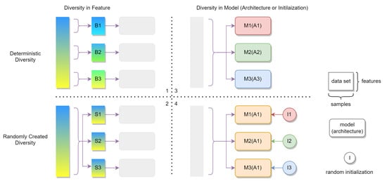
Figure 1. Four strategies (1, 2, 3, 4) for creating diversity within an ensemble of HSI classifiers. The rectangles represent different data sets, while the rounded rectangles represent the base classifiers. B1, B2 and B3 represent data sets corresponding to three contiguous sub-bands of the original HSI spectrum. S1, S2 and S3 represent data sets in three randomly selected spectral feature subspaces. A1, A2 and A3 are three different architectures for creating diversity in models, while I1, I2 and I3 represent three different initial states of the models created by the random initialization processes. Accordingly, an ensemble of three different models, denoted as M1, M2 and M3, can be created either with different architectures or with different initial states.

The aforementioned Bass Net [25] and TCNN ensemble [27] belong to the first two categories (labeled as 1 and 2 in Figure 1). Both ensembles use identical CNN models as base classifiers, and the diversity is obtained by constructing diverse training sets for different base classifiers. Since each new training set represents an unique subspace within the original feature space of HSIs, we denote this kind of diversity as feature-based diversity. The difference between these two categories relies on whether there is randomness in the feature subspace.

The other two categories (labeled as 3 and 4 in Figure 1) consist of ensembles directly established on different base models. We denote the corresponding strategy as model-based diversity. The aforementioned two-stream models, such as the one proposed in [13], can be considered simple ensembles following the strategy of category 3. In these ensembles, the two streams are the base models which are constructed with totally different deep network architectures. When the base models are CNNs, differences in architectures are not necessary for creating model-based diversity. The training processes of CNNs are based on random initialization and will converge to different states (especially) when the training samples are not abundant (the scarcity of training samples becomes an advantage here). It is therefore possible to train multiple CNNs with the same architecture using the same training set but still obtain different predictions for the same classification task. This very simple strategy was proved effective in models such as Hybra [35], which is an ensemble of multiple ResNets [36] and DenseNets [37].

Both the feature-based diversity and the model-based diversity have their own advantages. In ensembles using feature-based diversity, a dimensionality reduction procedure is implicitly included for each base classifier. Since the classifiers are established in some lower dimensional feature spaces, their structure can be smaller and their demands on training samples are also reduced. This is an implicit relief for the training sample scarcity problem. On the other hand, the advantage of the ensembles using model-based diversity is that no dedicated preprocessings are required.

It is not typical to see classic ensemble algorithms, such as bagging and boosting [38], being used in HSI classification tasks because these algorithms are based on a sub-sampling of the training samples, which obviously is not wise when the samples are already very scarce. Therefore, sampling-based ensembles are not included in our discussion.

2.2. Channel Attention

The attention mechanism is a much fresher technique compared to ensemble learning. It was introduced into vision-related research only a few years ago. However, because the attention mechanism is such an effective complement to the inefficiency of convolution operations to capture long range correlations, it has quickly become a preferred option for improving CNN models. There are two main types of attention mechanisms, which are known as spatial attention and channel attention. The attention mechanism has also been used in the study of HSI classification in recent years [39,40]. In some research, channel attention is also called spectral attention because different channels in a HSI represent different spectral features. However, the channel attention mechanism is usually not directly applied to the original spectral channels of HSIs, but is used to process intermediate stage feature maps in the data flow of CNN models.

The most classic channel attention mechanism is implemented in the squeeze-and-excitation (SE) block [41], which is illustrated in Figure 2. The SE block corresponds to an intermediate stage adaptive processing. The feature map $\mathbf{X}$, generated by the previous convolutional layer, is re-calibrated by the SE block to improve the feature extraction process of the following convolutional layers. The re-calibration of the feature map is achieved by assigning different weights to each channel in $\mathbf{X}$. These weights in the form of a vector are the output of a two-layer fully connected (FC) neural network, which takes the channel-wise global averages of $\mathbf{X}$ as inputs. Therefore, the channel attention vector is determined by $\mathbf{X}$ and the trainable parameters of the two-layer network. The effect of the feature re-calibration in the SE block is that the more important features in $\mathbf{X}$ are enhanced, whereas the less important ones are suppressed. The importance of the channels refers to whether they can contribute to the correct classifications of the model.

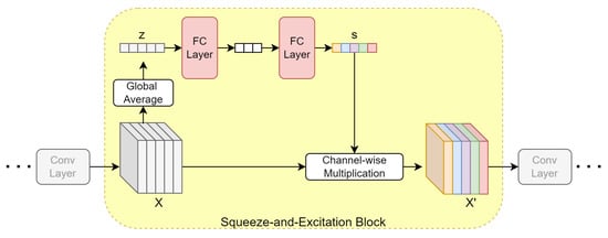
Figure 2. Implementation of the channel attention mechanism in a squeeze-and-excitation block.

The feature re-calibration process in an SE block can be described by the following equations:

$$\mathbf{z}\left(c\right)=\frac{1}{H\times W}\sum _{i=1}^H\sum _{j=1}^W\mathbf{X}\left(i,j,c\right)$$

(1)

$$\mathbf{s}=\sigma \left({\mathbf{W}}_2·\delta \left({\mathbf{W}}_1·\mathbf{z}\right)\right)$$

(2)

$${\mathbf{X}}^{\prime }\left(i,j,c\right)=\mathbf{s}\left(c\right)\times \mathbf{X}\left(i,j,c\right)$$

(3)

where $\mathbf{X},{\mathbf{X}}^{\prime }\in {\mathbb{R}}^{H\times W\times C}$ are the original feature map and the re-calibrated one; H, W, and C represent their heights, widths and channel numbers; and $\mathbf{z},\mathbf{s}\in {\mathbb{R}}^C$ are the channel descriptors and the scale vector, respectively. ${\mathbf{W}}_1\in {\mathbb{R}}^{C^{\prime }\times C}$ and ${\mathbf{W}}_2\in {\mathbb{R}}^{C\times C^{\prime }}$ are the weight matrices in the two-layer FC network; $\sigma$ and $\delta$ represent the nonlinear activation functions of sigmoid and ReLU [42].

In our study, we expand the usage of this channel attention mechanism from an intermediate stage processing to a preprocessing applied to the original HSIs. Moreover, we propose a spectral feature refining technique, which is based on this expansion of the channel attention mechanism.

3. Proposed Method

3.1. Channel Attention-Based Spectral Feature Refining

In our study, we use channel attention at the very front end of the model as a ‘soft’ spectral feature selection mechanism. The original spectral features corresponding to different HSI channels are weighted according to their impacts on the classification results. The channels assigned with large weights are considered the selected spectral features, whereas the unselected channels are suppressed by the small weights assigned to them. Since these suppressed feature channels cannot be discarded directly by this ‘soft’ feature selection mechanism, we use a small set of $1\times 1$ convolution kernels to reduce the dimensions of the weighted HSIs. As illustrated in Figure 3, we obtain a spectral feature refining (SFR) module, which can be embedded into almost any CNN model for HSI classification. Although the dimensionality of HSIs can be reduced by barely using the $1\times 1$ convolution layer, the channel attention operations in the module are still critical since they can improve the dimensionality reduction process. This is similar to the situations in which SE blocks are used to improve the feature extraction processes of convolution operations in many related research studies.

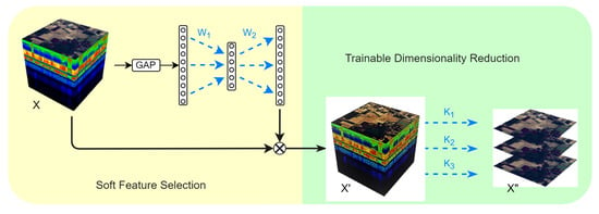
Figure 3. Data flow of the proposed spectral feature refining (SFR) module. GAP is short for global average pooling. ${\mathbf{W}}_1$ and ${\mathbf{W}}_2$ denote the parameters of the two fully connected layers. ${\mathbf{K}}_1$, ${\mathbf{K}}_2$ and ${\mathbf{K}}_3$ denotes three $1\times 1$ convolution kernels.

The ‘soft’ spectral feature selection process in the SFR module is mathematically the same as described in (1), (2) and (3), except that $\mathbf{X}$ represents the input HSI cube rather than an intermediate feature map. The dimensionality reduction process can be described as

$${\mathbf{X}}^{″}=\mathrm{CONCAT}\left({\mathbf{X}}^{\prime }\ast {\mathrm{K}}_1,{\mathbf{X}}^{\prime }\ast {\mathrm{K}}_2,{\mathbf{X}}^{\prime }\ast {\mathrm{K}}_3\right)$$

(4)

where $\mathrm{CONCAT}$ denotes the concatenation operation. ${\mathbf{X}}^{″}\in {\mathbb{R}}^{H\times W\times 3}$ is the output of the SFR module, which is a dimensionality reduced version of $\mathbf{X}$ with refined spectral channels.

Hereafter, we denote a CNN model equipped with the proposed SFR module as a spectral feature refining network (SFRN). An ordinary CNN model for HSI classification can be decomposed into two functional parts. The front part usually consists of several convolution layers with nonlinear activations and pooling operations. This part is in charge of semantic feature extraction. The rear part usually consists of some fully connected layers, including a softmax layer. This part is in charge of classification. The SFRN model proposed here contains three parts, namely the spectral feature refining part, the semantic feature extraction part and the classification part. Since the dimensionality of HSIs can be reduced by the spectral feature refining part, the dimensionality reduction operation for HSIs becomes an embedded component of the CNN model. The advantages of this embedded dimensionality reduction are as follows:

• It is more convenient since the process of dimensionality reduction is no longer an extra preprocessing step previous to the feature extraction and classification processes.
• Both the channel attention operation and the 1 × 1 convolution layer contain trainable parameters. Therefore, the spectral feature refining module can be optimized during the training stage of the SFRN model. This process not only reduces the dimensionality of HSIs, but also refines the spectral features for the classification task.
• More importantly, as in a SFRN, the training processes of the spectral feature refining part, the semantic feature extraction part and the classification part are implemented simultaneously using the same objective function. Hence, all the parts are optimized to the same direction.

3.2. SFRN Ensemble

We follow a patch-based manner to construct multiple SFRN models for our HSI classification tasks. During the training processes of the models, the trainable parameters are initialized randomly. Therefore, SFRN models with the same structure can be trained into different classifiers. Based on this inherent randomness in the training processes of our SFRN models, we construct an ensemble model which is denoted as SFRN ensemble hereafter.

The training process and the prediction process of the SFRN ensemble are illustrated in Figure 4. The structure of the individual SFRN classifier is quite simple. Besides the channel attention block, three 1 × 1 convolution kernels are included in the SFR module to reduce the dimensionality of the HSIs to three. The SFR module is followed by two convolution layers, both of which contain 64 convolution kernels with a ReLU activation function [43]. The rest part of the SFRN model consists of two fully connected layers containing 64 and M neurons respectively, where M represents the number of classes defined by the classification task. Multiple SFRN models are established as the base classifiers to construct our ensemble. The prediction of each base classifier will be a vector with M elements, which represents the possibilities that the input belongs to the M classes. All the base classifiers are trained independently using the same set of training samples, then their individual predictions for an unknown input are averaged to make the final classification. To be specific, the output vectors of the base classifiers are averaged as a single possibility vector. The decision is made by choosing the class with the largest possibility. As compared to CNN ensembles based on feature selection techniques, such as RFS, the proposed SFRN ensemble is much more convenient, as no preprocessing steps are required.

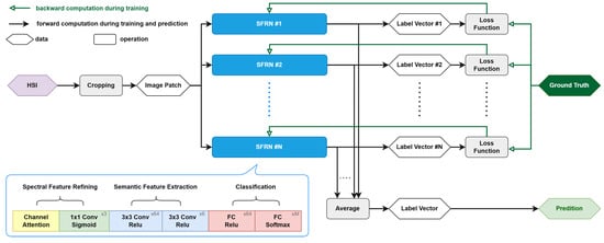
Figure 4. Data flow of the SFRN ensemble. Multiple identical base SFRN classifiers are trained in parallel, and the ensemble prediction for an unknown input is a simple average of the predictions produced by the base classifiers.

3.3. Discussion

As discussed in Section 2.1, different strategies for creating CNN ensembles have their own advantages. The feature-based ensemble is less demanding on the complexity and the power of the base model, while the model-based ensemble is preprocessing free. The ensemble proposed in this paper has both of these advantages at the same time since it follows a hybrid strategy by training randomly initialized CNN models in randomly created feature subspaces. Additionally, the whole ensemble is itself an end-to-end model, which can be conveniently implemented in practical applications. The hybrid strategy adopted in the proposed SFRN ensemble is illustrated in Figure 5.

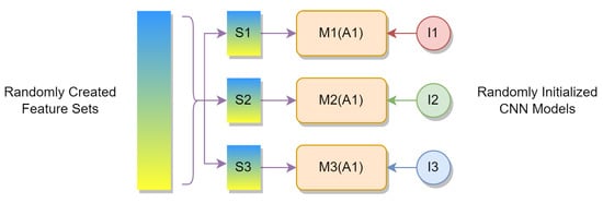
Figure 5. Hybrid strategy adopted in the proposed SFRN ensemble.

The main objective of the proposed approach is to take advantage of the rich spectral information provided by HSIs while alleviating the problems caused by the high dimensionality of HSIs. We also aim at promoting data-driven models for HSI classification when training samples are scarce. The SFRN ensemble is the comprehensive solution to meet all our research objectives. The spectral feature refining technique provides an optimized usage of the spectral features in HSIs, and the dimensionality reduction process is also implicitly included. Furthermore, both the ensemble framework and the dimensionality reduced feature space make it possible to obtain accurate classification results using only very simple CNN architectures with small amounts of labeled samples for training.

4. Experimental Results

4.1. Data Set Description and Experimental Setup

In our study, the performance of the proposed SFRN ensemble is evaluated on four classical HSI benchmark data sets, including the Indian Pines (IP) data set, the Salinas (SA) data set, the Pavia University (PU) data set and the Kennedy Space Center (KSC) data set [10]. Brief introductions about these data sets are as follows:

• The IP image was captured in 1992 by the 224-band airborne visible/infrared imaging spectrometer (AVIRIS) [44] over the Indian Pines test site in Northwestern Indiana, USA. The image contains $145\times 145$ pixels with a spatial resolution of 20 mpp. Here, 200 bands in the spectral range of 0.4–2.5 μm are selected out of the original image, then 10,249 pixels in the image are labeled and divided into 16 classes to form the data set.
• The SA data set is another data set gathered by the AVIRIS sensor. The campaign was conducted in 1998 over the agricultural area of Salinas Valley, California. The image contains $512\times 217$ pixels with a spatial resolution of 3.7 mpp. Here, 20 bands in the original image are discarded due to water absorption and noise. The data set contains 54,129 pixels belonging to 16 different classes.
• The PU image was captured by the reflective optics system imaging spectrometer (ROSIS) [45] over the campus of the University of Pavia, in the north of Italy. The image contains $610\times 340$ pixels with a spatial resolution of 1.3 mpp. After discarding the noisy bands, 103 out of the 115 original spectral bands, covering the spectral range from 0.43 to 0.86 μm, are kept to form the data set. It contains 42,776 pixels which can be categorized as nine different classes that belong to an urban environment with multiple solid structures, natural objects and shadows.
• The KSC image was also captured by the AVIRIS sensor. The campaign was conducted in 1996 over the neighborhood of the Kennedy Space Center in Florida, USA. The image contains $512\times 614$ pixels with a spatial resolution of 18 mpp. Only 176 spectral bands ranging from 0.4 to 2.5 μm are kept in the data set, which contains 5211 labeled pixels belonging to 13 different land cover classes.

Four sets of comparative experiments were conducted. The first experiment is a comparison between the SFR module and the PCA-based dimensionality reduction. This is to study the saturation phenomenon in the band selection process for HSI classification, and it is also to demonstrate the superiority of the SFR module as an optimized dimensionality reduction technique. In the second experiment, the SFRN ensemble is compared with some state-of-the-art (SOTA) HSI classification models. This experiment is to verify that the proposed ensemble is capable of improving the performance of very simple CNN models to the level of those of SOTA CNN models with very complex structures. In the third experiment, the SFRN ensemble is compared with other ensembles for HSI classification. This is to verify the effectiveness of the proposed convenient strategy to construct reliable ensembles which can make accurate predictions based on small amounts of training samples. Ablation analysis is also performed by comparing ensembles of SFRNs, CDRNs and basic CNNs. This is the fourth set of experiments conducted in our study. The overall accuracy (OA), the average accuracy (AA) and the kappa coefficient are the metrics involved in our experiments to evaluate the classification results of different models.

The experiments are conducted on an Intel Xeon E5 platform equipped with 64 GB memory and a Nvidia Geforce GTX 1080Ti graphic processing unit. The proposed SFRN ensemble is implemented based on the framework of Tensorflow. The source code is available on Github (https://github.com/modestyao/SFRN-ensemble, accessed on 7 October 2022). More details about the programming environment can be found on our source code page. In the first two sets of experiments, all the results are obtained in our own programs, while in the third experiment, the accuracy metrics of the existing ensembles are cited from the original paper. This is because we have no access to the source codes of these ensemble approaches and therefore cannot reproduce their experiments fairly.

4.2. Spectral Redundancy and Dimensionality Reduction

The purpose of the first experiment is to evaluate the SFR module as an effective dimensionality reduction technique for HSI classification. Four different dimensionality reduction processes, including the one based on the SFR module, are implemented and compared with each other in the experiment. The PCA-based approach is the most classic one which has been widely used and is still quite popular in recent researches. The FA-based approach is also very effective for reducing a large number of variables into fewer numbers of factors. The convolution-based dimensionality reduction (CDR) can be considered the prototype of the SFR module. As discussed in Section 3.1, the dimensionality of HSIs can be reduced by barely using a $1\times 1$ convolution layer, and the channel attention operation in the SFR module can further improve the spectral features with reduced dimensions.

A very simple CNN model with only two convolution layers is employed as the objective model working on the spectral feature subspaces created by different dimensionality reduction approaches. The structure of this objective model is illustrated in Figure 6. The objective model is trained using 10% of the labeled samples in each of the four benchmark data sets, and the overall accuracies of its predictions are estimated on the remaining samples. Patches corresponding to the $9\times 9$ neighborhood of the samples are cropped from the images after the dimensionality reduction operations. These patches are constructed as the inputs to the classification model. The number of epochs for training the model is set to 50. We use the Adam optimizer for the training processes, and the learning rate is set to 0.001. We repeat the experiments for five times and the means and standard deviations (STDs) of the OA values are illustrated in Figure 7. We denote the classification results achieved by the model on different spectral subspaces created by the four dimensionality reduction approaches as PCA, FA, CDR and SFR, respectively.

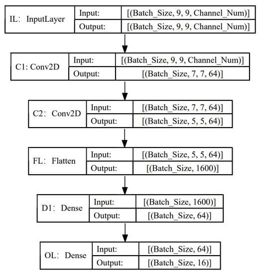
Figure 6. Structure of the objective CNN model. The major parts of this network include two convolutional layers and two fully connected layers. Two sets of 64 $3\times 3$ convolution filters are used in the two convolutional layers.

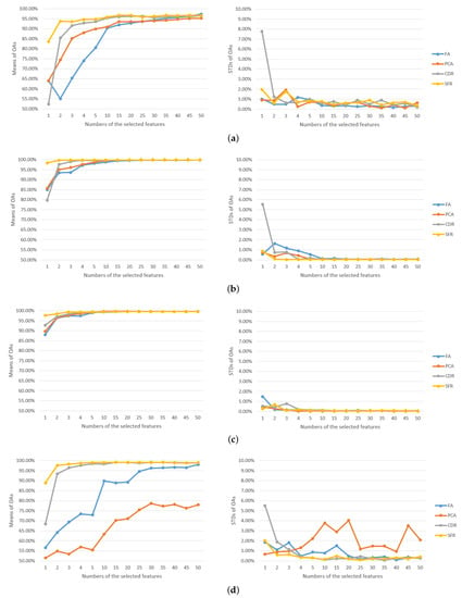
Figure 7. Classification results obtained by the objective CNN model on different spectral feature subspaces created by four dimensionality reduction approaches, respectively. The model is trained using 10% of the samples in each of the four data sets. (a) IP, (b) SA, (c) PU, (d) KSC.

Since we are using a quite small model, most of the accuracy curves show a trend to saturate rapidly when the dimensions of the inputs increase. Both the PCA-based dimensionality reduction process and the FA-based dimensionality reduction process are implemented based on the internal structures of the data sets, while CDR and SFR are optimized for the classification tasks. Therefore, it is not surprising to see that the CNN model produces less accurate classification results on the feature spaces created by the the two projection-based approaches, especially when the dimensionality of the feature space is lower than five. When the dimensionality is higher than 10, the accuracies corresponding to the four different dimensionality reduction approaches are very close to each other on the data sets of SA and PU. On the IP data set, the advantages of the proposed SFR dimensionality reduction approach over the projection-based ones are more obvious, while the accuracy curves are also quite similar to each other when the dimensionality is higher than 30. The situation is quite different on the KSC data set. The PCA dimensionality reduction approach leads to very poor classification results even when the dimensionality is only reduced to 50. The FA curve looks better, but the accuracies are also quite low when the dimensionality is lower than 10. On the contrary, SFR and CDR lead to much better classification results. In particular, the accuracies corresponding to SFR are constantly higher than 95% when the dimensionality is higher than two. The reason for the poor performances of the PCA and the FA approaches is that the labeled samples only take a very small percentage among the pixels in the whole image. The projection-based approaches are optimized for the whole image, while CDR and SFR are optimized only for the labeled samples. CDR and SFR are more “task-oriented” and hence can support better classifications. In general, for any of the four data sets, the SFR module can help the CNN model to produce accurate classifications even when the spectral dimensionality of the data set is largely reduced. The improvements from CDR to SFR are also very obvious on all the data sets involved in our experiments.

4.3. Classification Performance

The second part of our experimental analysis is related to the comparisons between the proposed SFRN ensemble and the SOTA HSI classification approaches. In these comparisons, the implementation of the SFRN ensemble (SFRN-E) consists of 10 SFRNs as the base classifiers, and the structures of these SFRNs in the ensemble are exactly the same as illustrated in Figure 4, except for that they take 11 × 11 patches as inputs. SFRN-E is compared with five SOTA models, namely CDCNN [11], SSRN [18], DBMA [15], HybridSN [19] and SpectralNet [46]. In each of the 10 base SFRN classifier in our ensemble, we use the SFR module to reduce the dimensionality of the original HSIs to three. The randomness of the SFR-based dimensionality reduction process will guarantee the diversity of the obtained three-dimensional feature spaces. This means that we can obtain 30 different feature dimensions in the ensemble. For the other single-model approaches, we reduce the dimensionality of the HSIs to 30 before constructing our training samples. Therefore, both our ensemble and the SOTA models are trained on 30-dimensional feature spaces. This gives our comparative experiment a certain level of fairness. All the models are trained using a total of 200 samples in each of the four benchmark data sets. These samples are randomly selected from all the categories according to their proportions within each data set. The performance of the models is estimated on the remaining samples, as reported in Table 1, Table 2, Table 3 and Table 4. The amounts of samples in the training set and the test set are also reported. The per-class classification accuracies are measured using the F1-score; OA, AA and the kappa coefficients are reported to demonstrate the overall performance of different models.

Table 1. Classification accuracies on the test set obtained by different approaches on the IP dataset (200 samples are used for training and the rest for test). Best results are pointed out in bold.

Label	Class Name	Training/Test	CDCNN	SSRN	DBMA	HybridSN	SpectralNet	SFRN-E
1	Alfalfa	2/44	42.72	46.15	68.24	88.61	56.82	82.67
2	Corn-notill	25/1403	58.82	71.83	73.58	66.92	65.72	89.06
3	Corn-mintill	13/817	46.15	77.43	70.44	56.60	69.25	65.19
4	Corn	3/234	29.59	25.19	52.70	38.62	25.74	64.76
5	Grass-pasture	7/476	89.15	80.87	80.92	75.83	64.39	84.67
6	Grass-trees	12/718	94.25	94.15	88.68	93.99	81.46	87.88
7	Grass-pasture-mowed	1/27	9.76	0.00	25.00	66.67	46.67	75.00
8	Hay-windrowed	14/464	94.14	97.71	96.30	75.51	99.46	97.83
9	Oats	1/19	12.24	0.00	0.00	58.18	25.00	27.50
10	Soybean-notill	25/947	68.74	78.04	80.29	75.19	74.90	87.67
11	Soybean-mintill	48/2407	75.75	85.08	86.76	86.00	79.05	94.62
12	Soybean-clean	11/582	44.89	52.61	71.08	53.75	60.06	75.74
13	Wheat	4/201	82.06	86.44	85.09	81.82	96.68	96.16
14	Woods	28/1237	92.49	91.36	94.77	96.14	90.81	97.37
15	Buildings-Grass-Trees-Drives	5/381	66.67	24.35	53.99	54.77	51.50	52.69
16	Stone-Steel-Towers	1/92	70.27	55.93	17.82	42.11	35.77	62.94
OA(%)			72.03 ± 1.29	78.48 ± 0.96	80.86 ± 1.80	77.07 ± 2.51	75.07 ± 2.03	86.39 ± 0.92
AA(%)			62.88 ± 1.71	57.42 ± 2.98	64.70 ± 2.74	70.30 ± 3.66	61.07 ± 3.24	75.87 ± 2.60
Kappa × 100			68.03 ± 1.49	75.30 ± 1.12	78.10 ± 2.06	73.83 ± 2.84	71.05 ± 2.31	84.44 ± 1.03

Table 2. Classification accuracies on the test set obtained by different approaches on the SA dataset (200 samples are used for training and the rest for test). Best results are pointed out in bold.

Label	Class Name	Training/Test	CDCNN	SSRN	DBMA	HybridSN	SpectralNet	SFRN-E
1	Brocoli_green_weeds_1	7/2002	99.98	100.00	98.84	99.63	76.06	98.50
2	Brocoli_green_weeds_2	14/3712	96.80	99.93	99.92	99.72	85.63	99.68
3	Fallow	7/1969	99.46	95.57	96.63	91.48	91.97	98.41
4	Fallow_rough_plow	5/1389	92.84	98.55	96.58	95.59	95.96	93.63
5	Fallow_smooth	10/2668	95.20	98.39	95.83	96.49	97.16	96.36
6	Stubble	15/3944	99.23	100.00	99.23	96.34	99.51	99.39
7	Celery	13/3566	99.92	99.87	99.86	99.87	94.49	98.87
8	Grapes_untrained	42/11,229	83.50	88.04	92.06	94.06	82.08	92.81
9	Soil_vinyard_develop	23/6180	99.19	99.72	99.57	100.00	98.66	99.51
10	Corn_senesced_green_ weeds	12/3266	92.70	94.12	93.56	98.00	92.27	95.92
11	Lettuce_romaine_4wk	4/1064	93.53	96.61	92.26	79.50	74.97	97.38
12	Lettuce_romaine_5wk	7/1920	96.75	99.12	99.46	100.00	91.57	95.29
13	Lettuce_romaine_6wk	3/913	83.38	98.85	99.51	91.91	93.38	92.92
14	Lettuce_romaine_7wk	4/1066	90.86	96.44	94.42	82.45	97.20	94.42
15	Vinyard_untrained	27/7241	76.69	78.13	90.00	92.05	76.31	89.89
16	Vinyard_vertical_trellis	7/1800	98.24	99.20	98.28	80.57	92.08	99.02
OA(%)			91.40 ± 0.48	93.82 ± 0.51	95.70 ± 0.37	95.15 ± 0.92	88.42 ± 1.47	95.75 ± 0.27
AA(%)			94.09 ± 0.75	96.41 ± 0.90	97.31 ± 0.39	93.69 ± 1.63	89.98 ± 1.35	96.59 ± 0.44
Kappa × 100			90.44 ± 0.54	93.11 ± 0.58	95.22 ± 0.42	94.61 ± 1.02	87.13 ± 1.64	95.27 ± 0.29

Table 3. Classification accuracies on the test set obtained by different approaches on the PU dataset (200 samples are used for training and the rest for test). Best results are pointed out in bold.

Label	Class Name	Training/ Test	CDCNN	SSRN	DBMA	HybridSN	SpectralNet	SFRN-E
1	Asphalt	31/6600	88.86	91.80	95.28	85.37	85.94	91.39
2	Meadows	87/18,562	96.53	97.53	97.10	97.69	92.32	98.70
3	Gravel	10/2089	64.82	75.81	76.92	76.90	59.11	79.62
4	Trees	14/3050	92.51	94.04	94.35	68.37	89.11	93.70
5	Painted metal sheets	6/1339	99.96	99.87	99.32	88.40	95.64	99.51
6	Bare Soil	24/5005	86.51	91.63	90.16	92.83	79.42	94.93
7	Bitumen	6/1324	74.95	91.74	91.95	78.20	66.00	88.84
8	Self-Blocking Bricks	17/3665	75.49	84.00	81.86	71.76	82.03	78.30
9	Shadows	5/942	78.65	91.37	94.42	53.26	70.27	90.47
OA(%)			89.70 ± 0.76	93.25 ± 0.89	93.33 ± 0.77	88.25 ± 3.42	86.36 ± 2.04	93.58 ± 0.89
AA(%)			83.77 ± 1.90	90.35 ± 1.37	91.44 ± 1.28	79.16 ± 7.83	77.15 ± 2.28	89.01 ± 1.26
Kappa × 100			86.27 ± 0.98	91.05 ± 1.16	91.17 ± 1.02	84.31 ± 4.68	81.51 ± 2.56	91.46 ± 1.18

Table 4. Classification accuracies on the test set obtained by different approaches on the KSC dataset (200 samples are used for training and the rest for test). Best results are pointed out in bold.

Label	Class Name	Training/Test	CDCNN	SSRN	DBMA	HybridSN	SpectralNet	SFRN-E
1	Scrub	29/732	85.20	88.54	84.00	96.85	89.27	100.00
2	Willow swamp	9/234	78.74	77.29	68.78	79.53	67.02	91.03
3	CP hammock	10/246	86.56	93.14	84.94	93.75	59.66	97.07
4	Slash pine	10/242	64.79	80.72	71.36	78.44	42.86	90.42
5	Oak/Broadleaf	6/155	61.86	75.86	65.55	76.87	73.97	88.26
6	Hardwood	9/220	61.21	74.01	66.81	89.50	69.72	100.00
7	Swamp	4/101	64.76	65.22	80.46	79.56	87.83	88.40
8	Gramionoi marsh	17/414	95.48	93.51	77.83	97.62	65.59	97.30
9	Spartina marsh	20/500	90.96	93.30	86.12	96.59	80.47	99.70
10	Cattail marsh	15/389	89.45	91.50	84.38	99.62	75.28	100.00
11	Salt marsh	16/403	75.19	79.20	72.29	86.97	91.18	100.00
12	Mud flats	19/484	89.16	88.66	80.82	94.55	77.79	100.00
13	Water	36/891	95.91	95.02	96.74	96.01	96.42	100.00
OA(%)			85.05 ± 0.99	88.15 ± 1.40	82.18 ± 2.00	92.96 ± 1.43	79.82 ± 2.01	98.14 ± 0.18
AA(%)			80.18 ± 0.92	81.67 ± 2.25	76.95 ± 2.44	88.49 ± 1.59	74.92 ± 2.53	95.54 ± 0.47
Kappa × 100			83.36 ± 01.09	86.73 ± 1.61	80.10 ± 2.23	92.14 ± 1.62	77.53 ± 2.25	97.93 ± 0.20

SFRN-E outperforms all the compared approaches on the four data sets, in terms of overall accuracy. As regarding to class-wise accuracies, SFRN-E produced the best classification results on seven out of the 16 classes in the IP dataset, and this proportion is 12/13 for the dataset of KSC. All the class-wise accuracies achieved by SFRN-E are above 90%, on 15 out of the 16 classes in the SA dataset. This is a noticeably more stable and balanced performance as compared to the other models. On the PU dataset, SFRN-E also achieved the best class-wise results on three out of the nine classes. A very important advantage of SFRN-E is the consistency of its performance across different datasets. As a contrast, the performance of DBMA is quite close to SFRN-E on the datasets of SA and PU, but it drops a lot on the dataset of KSC. In general, the advantage of SFRN-E is more obvious on the IP and the KSC data sets, which contain fewer labeled samples as compared to the other two data sets. This can be considered as verification of the ability of SFRN to deal with the scarcity of training samples.

Visual comparisons are also included here, as illustrated in Figure 8, Figure 9, Figure 10 and Figure 11. Classification maps produced by different approaches are compared with the ground truths. In general, the classification maps produced by the SFRN ensemble show fewer mislabeled areas as compared to the maps produced by the other approaches.

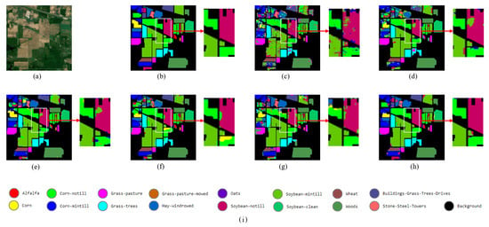
Figure 8. Visual assessments of the classification maps produced by different approaches on the IP data set. Some local details are highlighted to demonstrate the differences in the classification results. (a) False color image; (b) Ground truth; (c) CDCNN; (d) SSRN; (e) DBMA; (f) HybridSN; (g) SpectralNet; (h) SFRN-E; (i) Legends.

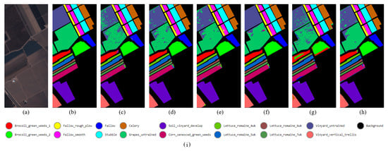
Figure 9. Visual assessments of the classification maps produced by different approaches on the SA data set. (a) False color image; (b) Ground truth; (c) CDCNN; (d) SSRN; (e) DBMA; (f) HybridSN; (g) SpectralNet; (h) SFRN-E; (i) Legends.

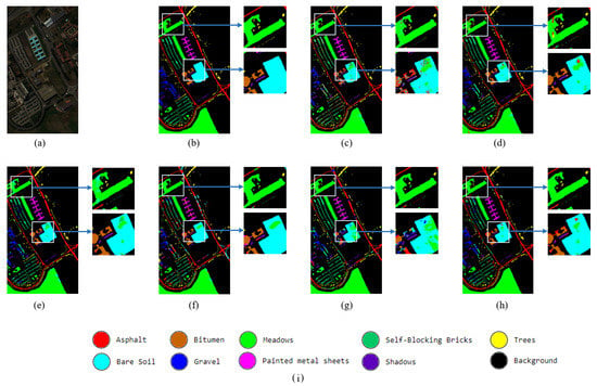
Figure 10. Visual assessments of the classification maps produced by different approaches on the PU data set. Some local details are highlighted to demonstrate the differences in the classification results. (a) False color image; (b) Ground truth; (c) CDCNN; (d) SSRN; (e) DBMA; (f) HybridSN; (g) SpectralNet; (h) SFRN-E; (i) Legends.

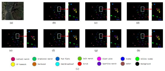
Figure 11. Visual assessments of the classification maps produced by different approaches on the KSC data set. Some local details are highlighted to demonstrate the differences in the classification results. (a) False color image; (b) Ground truth; (c) CDCNN; (d) SSRN; (e) DBMA; (f) HybridSN; (g) SpectralNet; (h) SFRN-E; (i) Legends.

4.4. Comparisons with Other Ensembles

The third experiment is to compare the proposed SFRN ensemble with other ensembles. The comparisons are partially based on the experimental results reported in [27]. As discussed in Section 1, ensemble learning is introduced into the tasks of HSI classification as an alternative to data augmentation techniques when the amount of labeled samples is not large enough to fully support the training of a complex CNN model. In our experiment, we select only 200 samples from each data set to train the SFRN ensemble and then we evaluate the ensemble using the remaining samples. As in the second experiment, we use 10 SFRNs as the base classifiers to construct our ensemble. The Adam optimizer is adopted, and the learning rate is uniformly set to 0.001 for the training processes of all the base classifiers. The numbers of training epochs are set to 50. For the sake of fair comparisons, we follow the settings in [27] by repeating the training and evaluation processes of our ensemble 10 times, and the averages and standard deviations of accuracies achieved on the test sets are recorded and compared with the recordings reported in [27]. As shown in Table 5, four ensembles are considered for comparisons, including an ensemble of support vector machine (SVM-E), a CNN ensemble (CNN-E), a CNN ensemble with transfer learning (TCNN-E) and a CNN ensemble with transfer learning and improved label smoothing (TCNN-E-ILS). As in Section 4.3, SFRN-E in Table 5 represents the implementation of the proposed SFRN ensemble. Inspired by the label smoothing process applied in [27], we also include label smoothing into the training processes of our base SFRN classifiers.

Table 5. Classification results produced by different ensembles, using only 200 samples in each data set for training and the rest for test. Best results are pointed out in bold. The accuracies are the averages obtained in 10 repeated experiments, and the stand deviations are also reported.

Data Sets	Metrics	SVM-E	CNN-E	TCNN-E	TCNN-E	SFRN-E
					(with Label Smoothing)	(with Label Smoothing)
	OA(%)	81.61 ± 1.47	88.62 ± 0.36	90.17 ± 2.16	91.88 ± 1.13	91.62 ± 0.45
IP	AA(%)	57.51 ± 4.24	66.55 ± 3.49	71.53 ± 5.83	77.37 ± 4.04	80.02 ± 0.91
	Kappa × 100	77.62 ± 1.83	86.30 ± 0.43	88.21 ± 2.60	90.28 ± 1.34	90.43 ± 0.51
	OA(%)	-	84.02	87.94	89.62	94.18 ± 0.35
PU	AA(%)	-	83.71	82.98	85.14	89.34 ± 0.58
	Kappa × 100	-	84.76	84.21	86.51	92.25 ± 0.47
	OA(%)	91.57 ± 2.47	96.85 ± 0.69	97.29 ± 1.51	99.27 ± 0.36	99.28 ± 0.30
KSC	AA(%)	87.10 ± 3.43	95.90 ± 0.94	96.06 ± 2.14	98.87 ± 0.64	98.33 ± 0.67
	Kappa × 100	90.60 ± 2.76	96.50 ± 0.76	96.98 ± 1.68	99.19 ± 0.41	99.20 ± 0.33

These ensembles are evaluated on three data sets, namely IP, PU and KSC. Since the SA data set is not included in the experiments reported in [27], we cannot compare the performance of SFRN-E with the other ensembles on this data set. The overall classification performances are reported in Table 5, in terms of OAs, AAs and kappa coefficients. SVM-E, CNN-E and TCNN-E are all established on the randomness of the random feature selection process. This preprocessing is abandoned in SFRN-E by converting it into an internal module of the base CNN classifier. SFRN outperforms SVM-E and CNN-E on all the three datasets. The overall performance results of SFRN-E and TCNN-E are close to each other on the data sets of IP and KSC, but SFRN-E is much more reliable on the data set of PU. Considering the fact that TCNN-E is an ensemble of pretrained CNNs, SFRN-E is much easier to construct. The experimental results confirm the effectiveness of this more convenient strategy adopted in our study to construct CNN ensembles.

Another interesting phenomenon that can be observed in the experimental results is that the performance of the ensemble is largely correlated with the base classifiers. Since the ability of CNN models to extract spatial features from images is much stronger than that of SVMs, all the CNN ensembles outperform SVM-E. Furthermore, the ensemble of CNN can be improved when the individual CNN models are enhanced. This kind of improvement can be achieved by adopting techniques, such as transfer learning and label smoothing, as shown by the comparison between CNN-E, TCNN-E and TCNN-E trained with label smoothing. The SFR module proposed in our study can also be considered as a very effective technique to improve the individual CNN models in the ensemble. On the IP and KSC data sets, the performance improvements brought by the SFR module are roughly equivalent to transfer learning, while on the PU data set, the SFR is obviously a much more effective boosting technique. Meanwhile, when the SFR module is used together with label smoothing, the performance of the ensemble will be further improved.

The total numbers of the parameters in different models, including the proposed SFRN ensemble, TCNN-E, HybridSN and the others involved in our study, are reported in Table 6. The size of the proposed SFRN ensemble is much smaller than TCNN-E, and it is even smaller than HybridSN. This indicates the advantage of the proposed ensemble as a low complexity model which can provide comparable or even better classification results as compared to those very complex models. It should be pointed out that these parameter numbers only correspond to the models established for the KSC dataset. For the other datasets with different class numbers, the sizes of these models will also be different, but the order of size will remain consistent.

Table 6. Total number of parameters in different models established for the KSC data set.

Models	CDCNN	SSRN	DBMA	HybridSN	SpectralNet	CNN-E	TCNN-E	SFRN-E
Parameter Amount	0.303 M	0.310 M	0.06 M	6.781 M	6.802 M	1.118 M	34.822 M	2.721 M

4.5. Ablation Analysis

The ablation study is conducted by modifying and removing the SFR modules from the SFRNs in the proposed ensemble. Specifically, four ensembles composed of different types of base classifiers are constructed and compared with each other. There are 10 base classifiers in each of these ensembles, and the differences between the structures of their base classifiers are illustrated in Figure 12. In the figure, “CNN” denotes the very simple CNN structure as explained in Section 4.2. When we replace the SFR module in SFRN with a CDR module, we obtain the CDR network (CDRN) as our base classifier. The proposed SFR module is based on the SE block, and in the original study, SE blocks are used in the middle part of CNNs. Therefore, we remove the SFR module from the top of SFRN and insert it between the two convolutional layers in the network. We denote this variant of the base classifier in our ensemble as “SENet”. The SFRN ensemble and its variants are compared on the data sets of IP, SA, PU and KSC. A total of 200 samples out of each dataset are selected for training the base classifiers in different ensembles. We still use the Adam optimizer and the learning rate is still 0.001 during all the training processes. Each training process still consists of 50 epochs.

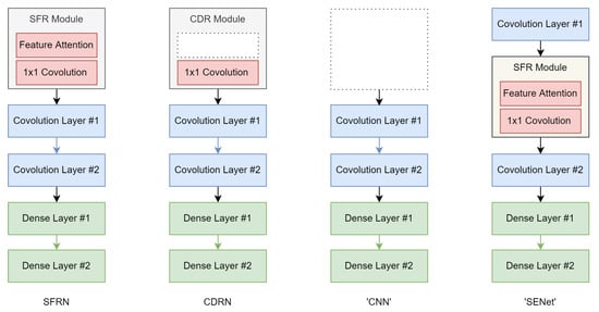
Figure 12. Different types of base classifiers to construct the ensemble.

As reported in Table 7, the improvements from the “CNN” ensemble to the CDRN ensemble and then to the SFRN ensemble are quite obvious. A performance increase of at least five percent in terms of OA can be observed when comparing the “CNN” ensemble with the SFRN ensemble. This demonstrates the effectiveness of the SFR module as a task-oriented dimensionality reduction technique. The comparison between the CDRN ensemble and the SFRN ensemble reveals the necessity to include the spectral attention based soft feature selection operation in our dimensionality reduction approach. The results produced by the “SENet” ensemble are comparable to the SFRN ensemble, but the overall advantages of SFRN ensemble are still notable.

Table 7. Ablation analysis. Best results are pointed out in bold. The accuracies are the averages obtained in 10 repeated experiments, and the stand deviations are also reported.

Data Sets	Metrics	“CNN” Ensemble	CDRN Ensemble	“SENet” Ensemble	SFRN Ensemble
	OA(%)	73.31 ± 0.25	88.33 ± 0.94	90.75 ± 0.24	91.62 ± 0.45
IP	AA(%)	65.00 ± 0.35	72.74 ± 2.61	78.41 ± 0.65	80.02 ± 0.91
	Kappa × 100	69.34 ± 0.28	86.60 ± 1.09	89.83 ± 0.28	90.43 ± 0.51
	OA(%)	90.26 ± 0.15	94.47 ± 0.33	95.06 ± 0.09	95.46 ± 0.18
SA	AA(%)	92.65 ± 0.18	95.83 ± 0.56	97.35 ± 0.23	97.02 ± 0.42
	Kappa × 100	89.15 ± 0.17	93.84 ± 0.37	94.50 ± 0.10	94.95 ± 0.19
	OA(%)	89.77 ± 0.14	90.46 ± 0.38	92.78 ± 0.37	94.18 ± 0.35
PU	AA(%)	86.89 ± 0.22	83.65 ± 0.93	88.55 ± 0.99	89.34 ± 0.58
	Kappa × 100	86.30 ± 0.19	87.23 ± 0.52	90.35 ± 0.51	92.25 ± 0.47
	OA(%)	59.07 ± 0.47	97.31 ± 0.35	99.06 ± 0.14	99.28 ± 0.30
KSC	AA(%)	46.54 ± 0.91	93.65 ± 0.76	97.32 ± 0.42	98.33 ± 0.67
	Kappa × 100	54.20 ± 0.55	97.00 ± 0.39	98.96 ± 0.16	99.20 ± 0.33

5. Conclusions

This paper presents ensemble learning for HSI classification as an alternative solution to the training sample scarcity problem. As a common phenomenon in machine learning researches, the training processes of simpler models are less demanding on the amounts of required training samples, while ensemble learning is an effective technique to promote the performance of simple models. Therefore, when the training samples are not sufficient to support the training process of a complex CNN model, ensembles of simpler models can be exploited. Following such an idea, we propose a quite convenient approach to construct a very effective CNN ensemble for HSI classification, based on a novel spectral feature refining module and the inherent randomness in the initialization of CNNs.

Besides the proposed approach for HSI classification, a very important theoretical contribution in our study is the combination between a solution to the training sample scarcity problem and a solution to the problems caused by the high dimensionality of HSIs. An implicit dimensionality reduction is included in the spectral feature refining module, which is the base for the ensemble. Experimental results demonstrate that the proposed ensemble is a reliable choice for HSI classification tasks when training samples are scarce, and the proposed module is also an effective technique for dimensionality reduction.

As the base classifier in the proposed ensemble, SFRN is a model featured by its very simple structure. However, the SFRN ensemble as a whole is still a rather big model. As compared to single-model approaches, the training process for any type of classification ensemble can be more time consuming, especially when the ensemble contains a large amount of base classifiers. We suppose that this is probably the main reason why ensemble learning is less popular for small dataset problems, such as HSI classification. Therefore, improving the efficiency of the classification model will be the main goal in our future study. In fact, we have already started to research knowledge distillation techniques for HSI classification tasks.

References

- Camps-Valls, G.; Tuia, D.; Bruzzone, L.; Benediktsson, J.A. Advances in Hyperspectral Image Classification: Earth Monitoring with Statistical Learning Methods. IEEE Signal Process. Mag. 2014, 31, 45–54. [Google Scholar] [CrossRef]
- Tong, Q.; Xue, Y.; Zhang, L. Progress in Hyperspectral Remote Sensing Science and Technology in China Over the Past Three Decades. IEEE J. Sel. Top. Appl. Earth Obs. Remote Sens. 2014, 7, 70–91. [Google Scholar] [CrossRef]
- Hughes, G. On the mean accuracy of statistical pattern recognizers. IEEE Trans. Inf. Theory 1968, 14, 55–63. [Google Scholar] [CrossRef]
- Xia, J.; Liao, W.; Chanussot, J.; Du, P.; Song, G.; Philips, W. Improving random forest with ensemble of features and semisupervised feature extraction. IEEE Geosci. Remote Sens. Lett. 2015, 12, 1471–1475. [Google Scholar] [CrossRef]
- Falco, N.; Benediktsson, J.A.; Bruzzone, L. Spectral and spatial classification of hyperspectral images based on ICA and reduced morphological attribute profiles. IEEE Trans. Geosci. Remote Sens. 2015, 53, 6223–6240. [Google Scholar] [CrossRef]
- Shi, G.; Huang, H.; Liu, J.; Li, Z.; Wang, L. Spatial-spectral multiple manifold discriminant analysis for dimensionality reduction of hyperspectral imagery. Remote Sens. 2019, 11, 2414. [Google Scholar] [CrossRef]
- Shah, C.; Du, Q. Spatial-Aware Collaboration-Competition Preserving Graph Embedding for Hyperspectral Image Classification. IEEE Geosci. Remote Sens. Lett. 2022, 19, 1–5. [Google Scholar] [CrossRef]
- Paoletti, M.E.; Haut, J.M.; Plaza, J.; Plaza, A. Deep learning classifiers for hyperspectral imaging: A review. ISPRS J. Photogramm. Remote Sens. 2019, 158, 279–317. [Google Scholar] [CrossRef]
- Li, S.; Song, W.; Fang, L.; Chen, Y.; Ghamisi, P.; Benediktsson, J.A. Deep learning for hyperspectral image classification: An overview. IEEE Trans. Geosci. Remote Sens. 2019, 57, 1–20. [Google Scholar] [CrossRef]
- Audebert, N.; Le Saux, B.; Lefèvre, S. Deep learning for classification of hyperspectral data: A comparative review. IEEE Geosci. Remote Sens. Mag. 2019, 17, 159–173. [Google Scholar] [CrossRef]
- Lee, H.; Kwon, H. Going deeper with contextual CNN for hyperspectral image classification. IEEE Trans. Image Process. 2017, 26, 4843–4855. [Google Scholar] [CrossRef] [PubMed]
- Zhang, M.; Li, W.; Du, Q. Diverse region-based CNN for hyperspectral image classification. IEEE Trans. Image Process. 2018, 27, 2623–2634. [Google Scholar] [CrossRef] [PubMed]
- Hao, S.; Wang, W.; Ye, Y.; Nie, T.; Bruzzone, L. Two-stream deep architecture for hyperspectral image classification. IEEE Trans. Geosci. Remote Sens. 2018, 56, 2349–2361. [Google Scholar] [CrossRef]
- Xu, Y.; Zhang, L.; Du, B.; Zhang, F. Spectral-spatial unified networks for hyperspectral image classification. IEEE Trans. Geosci. Remote Sens. 2018, 56, 5893–5909. [Google Scholar] [CrossRef]
- Ma, W.; Yang, Q.; Wu, Y.; Zhao, W.; Zhang, X. Double-branch multi-attention mechanism network for hyperspectral image classification. Remote Sens. 2019, 11, 1307. [Google Scholar] [CrossRef]
- Roy, S.K.; Manna, S.; Song, T.; Bruzzone, L. Attention-based adaptive spectral-spatial kernel ResNet for hyperspectral image classification. IEEE Trans. Geosci. Remote Sens. 2020, 59, 1–13. [Google Scholar] [CrossRef]
- Hong, D.; Han, Z.; Yao, J.; Gao, L.; Zhang, B.; Plaza, A.; Chanussot, J. SpectralFormer: Rethinking Hyperspectral Image Classification with Transformers. IEEE Trans. Geosci. Remote Sens. 2022, 60, 1–5. [Google Scholar] [CrossRef]
- Zhong, Z.; Li, J.; Luo, Z.; Chapman, M. Spectral-spatial residual network for hyperspectral image classification: A 3D deep learning framework. IEEE Trans. Geosci. Remote Sens. 2018, 56, 847–858. [Google Scholar] [CrossRef]
- Roy, S.K.; Krishna, G.; Dubey, S.R.; Chaudhuri, B.B. HybridSN: Exploring 3D-2D CNN feature hierarchy for hyperspectral image classification. IEEE Geosci. Remote Sens. Lett. 2019, 17, 1–5. [Google Scholar] [CrossRef]
- Xu, H.; Yao, W.; Cheng, L.; Li, B. Multiple spectral resolution 3D convolutional neural network for hyperspectral image classification. Remote Sens. 2021, 13, 1248. [Google Scholar] [CrossRef]
- Chang, Y.L.; Tan, T.H.; Lee, W.H.; Chang, L.; Chen, Y.N.; Fan, K.C.; Alkhaleefah, M. Consolidated Convolutional Neural Network for Hyperspectral Image Classification. Remote Sens. 2022, 14, 1571. [Google Scholar] [CrossRef]
- Chen, Y.; Jiang, H.; Li, C.; Jia, X.; Ghamisi, P. Deep feature extraction and classification of hyperspectral images based on convolutional neural networks. IEEE Trans. Geosci. Remote Sens. 2016, 54, 6232–6251. [Google Scholar] [CrossRef]
- Zhang, Y.; Huynh, C.P.; Ngan, K.N. Feature fusion with predictive weighting for spectral image classification and segmentation. IEEE Trans. Geosci. Remote Sens. 2019, 57, 1–16. [Google Scholar] [CrossRef]
- Feng, J.; Yu, H.; Wang, L.; Cao, X.; Zhang, X.; Jiao, L. Classification of hyperspectral images based on multiclass spatial-spectral generative adversarial networks. IEEE Trans. Geosci. Remote Sens. 2019, 57, 5329–5343. [Google Scholar] [CrossRef]
- Santara, A.; Mani, K.; Hatwar, P.; Singh, A.; Garg, A.; Padia, K.; Mitra, P. Bass net: Band-adaptive spectral-spatial feature learning neural network for hyperspectral image classification. IEEE Trans. Geosci. Remote Sens. 2017, 55, 5293–5301. [Google Scholar] [CrossRef]
- Chen, Y.; Wang, Y.; Gu, Y.; He, X.; Ghamisi, P.; Jia, X. Deep learning ensemble for hyperspectral image classification. IEEE J. Sel. Top. Appl. Earth Obs. Remote Sens. 2019, 12, 1882–1897. [Google Scholar] [CrossRef]
- He, X.; Chen, Y. Transferring CNN ensemble for hyperspectral image classification. IEEE Geosci. Remote Sens. Lett. 2021, 18, 1–5. [Google Scholar] [CrossRef]
- Pan, S.J.; Yang, Q. A Survey on Transfer Learning. IEEE Trans. Knowl. Data Eng. 2010, 22, 1345–1359. [Google Scholar] [CrossRef]
- Russakovsky, O.; Deng, J.; Su, H.; Krause, J.; Satheesh, S.; Ma, S.; Huang, Z.; Karpathy, A.; Khosla, A.; Bernstein, M.; et al. ImageNet Large Scale Visual Recognition Challenge. Int. J. Comput. Vis. 2015, 115, 211–252. [Google Scholar] [CrossRef]
- Nalepa, J.; Myller, M.; Tulczyjew, L.; Kawulok, M. Deep Ensembles for Hyperspectral Image Data Classification and Unmixing. Remote Sens. 2021, 13, 4133. [Google Scholar] [CrossRef]
- Lv, Q.; Feng, W.; Quan, Y.; Dauphin, G.; Gao, L.; Xing, M. Enhanced-Random-Feature-Subspace-Based Ensemble CNN for the Imbalanced Hyperspectral Image Classification. IEEE J. Sel. Top. Appl. Earth Obs. Remote Sens. 2021, 14, 3988–3999. [Google Scholar] [CrossRef]
- Manian, V.; Alfaro-Mejía, E.; Tokars, R.P. Hyperspectral Image Labeling and Classification Using an Ensemble Semi-Supervised Machine Learning Approach. Sensors 2022, 22, 1623. [Google Scholar] [CrossRef] [PubMed]
- Liu, B.; Gao, K.; Yu, A.; Ding, L.; Qiu, C.; Li, J. ES2FL: Ensemble Self-Supervised Feature Learning for Small Sample Classification of Hyperspectral Images. Remote Sens. 2022, 14, 4236. [Google Scholar] [CrossRef]
- Brown, G.; Wyatt, J.; Harris, R.; Yao, X. Diversity creation methods: A survey and categorisation. Inf. Fusion 2005, 6, 5–20. [Google Scholar] [CrossRef]
- Minetto, R.; Segundo, M.P.; Sarkar, S. Hydra: An ensemble of convolutional neural networks for geospatial land classification. IEEE Trans. Geosci. Remote Sens. 2019, 57, 1–12. [Google Scholar] [CrossRef]
- He, K.; Zhang, X.; Ren, S.; Sun, J. Deep Residual Learning for Image Recognition. In Proceedings of the IEEE Conference on Computer Vision and Pattern Recognition (CVPR), Las Vegas, NV, USA, 27–30 June 2016. [Google Scholar]
- Huang, G.; Liu, Z.; van der Maaten, L.; Weinberger, K.Q. Densely connected convolutional networks. In Proceedings of the IEEE/CVF Conference on Computer Vision and Pattern Recognition (CVPR), Honolulu, HI, USA, 21–26 July 2017; pp. 4700–4708. [Google Scholar]
- Zhou, Z.; Wu, J.; Tang, W. Ensembling neural networks: Many could be better than all. Artif. Intell. 2002, 137, 239–263. [Google Scholar] [CrossRef]
- Mei, X.; Pan, E.; Ma, Y.; Dai, X.; Huang, J.; Fan, F.; Du, Q.; Zheng, H.; Ma, J. Spectral-spatial attention networks for hyperspectral image classification. Remote Sens. 2019, 11, 963. [Google Scholar] [CrossRef]
- Sun, H.; Zheng, X.; Lu, X.; Wu, S. Spectral-spatial attention network for hyperspectral image classification. IEEE Trans. Geosci. Remote Sens. 2020, 58, 3232–3245. [Google Scholar] [CrossRef]
- Hu, J.; Shen, L.; Sun, G. Squeeze and excitation networks. In Proceedings of the IEEE/CVF Conference on Computer Vision and Pattern Recognition (CVPR), Salt Lake City, UT, USA, 18–23 June 2018. [Google Scholar]
- Nair, V.; Hinton, G.E. Rectified linear units improve restricted boltzmann machines. In Proceedings of the International Conference on Machine Learning (ICML), Haifa, Israel, 21–24 June 2010; pp. 807–814. [Google Scholar] [CrossRef]
- Glorot, X.; Bordes, A.; Bengio, Y. Deep sparse rectifier neural networks. In Proceedings of the 14th International Conference on Artificial Intelligence and Statistics (AISTATS), Fort Lauderdale, FL, USA, 11–13 April 2011; pp. 315–323. [Google Scholar]
- Green, R.O.; Eastwood, M.L.; Sarture, C.M.; Chrien, T.G.; Aronsson, M.; Chippendale, B.J.; Faust, J.A.; Pavri, B.E.; Chovit, C.J.; Solis, M.; et al. Imaging Spectroscopy and the Airborne Visible/Infrared Imaging Spectrometer (AVIRIS). Remote Sens. Environ. 1998, 65, 227–248. [Google Scholar] [CrossRef]
- Kunkel, B.; Blechinger, F.; Lutz, R.; Doerffer, R.; van der Piepen, H.; Schroder, M. ROSIS (Reflective Optics System Imaging Spectrometer)—A candidate instrument for polar platform missions. In Proceedings of the Optoelectronic Technologies for Remote Sensing from Space, Cannes, France, 17–20 November 1987; Bowyer, C.S., Seeley, J.S., Eds.; International Society for Optics and Photonics, SPIE: Bellingham, WA, USA, 1988; Volume 0868, pp. 134–141. [Google Scholar] [CrossRef]
- Chakraborty, T.; Trehan, U. SpectralNET: Exploring Spatial-Spectral WaveletCNN for Hyperspectral Image Classification. arXiv 2021, arXiv:2104.00341. [Google Scholar]
Publisher’s Note: MDPI stays neutral with regard to jurisdictional claims in published maps and institutional affiliations. |
© 2022 by the authors. Licensee MDPI, Basel, Switzerland. This article is an open access article distributed under the terms and conditions of the Creative Commons Attribution (CC BY) license (https://creativecommons.org/licenses/by/4.0/).