Article

Multiscale Normalization Attention Network for Water Body Extraction from Remote Sensing Imagery

1
College of Computer and Information, Hohai University, Nanjing 211100, China
2
Key Laboratory of Water Big Data Technology of Ministry of Water Resources, Hohai University, Nanjing 211100, China
3
Tongshan Water Conservancy Bureau, Xuzhou 221116, China
*
Authors to whom correspondence should be addressed.
Remote Sens. 2022, 14(19), 4983; https://doi.org/10.3390/rs14194983
Submission received: 25 August 2022 / Revised: 28 September 2022 / Accepted: 4 October 2022 / Published: 7 October 2022
(This article belongs to the Special Issue Computer Vision and Machine Learning Application on Earth Observation)

Abstract

:
Extracting water bodies is an important task in remote sensing imagery (RSI) interpretation. Deep convolution neural networks (DCNNs) show great potential in feature learning; they are widely used in the water body interpretation of RSI. However, the accuracy of DCNNs is still unsatisfactory due to differences in the many hetero-features of water bodies, such as spectrum, geometry, and spatial size. To address the problem mentioned above, this paper proposes a multiscale normalization attention network (MSNANet) which can accurately extract water bodies in complicated scenarios. First of all, a multiscale normalization attention (MSNA) module was designed to merge multiscale water body features and highlight feature representation. Then, an optimized atrous spatial pyramid pooling (OASPP) module was developed to refine the representation by leveraging context information, which improves segmentation performance. Furthermore, a head module (FEH) for feature enhancing was devised to realize high-level feature enhancement and reduce training time. The extensive experiments were carried out on two benchmarks: the Surface Water dataset and the Qinghai–Tibet Plateau Lake dataset. The results indicate that the proposed model outperforms current mainstream models on OA (overall accuracy), f1-score, kappa, and MIoU (mean intersection over union). Moreover, the effectiveness of the proposed modules was proven to be favorable through ablation study.

1. Introduction

Water plays an important role in human social and economic development [1]. Accurate mapping of water bodies is of great significance for environment monitoring and water resource management. Satellite remote sensing is widely used in surface water body interpretation because of its low labor cost and speed [2]. Water has complicated spectrum features due to its diversity in salinity, dust, microorganisms, and shadow effects, which brings challenges to water body extraction from remote sensing imagery (RSI) [3]. In addition, the extraction accuracy is limited because of huge variances of water-body in geometry and spatial size. The purpose of this study is to realize high-accuracy water-body extraction from RSI.
Traditional methods manually extract water bodies from multispectral RSI with water features such as normalized difference water index (NDWI) [4] and modified normalized difference water index (MNDWI) [5]. They perform well when the dataset is low in noise, but it is inaccessible in real scenes and lacks certain generalization ability. For timely water body extraction, the traditional methods still have some shortcomings, such as a low level of automation and manual dependence. Consequently, the traditional water body extraction methods have deficiencies under the current massive remote sensing data conditions.
Convolutional neural networks (CNNs) are tremendous superior in learning feature representation and pattern recognition. Fully convolutional networks (FCNs) were firstly proposed in 2015, representing a pioneering type of semantic segmentation network [6]. Fully connected layer is replaced by convolution layer in FCN, which realizes feature mapping from image pixels to semantic categories. Nevertheless, continuous pooling operation discards too much detailed information, resulting in deficiencies in semantic segmentation accuracy. Attempting to address the aforementioned problems, many optimized versions have been proposed. Ronneberger et al. reused encoder features by using skip connection during upsampling in U-Net, which is widely used in medical image interpretation [7]. Badrinarayanan et al. proposed a more structured model named SegNet, which uses the maximum pooling index to fuse more information in the encoder, boosting the boundary classification accuracy [8]. Zhao et al. proposed the pyramid scene parsing network (PSPNet), which integrates the context information based on different regions with the pyramid pooling module [9]. Chen et al. proposed the DeeplabV3+ model, which uses dilated convolution to expand the receptive field, and adopts the atrous spatial pyramid pooling (ASPP) module to capture multiscale semantic information [10]. Schlemper et al. introduced the attention mechanism (AM) into U-Net, which has been proven to be effective in improving the classification ability of the model [11].
As an important research branch of computer vision, AM is widely used in RSI semantic segmentation [12]. It realizes spatial or channel information enhancement by injecting weight vectors into the learned features, which improves model performance and does not introduce multiple parameters at a time. More specifically, AM can avoid the omission of much key detailed information, which is regarded as a vital factor affecting the performance.
RSI implies inherent complex spectral and spatial information. Simultaneously, the semantic features that are abstracted from these properties contribute to correctly classifying water bodies from sufficient clues. Therefore, Miao et al. proposed a novel edge loss function, which effectively mitigates the boundary blur problem [13]. Similarly, He et al. utilized edge information guidance in pursuit of improving the performance [14]. Wang et al. designed a shape feature optimization module to optimize the shape structure of water bodies, which improves their structural similarity [15]. The core of these strategies is to enhance the accuracy of water extraction by leveraging boundary information, but this kind of method always performs conservatively in case significant differences exist in the water spectrum. In order to address this problem, Weng et al. expanded the receptive field through dilated convolution to enhance feature representation [16]. Guo et al. proposed a multiscale feature extractor to ensure the accuracy of water body extraction [17]. Zhang et al. proposed a multiscale encoder network to improve the semantic segmentation accuracy of RSI [18]. Li et al. proposed a cross-level context network to augment the distinguishability of features, enabling the model to make more accurate judgments [19]. Wang et al. proposed a network based on multiscale attention and transfer learning which obtained satisfactory results [20]. Zhang et al. devised a multiscale feature extraction module to realize semantic feature fusion and achieve high-accuracy extraction of water bodies from satellite and aerial imagery [21]. For methods based on channel attention mechanisms, channels that are more informative are chosen to train the model. This is helpful for enhancing the classification ability of the model. However, it compresses the whole channel-wise feature into a single value, resulting in the loss of some key information. Consequently, some tiny water bodies cannot be identified in real applications.
Firstly, it is very important to make full use of multiscale information to enhance the representation of water features [22,23,24]. In addition, speeding up the training of the model while ensuring accuracy has great value for the practicality of the model [25]. We suppose that these are the main reasons that hinder the practicability and accuracy of the model. Accordingly, a multiscale normalization attention network (MSNANet) is proposed in this study. In general, the main contributions are as follows:
  • To enhance the attention representation of water body semantic features, a multiscale normalization attention (MSNA) module was designed. It utilizes BN to obtain weights rather than global average pooling (GAP), which reduces the amount of parameters in the model and retains spatial information concurrently. In addition, a grouping strategy used in MSNA augments feature representations with multiscale context information and establishes long-distance feature dependencies between channels.
  • To achieve high-level semantic understanding of multiscale water bodies, an optimized atrous spatial pyramid pooling (OASPP) module was designed. OASPP incorporates a global maximum pooling branch on the basis of ASPP, which alleviates the negative impacts from GAP fusing too much noise.
  • To reduce training time and accelerate model convergence, a head module (FEH) for feature enhancing was designed. It utilizes three-layer convolution operations to refine the representation for decoding. Furthermore, it concatenates average pooling and maximum pooling to compress the size of the input, which has been proven to be negligible in deteriorating model performance.
  • Based on the above-mentioned models, MSNANet is proposed to extract water bodies from RSI. MSNANet fully samples multiscale context information in the encoder stage, and reconstructs the resolution in the decoder stage to achieve accurate dense prediction.

2. Related Works

2.1. Dilated Convolution

Dilated convolution expands the receptive field with the hyperparameter r, which defines the distance between the elements of a convolution kernel (Figure 1). Meanwhile, it does not introduce additional computational overhead. More specifically, the expansion of a receptive field can extract rich contextual information and help the model more accurately interpret surface features in RSI. He et al. introduced dilated convolution into ResNet and obtained satisfactory segmentation results. [26]. Depthwise atrous convolution was introduced to improve the precision of label annotation [27]. Li et al. pointed out that self-smoothing dilated convolution can resolve the variable object problem [28]. Ma et al. combined dilated convolution and multiscale skip connection to extract multiscale features [29]. Bai et al. designed a compact atrous spatial pyramid pooling (CASPP) module to merge context information [30]. Kyrkou et al. proposed a lightweight network for emergency response based on dilated convolution [31].
Dilated convolution has incredible potential for refining representation and refactoring features. Much research has shown that dilated convolution can be widely used in RSI processing and that it is superior in terms of accuracy and efficiency for RSI semantic segmentation.

2.2. Attention Mechanism

The attention mechanism originated from the human visual system. When humans observe an object, they pay more attention to the informative parts rather than seeing the object as a whole. Many scholars have introduced AM into the field of computer vision and have achieved satisfactory performance. AM can help models extract more vital information and make more accurate classification decisions. Furthermore, it does not introduce too much calculation and storage burden to the model. Li et al. integrated the channel attention mechanism and spatial attention mechanism to realize end-to-end semantic segmentation in RSI [32]. Niu et al. designed a novel module called the class augmented attention module to capture semantic interdependencies, which benefits semantic segmentation [33]. Li et al. designed a linear attention mechanism to reduce the time complexity of the model [34]. Sinha et al. designed a guided self-attention mechanism to capture richer context dependencies for medical image semantic segmentation [35]. Li et al. proposed a structured model based on a dual attention mechanism, which mitigates the imbalance of categories [36].
Although AM can lead to significantly improved performance by enhancing the informative part, the integrated context information is still insufficient. This phenomenon causes unreliable feature representation and hinders classification ability.

2.3. Batch Normalization

Batch normalization was proposed to attenuate the difficulty of deep model training [37]. For each batch size Β = x 1 ,   ,   x n , the mean value can be computed as
μ Β = 1 n i = 1 n x i
where x i is the i-th sample of a batch, n is the size of each batch, and μ Β is the mean value of samples in the same batch.
The variance can be computed as
σ Β 2 = 1 n i = 1 n ( x i μ Β ) 2
where σ Β is the standard deviation of batch size.
Then, the input is normalized by the following formula:
x ^ i = x i μ Β σ Β 2 + ε
where ε is a constant added to maintain numerical stability and x ^ i is the normalized input.
Finally, the output is given by:
y i = γ x ^ i + β
where γ and β are the scale factor and the translation factor, respectively, which are trainable parameters of the model.

3. The Proposed Method

In recent years, CNNs have shown remarkable potential in object detection [38] and semantic segmentation [39,40,41,42]. However, their performance can be weakened by the many hetero-features of water bodies, which is considered to be a vital factor that reduces accuracy. Striving to realize high-accuracy water body extraction in RSI, MSNANet is proposed and implemented. The core of MSNANet is to leverage rich context information to optimize performance.
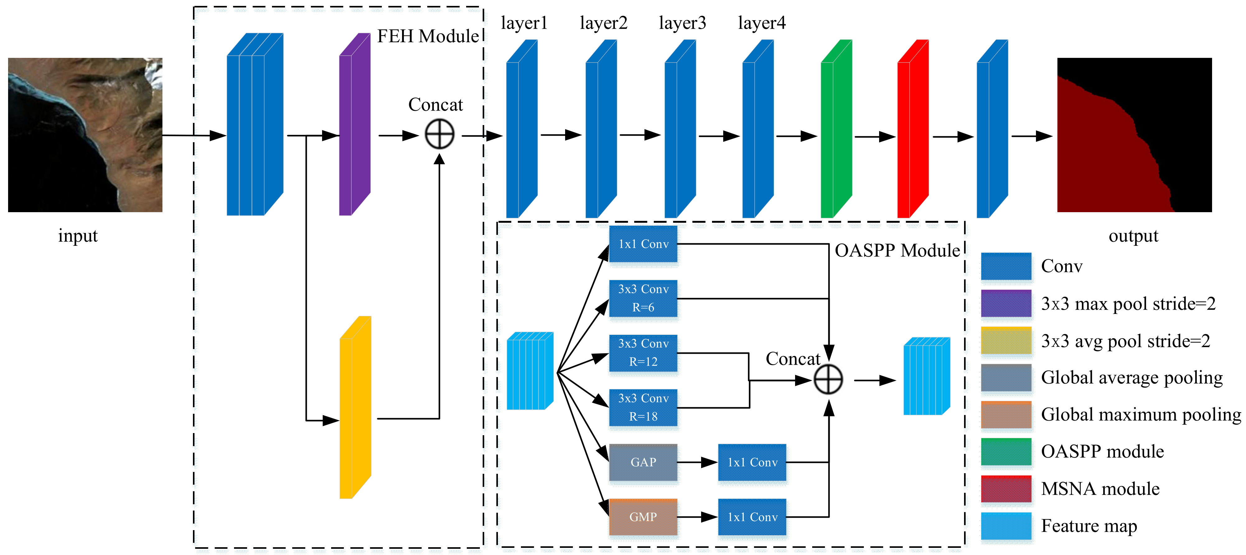
As depicted in Figure 2, MSNANet is based on an encoder–decoder framework. First of all, FEH is designed to enhance feature representation and diminish the indistinguishability. Simultaneously, it can significantly reduce training time and accelerate model convergence. Subsequently, the enhanced feature maps are fed into OASPP after four convolution layers. More specifically, the receptive fields of different sizes are integrated into OASPP to capture multiscale context information, which improves the accuracy and mapping ability of the model. Then, the encoded feature maps are fed into MSNA. It establishes long-distance feature dependencies between channels and realizes accurate fusions of multiscale context information. Finally, the resolution is reconstructed by convolution and upsampling, and the final segmentation result is output. The rest of this section will elaborate on MSNA, OASPP, and FEH modules in detail.

3.1. Multiscale Normalization Attention Module

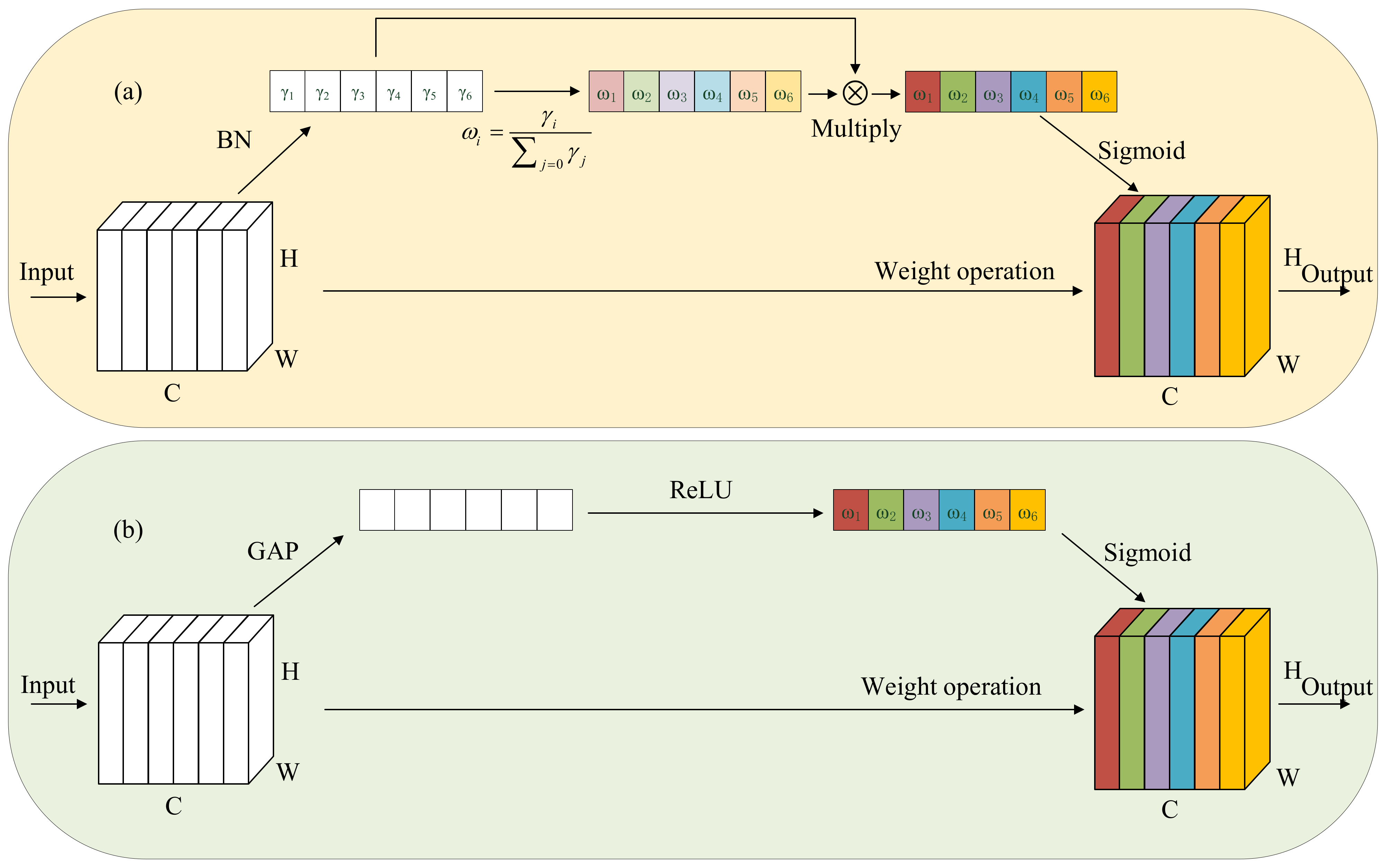
Inspired by Liu et al. [43], a multiscale normalization attention (MSNA) module was designed in this study. An MSNA module is an optimized channel attention mechanism which refines feature maps with well-rounded multiscale semantic information. Specifically, two primary components were designed and embedded: grouping strategy (GS) and normalization attention (NA) module (see Figure 3a). The input feature channels are equally divided into four groups in GS. Such a design enables the MSNA module to merge multiple pieces of multiscale semantic information and establishes long-distance feature dependencies, which can boost performance. The Squeeze-and-Excitation (SE) module represents the channel attention mechanism, recalibrating the channel-wise weights with correlations (see Figure 3b). Although competitive performance has been proven, the multiscale semantic information is neglected while compressing all the channel features into a single value. Thus, striving to address the aforementioned drawbacks, an NA module is proposed. Different to the way the SE module weighs feature maps, the NA module weighs and recalibrates feature maps with the learnable parameter γ , which is dynamically adapted during the training process. Consequently, the spatial information is preserved in the NA module. The weight of each feature map can be expressed as
W i = γ i 2 j = 0 γ j
where γ is the scale factor of each feature map after BN operation.
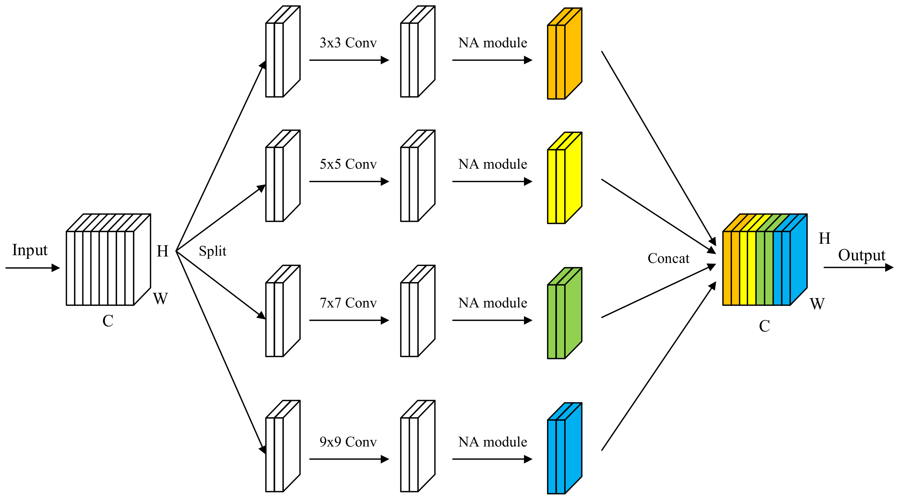
The pipeline of the MSNA module is illustrated in Figure 4. Firstly, the input feature maps are divided into four groups to establish the long-distance feature dependencies between channels. Subsequently, the convolution kernels of different sizes are operated on each group to extract multiscale context semantic information. Then, the low-level attention vectors of each group are obtained by BN operation. In our opinion, the low-level attention vectors are still limited and insufficient in channel feature representation. The low-level attention vectors are multiplied by γ to obtain high-level attention vectors. Ultimately, the feature maps are weighted by the high-level attention vectors and concatenated to obtain the final result.
The process can be described as follows:
[ X 0 ,   X 1 ,   ,   X S 1 ] = Split ( X )
F i = Conv ( K i × K i , G i ) ( X i ) , i = 0 ,   1 ,   ,   S 1
F = Concat ( [ F 0 ,   F 1 ,   ,   F S 1 ] )
where Split ( ) is the split operation, X is the number of the input channel, K i is the size of the convolution kernel, G i is the i-th group, F i is the convoluted feature map in the i-th group, Concat ( ) is the concatenate operation, and S is the number of the group.
On the basis of formula (7), the weights of feature maps in each group are obtained through the NA module (Figure 3a). The process is as follows:
Z i = σ ( W γ ( B N ( F i ) ) ) , i = 0 ,   ,   S 1
where Z i is the weight of feature maps in the i-th group, σ is the sigmoid function, W γ is the network weight, and B N ( ) is the BN operation.
Then, the feature maps are weighted by the attention vector:
Y i = F i Z i
where is the weighting channel operation and Y i is the weighted feature map in the i-th group.
Finally, the cross-channel information fusion is realized to obtain the final output:
Y = Y 0 Y 1 Y S 1
where is the group-merging operation.

3.2. Optimized Atrous Spatial Pyramid Pooling Module

In the field of computer vision, many scholars utilize ASPP extracting and fusing multiscale information to enhance the context understanding of the model [44,45,46,47,48,49,50]. Nevertheless, the high variation in water bodies (e.g., in terms of spectrum, geometry, and spatial size) is considered an essential factor affecting extraction accuracy. Furthermore, noise disturbances (such as mountain shadow) can easily cause misclassification in the model.
The ASPP module always consists of five branches, including one 1 × 1 convolution branch, three 3 × 3 convolution branches, and one global average pooling branch. Due to the limited sampling range and quantity of parallel branches, many valuable global features and context information cannot be fully sampled. The module performs favorably in extracting multiscale water bodies, being especially effective for large-scale water bodies, but it always fails to extract tiny water bodies (e.g., the RSI only includes a small part of tiny water areas) due to it is easily confusing water and background information during global average pooling. In this study, a global maximum pooling (GMP) branch has been integrated on the basis of ASPP, which can highlight the semantic features of tiny water bodies in the global receptive field (the structure can be seen in Figure 2). Firstly, 1 × 1 convolution was adopted to reduce the dimensions and provide more spatial details for the decoder. The 1 × 1 convolution branch allows tiny water body information to be preserved, which helps the model extract tiny water bodies. In addition, we utilized 3 × 3 convolution kernels with different dilated rates (r = 6, 12, 18) to obtain receptive fields of different sizes, which makes the multiscale features of water bodies more discernable. A relatively small dilated rate (r = 6) was used to extract small-scale water bodies. A relatively large dilated rate (r = 12, 18) was used to extract large-scale water bodies. Finally, GAP and GMP followed by a 1 × 1 convolution were integrated to realize global information interaction.
Simply put, OASPP not only captures rich multiscale detail information, but makes full use of global valuable information to suppress noise interference.

3.3. Head Module for Feature Enhancing

Different from the semantic segmentation of natural imagery, the semantic segmentation of RSI is extremely dependent on the representation ability of surface features. Affected by various factors, water bodies show dramatic variation in spectral features in RSI. This causes water bodies to be easily confused with other surface features, which decreases the segmentation ability of CNNs.
In this study, FEH (structure shown in Figure 2) was designed to improve feature distinguishability and accelerate network convergence. Firstly, a three-layer convolution operation was performed on the input to enrich the channel domain information. Subsequently, 3 × 3 average pooling and maximum pooling with a stripe of 2 were performed to compress the size of the input, which reduces the training time. More specifically, pooling operations can augment the representation of water body semantic features and discard the background information, which refines features for the following decoding stage. Ultimately, the pooled feature maps are concatenated to realize precise channel information interaction and feature injection.
In general, FEH provides enhanced semantic features for the decoder, which aid in performance.

4. Experiments

4.1. Dataset

In order to verify the performance and universality of MSNANet, extensive experiments were conducted on two public satellite remote sensing datasets: Surface Water dataset (SW dataset) and Qinghai–Tibet Plateau Lake dataset (QTPL dataset). The datasets contain more than 24,000 high-resolution RSIs of lakes in total, with different sizes and various shapes, with lakes in the shadows of clouds and water bodies connecting lakes (such as rivers).

4.1.1. Surface Water Dataset

The SW dataset is a novel visible spectrum satellite remote sensing dataset which includes three spectral bands—R (red), G (green), and B (blue)—and has annotated water bodies and backgrounds. The number of bits per pixel of each image is 24. There are 17,596 remote sensing images, 17,596 label images, and 17,596 visual label images in the original SW dataset, and the size is 256 × 256. Here, 80% of them were randomly assigned to the training set and 20% were assigned to the testing set, which are used for model training and testing, respectively. Finally, 14,077 training images and 3519 testing images were obtained.

4.1.2. Qinghai–Tibet Plateau Lake Dataset

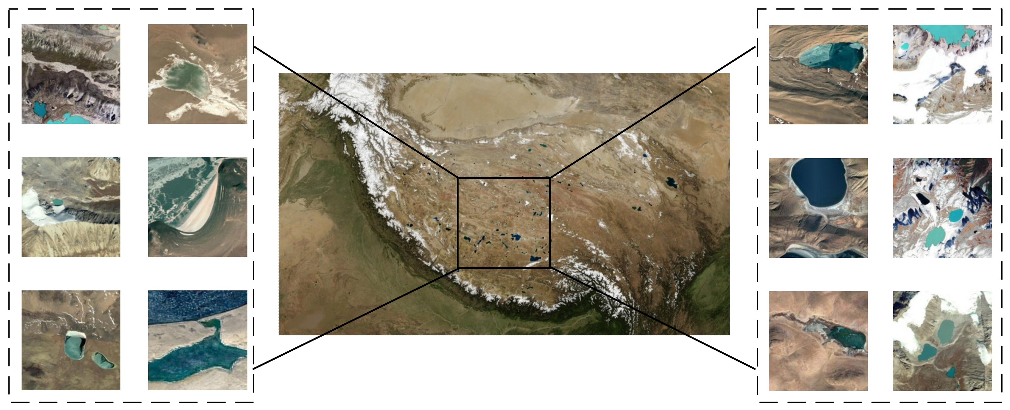
The QTPL dataset is a visible spectrum RSI dataset. Only lakes in the dataset are labeled by labelme [51]. The sampling location of the QTPL dataset is shown in Figure 5. There are 6774 remote sensing images in the QTPL dataset, with a size of 256 × 256. The number of bits per pixel of each image is 24, and the spatial resolution is 17 m. Here, 90% of them were randomly assigned to the training set and 10% were assigned to the testing set. Finally, 6069 training images and 705 testing images were obtained.
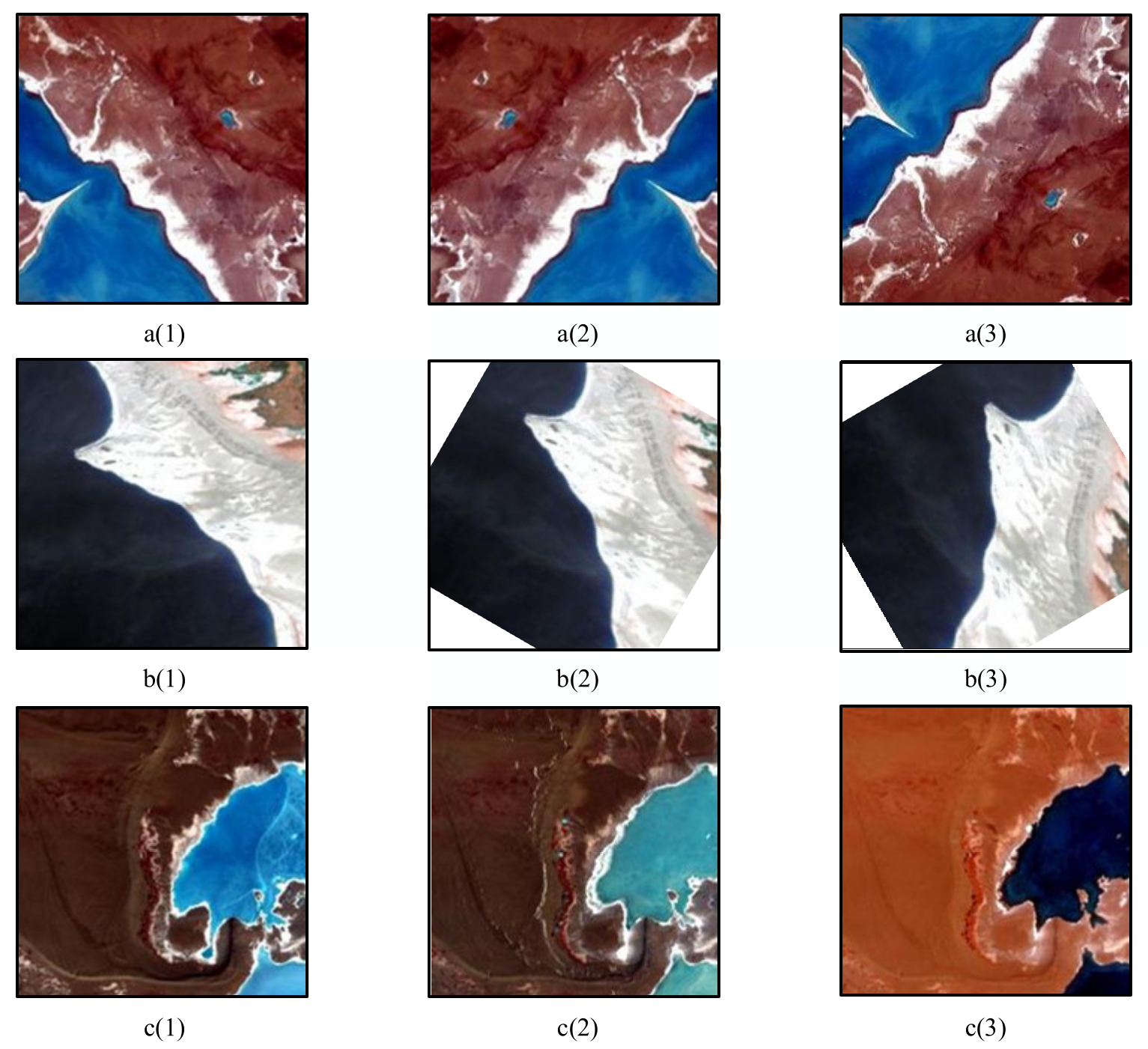
In an attempt to achieve superior performance and enhance the universality of the model, data augmentation—including random clipping, random horizontal sliding, random flipping, rotation, and color enhancement—was performed on all images before each epoch (Figure 6).

4.2. Experimental Details

The operating system used by the experiment was Ubuntu 20.04. The GPU was an NVIDIA Tesla V100 with 32 GB of memory. The deep learning framework used was Pytorch and the python version was Python 3.7. No models were pre-trained in the experiment. Before each epoch, all images were shuffled to enhance the generalization ability of the model. The batch size was set to 4. Cross entropy (CE) loss has been used as the loss function of the model; its formula is as follows:
H ( p , q ) = i = 1 n p ( x i ) log ( q ( x i ) )
where p ( x i ) and q ( x i ) are the true probability distribution and the predicted probability distribution, respectively. The goal of the training process is to minimize CE loss. In this study, the adaptive adadelta optimizer was adopted to update model parameters. The initial learning rate was set to 0.1. The learning rate reduction strategy can be calculated by the following formula:
l r = l r 0 × ( 1 e p o c h i e p o c h m a x ) 0.9
where l r is the current learning rate, l r 0 is the initial learning rate, e p o c h i is the current epoch, and e p o c h m a x is the maximum epoch (which was set to 200). The details regarding hyperparameters are listed in Table 1.

4.3. Evaluation Metrics

Essentially, extracting water bodies from RSI is a semantic segmentation task. Consequently, five semantic segmentation evaluation metrics were adopted to evaluate the performance of the proposed model: Overall Accuracy (OA), F1-score, kappa, Water Intersection over Union (WIoU), and Mean Intersection over Union (MIoU). The OA denotes the proportion of all correctly classified pixels to the total pixels. Ideally, both precision (P) and recall (R) should be as high as possible. When these two metrics are conflicting, it is difficult to evaluate the performance of the models. Therefore, in order to give consideration to both P and R, F1-score was adopted as the evaluation metric. Due to the imbalance between the number of water body pixels and background pixels in the dataset, the model is more inclined to predict pixels as the background pixels. In order to address the background bias of the model, kappa was introduced. The WIoU is the proportion of intersection and union of predicted water body values and real water body values, while the MIoU is the mean of intersection and union ratios of all categories; their formulae are as follows:
O A = T P + T N T P + T N + F P + F N × 100 %
F 1 - s c o r e = 2 1 p r e c i s i o n + 1 r e c a l l = 2 × p r e c i s i o n × r e c a l l p r e c i s i o n + r e c a l l × 100 %
p r e c i s i o n = T P T P + F P
r e c a l l = T P T P + F N
K a p p a = p 0 p e 1 p e
p 0 = O A = T P + T N T P + T N + F P + F N × 100 %
p e = ( T P + T N ) × ( T P + F P ) + ( F P + F N ) × ( T N + F N ) N 2
W I o U = T P F N + T P + F P × 100 %
M I o U = 1 k + 1 i = 0 k T P F N + T P + F P × 100 %
where TP denotes true positive. In this paper, this means the number of pixels correctly predicted to be water body pixels. FN denotes false negative. In this paper, this means the number of water body pixels incorrectly predicted to be background pixels. FP denotes false positive. In this paper, this means the number of background pixels incorrectly predicted to be water body pixels. TN denotes true negative. In this paper, this means the number of pixels correctly predicted to be background pixels.

4.4. Results and Analysis

To verify the performance of the proposed method, five advanced semantic segmentation models are presented in this section: DeeplabV3+ [10], SegNet [8], PSPNet [9], Attention U-Net [11], and LANet [52]. In addition, in order to verify the generalization ability of the proposed model, the experiments have been conducted on two datasets: Surface Water dataset and Qinghai–Tibet Plateau Lake dataset.

4.4.1. Results for the Surface Water Dataset

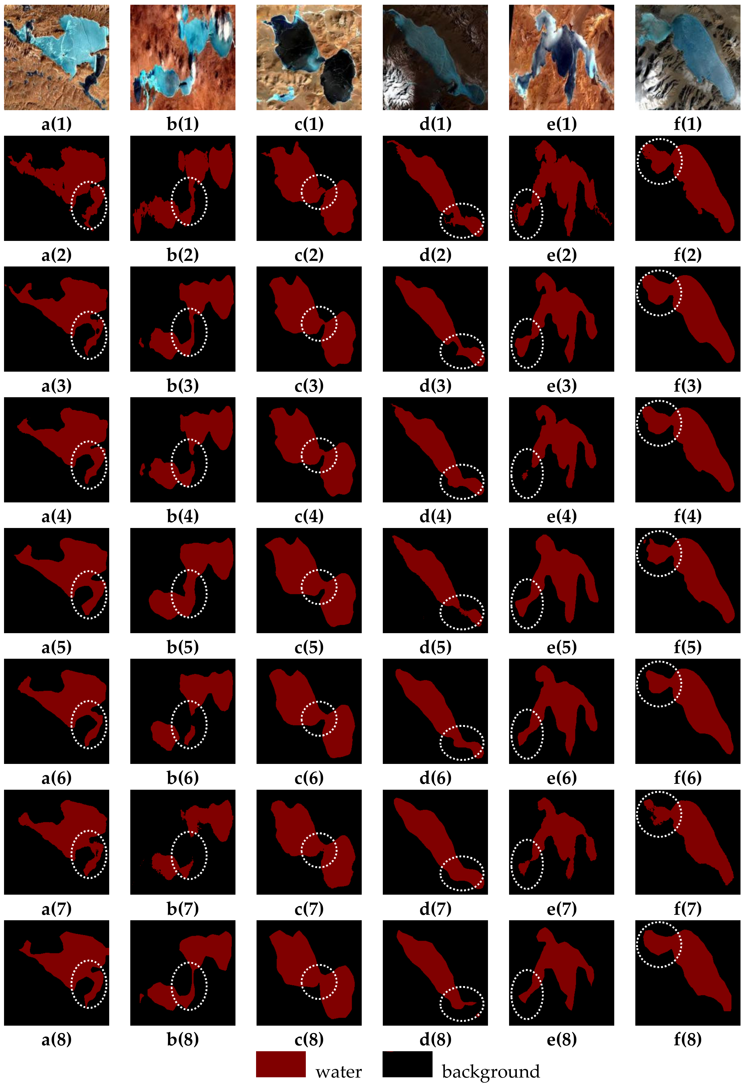
Quantitative comparison results for the SW dataset are summarized in Table 2. The boldface indicates the optimal result of each evaluation metric. It can be seen that MSNANet has outperformed others in five evaluation metrics: OA, F1-score, kappa, WIoU, and MIoU. The MIoU is 0.38% higher than the second best model, DeeplabV3+. Attention U-Net, which is also an embedded attention mechanism, is 1.1% lower than MSNANet in OA. LANet enhances feature representation by fusing high-level semantic information and low-level spatial information. Unfortunately, it is slightly problematic for the SW dataset. MSNANet achieved 92.12% and 0.87908 in F1-score and kappa, respectively, which indicates that MSNANet can better address the background bias. Visual inspections are shown in Figure 7, from which it can be seen that the proposed method can extract water bodies accurately in the narrow areas (a(3)–e(3)). In the case of cloud interference, it also performs better than other methods (b(1)–b(8)). This means MSNANet has a strong capability of resisting interference compared to other methods. When the spectral features of water bodies are quite different (a(1)–f(1)), MSNANet’s performance is not greatly affected. This means that the proposed method has a robust and stable extraction capability. The training time and the Flops (floating point operations) are listed in Table 3. Although the amount of parameters has increased, the computational time has not increased significantly, especially in the Flops. Meanwhile, the increased training time is acceptable. This means that the proposed method has good practicability while maintaining accuracy.

4.4.2. Results for the Qinghai–Tibet Plateau Lake Dataset

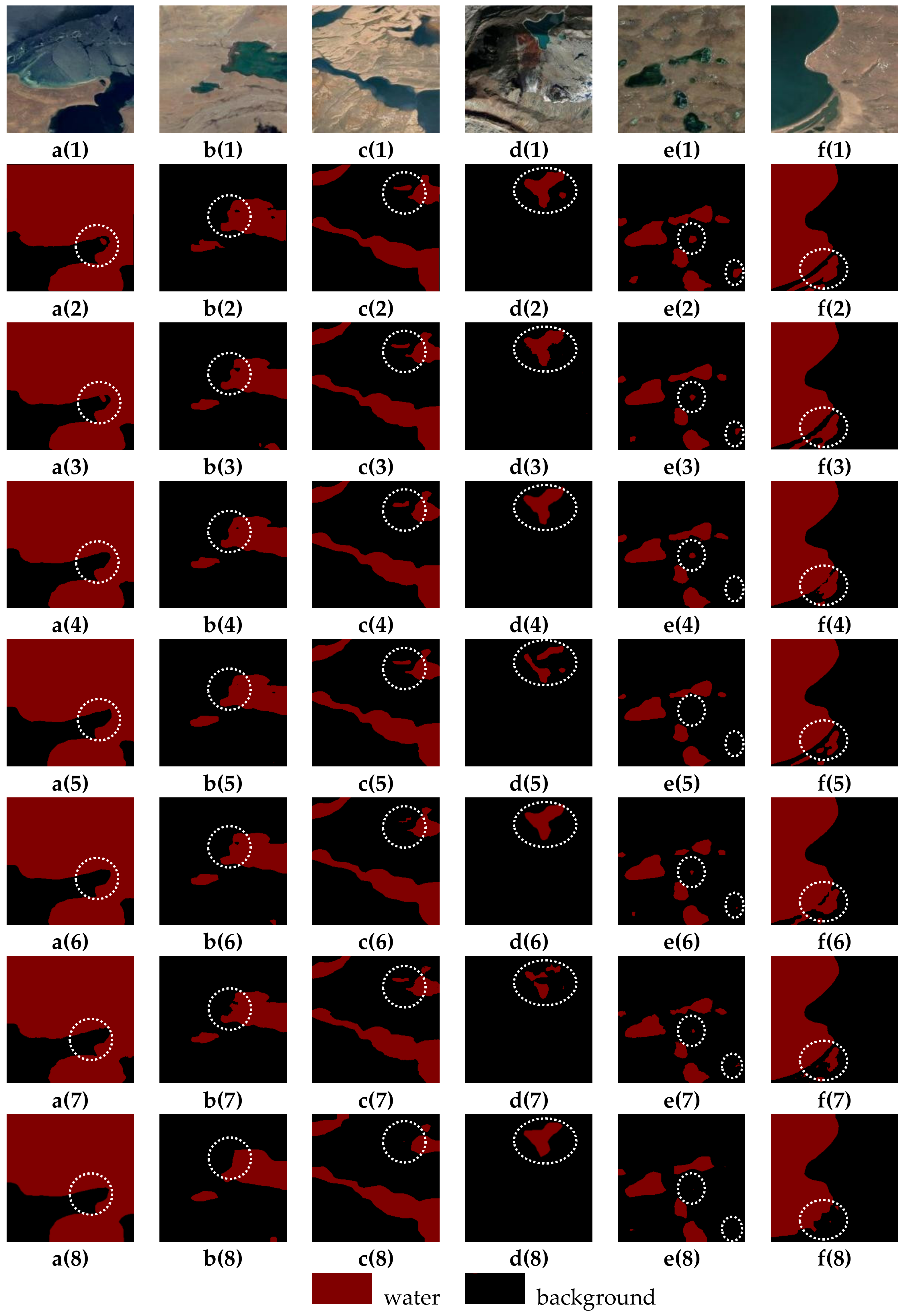
Quantitative comparison results for the QTPL dataset are summarized in Table 4. Statistically, the OA, F1-score, kappa, WIoU, and MIoU of MSNANet (98.47%, 98.11%, 0.96824, 96.29%, and 96.88%, respectively) are the highest. This sufficiently demonstrates MSNANet’s ability in feature discrimination and distinction perception. Figure 8 illustrates the visualization comparison for the QTPL dataset. Compared with other models, the inference result of MSNANet is the closest to the ground truth. In addition, MSNANet showed the best performance in water boundary prediction and anti-interference. As we can see, Attention U-Net is effective in extracting large water bodies, but fails to fully extract small water bodies (a(4), d(4), and e(4)). Compared with MSNANet, DeeplabV3+ showed better performance in extracting small water bodies, but it is vulnerable to shadows (d(5)). PSPNet has low water body extraction accuracy due to the use of multi-layer pooling operations (a(6)-e(6)), and the segmentation accuracy at water body boundaries is not very high (f(6)). SegNet is easily affected by shadows and its extraction accuracy is limited (a(7)–d(7)). LANet has some shortcomings in the extraction of small water bodies (a(8), c(8)–e(8)), and the delineation of water boundaries is not satisfactory (f(8)).

4.5. Ablation Study

In this section, the effectiveness of the proposed modules is analyzed comprehensively. In our strategy, the MSNA module was designed to extract multiscale water body features and enhance attention expression. The OASPP module was designed to extract multiscale context information and realize cross-scale feature interaction. The FEH module was designed to accelerate model training and increase feature distinguishability. In addition, in order to verify the universality of the proposed module, sufficient ablation experiments were performed on two datasets.
The statistical results of the ablation study are summarized in Table 5. For the SW dataset, after removing FEH, the OA, F1-score, kappa, WIoU, and MIoU decreased by 0.22%, 0.49%, 0.00694, 0.85%, and 0.61%, respectively. Meanwhile, the training time of each epoch increased by more than four-fold. After removing OASPP, the OA, F1-score, kappa, WIoU, and MIoU decreased by 0.11%, 0.21%, 0.00377, 0.36%, and 0.34%, respectively. Moreover, the amount of parameters decreased to 39.6 M. This means that OASPP introduces numerous parameters and computational burden while boosting the model performance, but the cost is acceptable. After ablation of MSNA, the OA, F1-score, kappa, WIoU, and MIoU decreased by 0.18%, 0.33%, 0.00527, 0.57%, and 0.47%, respectively, and the amount of parameters decreased by 1.7 M. The training time of per epoch did not increase significantly. Similar to the results for the SW dataset, the ablation study for the QTPL dataset also proved the performance of the proposed module. This means that the MSNA module does not introduce too much computational burden while improving the accuracy of the model. Consequently, we deem that the MSNA module is a lightweight and eminent channel attention module.
In order to verify the effectiveness of the proposed module visually, the segmentation result of the ablation study is shown in Figure 9. The visualization results show that when the FEH is removed, it is easy for the model to recognize the background as a water body, which impedes the classification ability (d(4), f(4)). Some tiny water bodies are missed when the OASPP is removed (a(5)–d(5)). After the ablation of MSNA, MSNANet has reduced capability in suppressing noise interference (c(5)). The error for water boundaries increased, which may lead to some areas being missed (b(6), d(6), e(6)).
In general, the quantitative and qualitative results of the ablation study demonstrate that each module we designed has preponderance in helping the model refine feature representation and optimize segmentation performance.

5. Conclusions

Along with the development of remote sensing technology, traditional water body extraction methods have deficiencies in automation scenes because they are affected by expert knowledge or artificial factors. In addition, the accuracy is limited because of the huge differences in water body spectral features, geometry, and spatial size. In order to address the above problems, MSNANet is proposed and implemented.
First of all, MSNA is designed to realize the attention interaction of multiscale water-body features. MSNA splits the input into four groups and extracts multiscale features with the convolution kernel of different sizes. Specially, MSNA weights feature maps according to the learnable parameter γ , which is learned by BN and dynamically adapted during the training process. Moreover, the OASPP we proposed concatenates multiscale features to realize cross-level information interaction and captures global valuable information for further performance improvement. Furthermore, FEH was designed to reduce training time and accelerate model convergence. Two parallel pooling branches were embedded in FEH to compress the size of the input and provide enhanced feature maps for the encoder.
Extensive experiments have been conducted for the SW dataset and QTPL dataset, and the results indicate the progressiveness of our strategy. Meanwhile, the ablation study utterly demonstrates the effectiveness of the modules we designed. MSNA is a novel lightweight and efficient attention module which can be flexibly applied to other computer vision scenes. In future work, the proposed method should be used and testified in different scenarios; in addition, the model structure should be evolved to capture the boundaries of water bodies more accurately.

Author Contributions

Conceptualization, X.L. (Xin Lyu) and Y.F.; methodology, Y.F.; software, Y.F.; validation, X.L. (Xin Lyu), Y.F. and B.T.; formal analysis, X.L. (Xin Li); investigation, Y.F. and X.L. (Xin Li); resources, X.L. (Xin Lyu), B.T., X.L. (Xin Li) and T.Z.; data curation, Y.F.; writing—original draft preparation, Y.F.; writing—review and editing, X.L. (Xin Lyu) and X.L. (Xin Li); visualization, Y.F.; supervision, X.L. (Xin Lyu); project administration, X.L. (Xin Lyu), B.T. and T.Z.; funding acquisition, X.L. (Xin Lyu) and B.T. All authors have read and agreed to the published version of the manuscript.

Funding

This research was funded by the Excellent Post-doctoral Program of Jiangsu Province (Grant No. 2022ZB166), Fundamental Research Funds for the Central Universities (Grant No. B210202080), and the Project of Water Science and Technology of Jiangsu Province (Grant No. 2021080).

Institutional Review Board Statement

Not applicable.

Informed Consent Statement

Not applicable.

Data Availability Statement

The datasets in our study are public. The Surface Water dataset can be found at https://aistudio.baidu.com/aistudio/datasetdetail/75148, (accessed on 24 August 2022). The Qinghai–Tibet Plateau Lake dataset can be found at http://www.ncdc.ac.cn/portal/metadata/b4d9fb27-ec93-433d-893a-2689379a3fc0, (accessed on 24 August 2022).

Conflicts of Interest

The authors declare no conflict of interest.

References

  1. Crétaux, J.F.; Abarca-del-Río, R.; Bergé-Nguyen, M. Lake Volume Monitoring from Space. Surv. Geophys. 2016, 37, 269–305. [Google Scholar] [CrossRef] [Green Version]
  2. Rokni, K.; Ahmad, A.; Selamat, A.; Hazini, S. Water Feature Extraction and Change Detection Using Multitemporal Landsat Imagery. Remote Sens. 2014, 6, 4173–4189. [Google Scholar] [CrossRef] [Green Version]
  3. Hamm NA, S.; Atkinson, P.M.; Milton, E.J. A per-pixel, non-stationary mixed model for empirical line atmospheric correction in remote sensing. Remote Sens. Environ. 2012, 124, 666–678. [Google Scholar] [CrossRef]
  4. McFeeters, S.K. The use of the Normalized Difference Water Index (NDWI) in the delineation of open water features. Int. J. Remote Sens. 1996, 17, 1425–1432. [Google Scholar] [CrossRef]
  5. Xu, H. Modification of normalised difference water index (NDWI) to enhance open water features in remotely sensed imagery. Int. J. Remote Sens. 2006, 27, 3025–3033. [Google Scholar] [CrossRef]
  6. Long, J.; Shelhamer, E.; Darrell, T. Fully Convolutional Networks for Semantic Segmentation. IEEE Trans. Pattern Anal. Mach. Intell. 2015, 39, 640–651. [Google Scholar]
  7. Ronneberger, O.; Fischer, P.; Brox, T. U-net: Convolutional networks for biomedical image segmentation. In Proceedings of the International Conference on Medical Image Computing and Computer-Assisted Intervention (MICCAI), Munich, Germany, 5–9 October 2015; pp. 234–241. [Google Scholar]
  8. Badrinarayanan, V.; Kendall, A.; Cipolla, R. Segnet: A deep convolutional encoder-decoder architecture for image segmentation. IEEE Trans. Pattern Anal. Mach. Intell. 2017, 39, 2481–2495. [Google Scholar] [CrossRef]
  9. Zhao, H.; Shi, J.; Qi, X.; Wang, X.; Jia, J. Pyramid Scene Parsing Network. In Proceedings of the IEEE Conference on Computer Vision and Pattern Recognition (CVPR), Honolulu, HI, USA, 21–26 July 2017; pp. 6230–6239. [Google Scholar]
  10. Chen, L.; Zhu, Y.; Papandreou, G.; Schroff, F.; Adam, H. Encoder-decoder with atrous separable convolution for semantic image segmentation. In Proceedings of the European Conference on Computer Vision (ECCV), Munich, Germany, 8–14 September 2018; pp. 801–818. [Google Scholar]
  11. Schlemper, J.; Oktay, O.; Schaap, M.; Heinrich, M.; Kainz, B.; Glocker, B.; Rueckert, D. Attention gated networks: Learning to leverage salient regions in medical images. Med. Image Anal. 2019, 53, 197–207. [Google Scholar] [CrossRef]
  12. Li, X.; Li, T.; Chen, Z.; Zhang, K.; Xia, R. Attentively Learning Edge Distributions for Semantic Segmentation of Remote Sensing Imagery. Remote Sens. 2022, 14, 102. [Google Scholar] [CrossRef]
  13. Miao, Z.; Fu, K.; Sun, H.; Sun, X.; Yan, M. Automatic Water-Body Segmentation from High-Resolution Satellite Images via Deep Networks. IEEE Geosci. Remote Sens. Lett. 2018, 15, 602–606. [Google Scholar] [CrossRef]
  14. He, C.; Li, S.; Xiong, D.; Fang, P.; Liao, M. Remote Sensing Image Semantic Segmentation Based on Edge Information Guidance. Remote Sens. 2020, 12, 1501. [Google Scholar] [CrossRef]
  15. Wang, B.; Chen, Z.; Wu, L.; Yang, X.; Zhou, Y. SADA-Net: A Shape Feature Optimization and Multiscale Context Information-Based Water Body Extraction Method for High-Resolution Remote Sensing Images. IEEE J. Sel. Top. Appl. Earth Obs. Remote Sens. 2022, 15, 1744–1759. [Google Scholar] [CrossRef]
  16. Weng, L.; Xu, Y.; Xia, M.; Zhang, Y.; Liu, J.; Xu, Y. Water areas segmentation from remote sensing images using a separable residual segnet network. ISPRS Int. J. Geo Inf. 2020, 9, 256. [Google Scholar] [CrossRef]
  17. Guo, H.; He, G.; Jiang, W.; Yin, R.; Yan, L.; Leng, W. A Multi-Scale Water Extraction Convolutional Neural Network (MWEN) Method for GaoFen-1 Remote Sensing Images. ISPRS Int. J. Geo Inf. 2020, 9, 189. [Google Scholar] [CrossRef] [Green Version]
  18. Zhang, X.; Xiao, Z.; Li, D.; Fan, M.; Zhao, L. Semantic Segmentation of Remote Sensing Images Using Multiscale Decoding Network. IEEE Geosci. Remote Sens. Lett. 2019, 16, 1492–1496. [Google Scholar] [CrossRef]
  19. Li, X.; Xu, F.; Xia, R.; Lyu, X.; Gao, H.; Tong, Y. Hybridizing Cross-Level Contextual and Attentive Representations for Remote Sensing Imagery Semantic Segmentation. Remote Sens. 2021, 13, 2986. [Google Scholar] [CrossRef]
  20. Wang, Z.; Gao, X.; Zhang, Y. HA-Net: A Lake Water Body Extraction Network Based on Hybrid-Scale Attention and Transfer Learning. Remote Sens. 2021, 13, 4121. [Google Scholar] [CrossRef]
  21. Zhang, Z.; Lu, M.; Ji, S.; Yu, H.; Nie, C. Rich CNN Features for Water-Body Segmentation from Very High Resolution Aerial and Satellite Imagery. Remote Sens. 2021, 13, 1912. [Google Scholar] [CrossRef]
  22. Xu, Y.; Du, B.; Zhang, L. Self-Attention Context Network: Addressing the Threat of Adversarial Attacks for Hyperspectral Image Classification. IEEE Trans. Image Process. 2021, 30, 8671–8685. [Google Scholar] [CrossRef]
  23. Xu, Y.; Ghamisi, P. Consistency-Regularized Region-Growing Network for Semantic Segmentation of Urban Scenes with Point-Level Annotations. IEEE Trans. Image Process. 2022, 31, 5038–5051. [Google Scholar] [CrossRef]
  24. Li, Y.; Shi, T.; Zhang, Y.; Chen, W.; Wang, Z.; Li, H. Learning deep semantic segmentation network under multiple weakly-supervised constraints for cross-domain remote sensing image semantic segmentation. ISPRS J. Photogramm. Remote Sens. 2021, 175, 20–33. [Google Scholar] [CrossRef]
  25. Xu, Y.; Du, B.; Zhang, L. Robust Self-Ensembling Network for Hyperspectral Image Classification. IEEE Trans. Neural Netw. Learn. Syst. 2022; early access. [Google Scholar]
  26. He, K.; Zhang, X.; Ren, S.; Sun, J. Deep Residual Learning for Image Recognition. In Proceedings of the 2016 IEEE Conference on Computer Vision and Pattern Recognition (CVPR), Seattle, WA, USA, 27–30 June 2016; pp. 770–778. [Google Scholar]
  27. Panboonyuen, T.; Jitkajornwanich, K.; Lawawirojwong, S.; Srestasathiern, P.; Vateekul, P. Semantic Labeling in Remote Sensing Corpora Using Feature Fusion-Based Enhanced Global Convolutional Network with High-Resolution Representations and Depthwise Atrous Convolution. Remote Sens. 2020, 12, 1233. [Google Scholar] [CrossRef] [Green Version]
  28. Li, Z.; Chen, X.; Jiang, J.; Han, Z.; Li, Z.; Fang, T.; Huo, H.; Li, Q.; Liu, M. Cascaded Multiscale Structure with Self-Smoothing Atrous Convolution for Semantic Segmentation. IEEE Trans. Geosci. Remote Sens. 2022, 60, 1–13. [Google Scholar] [CrossRef]
  29. Ma, B.; Chang, C. Semantic Segmentation of High-Resolution Remote Sensing Images Using Multiscale Skip Connection Network. IEEE Sens. J. 2022, 22, 3745–3755. [Google Scholar] [CrossRef]
  30. Bai, H.; Cheng, J.; Huang, X.; Liu, S.; Deng, C. HCANet: A Hierarchical Context Aggregation Network for Semantic Segmentation of High-Resolution Remote Sensing Images. IEEE Geosci. Remote Sens. Lett. 2022, 19. Article Sequence Number: 6002105. [Google Scholar] [CrossRef]
  31. Kyrkou, C.; Theocharides, T. EmergencyNet: Efficient Aerial Image Classification for Drone-Based Emergency Monitoring Using Atrous Convolutional Feature Fusion. IEEE J. Sel. Top. Appl. Earth Obs. Remote Sens. 2020, 13, 1687–1699. [Google Scholar] [CrossRef]
  32. Li, H.; Qiu, K.; Chen, L.; Mei, X.; Hong, L.; Tao, C. SCAttNet: Semantic Segmentation Network with Spatial and Channel Attention Mechanism for High-Resolution Remote Sensing Images. IEEE Geosci. Remote Sens. Lett. 2021, 18, 905–909. [Google Scholar] [CrossRef]
  33. Niu, R.; Sun, X.; Tian, Y.; Diao, W.; Chen, K.; Fu, K. Hybrid Multiple Attention Network for Semantic Segmentation in Aerial Images. IEEE Trans. Geosci. Remote Sens. 2022, 60, 1–18. [Google Scholar] [CrossRef]
  34. Li, R.; Zheng, S.; Duan, C.; Sun, J.; Zhang, C. Multistage Attention ResU-Net for Semantic Segmentation of Fine-Resolution Remote Sensing Images. IEEE Geosci. Remote Sens. Lett. 2022, 19. Article Sequence Number: 8009205. [Google Scholar] [CrossRef]
  35. Sinha, A.; Dolz, J. Multi-Scale Self-Guided Attention for Medical Image Segmentation. IEEE J. Biomed. Health 2021, 25, 121–130. [Google Scholar] [CrossRef] [Green Version]
  36. Li, X.; Xu, F.; Lyu, X.; Gao, H.; Tong, Y.; Cai, S.J.; Li, S.Y.; Liu, D.F. Dual attention deep fusion semantic segmentation networks of large-scale satellite remote-sensing images. Int. J. Remote Sens. 2021, 42, 3583–3610. [Google Scholar] [CrossRef]
  37. Ioffe, S.; Szegedy, C. Batch normalization: Accelerating deep network training by reducing internal covariate shift. In Proceedings of the International Conference on Machine Learning, Lille, France, 7–9 July 2015; pp. 448–456. [Google Scholar]
  38. Zeng, T.; Xu, F.; Lyu, X.; Li, X.; Wang, X.; Chen, J.; Wu, C. Feature difference for single-shot object detection. IET Image Process. 2022, 1–17. [Google Scholar] [CrossRef]
  39. Lin, G.; Milan, A.; Shen, C.; Reid, I. Refinenet: Multi-path refinement networks for high-resolution semantic segmentation. In Proceedings of the IEEE Conference on Computer Vision and Pattern Recognition (CVPR), Honolulu, HI, USA, 22–25 July 2017; pp. 1925–1934. [Google Scholar]
  40. Yu, Z.; Feng, C.; Liu, M.; Ramalingam, S. Casenet: Deep category-aware semantic edge detection. In Proceedings of the IEEE Conference on Computer Vision and Pattern Recognition (CVPR), Honolulu, HI, USA, 21–26 July 2017; pp. 5964–5973. [Google Scholar]
  41. Bertasius, G.; Shi, J.; Torresani, L. Deepedge: A multi-scale bifurcated deep network for top-down contour detection. In Proceedings of the IEEE Conference on Computer Vision and Pattern Recognition (CVPR), Boston, MA, USA, 8–10 June 2015; pp. 4380–4389. [Google Scholar]
  42. Xie, S.; Tu, Z. Holistically-nested edge detection. In Proceedings of the IEEE International Conference on Computer Vision (CVPR), Santiago, Chile, 13–16 December 2015; pp. 1395–1403. [Google Scholar]
  43. Liu, Y.; Shao, Z.; Teng, Y.; Hoffmann, N. NAM: Normalization-based Attention Module. arXiv 2021, arXiv:2111.12419. [Google Scholar]
  44. Bai, R.; Jiang, S.; Sun, H.; Yang, Y.; Li, G. Deep Neural Network-Based Semantic Segmentation of Microvascular Decompression Images. Sensors 2021, 21, 1167. [Google Scholar] [CrossRef]
  45. Zhang, C.; Jiang, W.; Zhao, Q. Semantic Segmentation of Aerial Imagery via Split-Attention Networks with Disentangled Nonlocal and Edge Supervision. Remote Sens. 2021, 13, 1176. [Google Scholar] [CrossRef]
  46. Li, L. Deep Residual Autoencoder with Multiscaling for Semantic Segmentation of Land-Use Images. Remote Sens. 2019, 11, 2142. [Google Scholar] [CrossRef] [Green Version]
  47. Wu, Y.; Jiang, J.; Huang, Z.; Tian, Y. FPANet: Feature pyramid aggregation network for real-time semantic segmentation. Appl. Intell. 2022, 52, 3319–3336. [Google Scholar] [CrossRef]
  48. Lian, X.; Pang, Y.; Han, J.; Pan, J. Cascaded hierarchical atrous spatial pyramid pooling module for semantic segmentation. Pattern Recognit. 2021, 110, 0031–3203. [Google Scholar] [CrossRef]
  49. Baheti, B.; Innani, S.; Gajre, S.; Talbar, S. Semantic scene segmentation in unstructured environment with modified DeepLabV3+. Pattern Recognit. Lett. 2020, 138, 223–229. [Google Scholar] [CrossRef]
  50. Yang, M.; Yu, K.; Zhang, C.; Li, Z.; Yang, K. DenseASPP for Semantic Segmentation in Street Scenes. In Proceedings of the 2018 IEEE Conference on Computer Vision and Pattern Recognition (CVPR), Salt Lake City, UT, USA, 18–23 June 2018; pp. 3684–3692. [Google Scholar]
  51. Wang, Z.; Gao, X.; Zhang, Y.; Zhao, G. MSLWENet: A Novel Deep Learning Network for Lake Water Body Extraction of Google Remote Sensing Images. Remote Sens. 2020, 12, 4140. [Google Scholar] [CrossRef]
  52. Ding, L.; Tang, H.; Bruzzone, L. LANet: Local Attention Embedding to Improve the Semantic Segmentation of Remote Sensing Images. IEEE Trans. Geosci. Remote Sens. 2021, 59, 426–435. [Google Scholar] [CrossRef]
Figure 1. Dilated convolution with different dilated rate r. (ac) are the dilated rates of 0, 1, and 2, respectively.
Remotesensing 14 04983 g001
Figure 2. The structure of MSNANet. Inside the dotted box are the structures of FEH and OASPP, respectively.
Remotesensing 14 04983 g002
Figure 3. Pipeline of (a) normalization attention (NA) module and (b) Squeeze-and-Excitation (SE) module. The white cubes represent the unweighted feature maps, and the colored cubes represent the weighted feature maps. Different colors represent different weights. Light-colored rectangles indicate the low-level attention vector, and dark-colored rectangles indicate the high-level attention vector.
Remotesensing 14 04983 g003
Figure 4. Pipeline of MSNA module. The white cube represents the unweighted feature maps, and the colored cubes represent the weighted feature maps. Different colors represent weighted feature maps with different scales.
Remotesensing 14 04983 g004
Figure 5. Sampling location of Qinghai–Tibet Plateau Lake dataset. Inside the dotted box are some typical samples.
Remotesensing 14 04983 g005
Figure 6. Data augmentation. a(1)a(3) random flipping, b(1)b(3) random rotation, c(1)c(3) color enhancement. The first column indicates the original image; the second and third columns indicate the enhanced image from the first column, respectively.
Remotesensing 14 04983 g006
Figure 7. Visualization results for the SW dataset: a(1)f(1), images; a(2)f(2), ground truth; a(3)f(3), MSNANet; a(4)f(4), Attention U-Net; a(5)f(5), DeeplabV3+; a(6)f(6), PSPNet; a(7)f(7), SegNet; a(8)f(8), LANet. The white circles indicate obvious differences.
Remotesensing 14 04983 g007
Figure 8. Visualization results for the QTPL dataset: a(1)f(1), images; a(2)f(2), ground truth; a(3)f(3), MSNANet; a(4)f(4), Attention U-Net; a(5)f(5), DeeplabV3+; a(6)f(6), PSPNet; a(7)f(7), SegNet; a(8)f(8), LANet. The white circles indicate obvious differences.
Remotesensing 14 04983 g008
Figure 9. Visualization results of ablation study: a(1)f(1), images; a(2)f(2), ground truth; a(3)f(3), MSNANet; a(4)f(4), MSNANet (without FEH); a(5)f(5), MSNANet (without OASPP); a(6)f(6), MSNANet (without MSNA). a(1)c(1)—images in the SW dataset; d(1)f(1)—images in the QTPL dataset. The white circles indicate obvious differences.
Remotesensing 14 04983 g009
Table 1. Details of hyperparameter settings.
HyperparameterSetting
Batch size4
Loss functionCross entropy loss
OptimizerAdadelta
Initial learning rate0.1
Maximum epochs200
Table 2. Quantitative comparison for the SW dataset. Bold numbers indicate the best results.
MethodOAF1-ScoreKappaWIoUMIoU
MSNANet94.4492.120.8790885.488.66
Attention U-Net93.3490.560.8547982.7686.54
DeeplabV3+94.391.870.8748784.9688.28
PSPNet94.1791.730.8729984.7288.12
SegNet94.1591.550.870184.4187.87
LANet94.1491.620.8711484.5287.96
Table 3. Comparison in terms of computational time. Bold numbers indicate the best results. The size of the input was 256 × 256.
MethodParams (M)Training Time (s)Flops (G)
MSNANet72.362761.943
Attention U-Net34.945966.636
DeeplabV3+54.734820.757
PSPNet46.841346.112
SegNet29.427140.169
LANet24.02558.309
Table 4. Quantitative comparison for the QTPL dataset. Bold numbers indicate the best results.
MethodOAF1-ScoreKappaWIoUMIoU
MSNANet98.4798.110.9682496.2996.88
Attention U-Net98.2497.870.9634795.7696.42
DeeplabV3+98.3998.030.9669196.1496.75
PSPNet98.498.030.967196.1596.77
SegNet98.1297.690.9613595.4996.21
LANet98.2997.890.9645795.8696.52
Table 5. Quantitative analysis of ablation study. Training time indicates the training time of each epoch. Bold numbers indicate the best results.
DatasetMethodParams (M)OAF1-ScoreKappaWIoUMIoUTraining Time (s/epoch)
SW datasetMSNANet72.394.4492.120.8790885.488.66627
MSNANet (without FEH)72.294.2291.630.8721484.5588.052629
MSNANet (without OASPP)39.694.3391.910.8753185.0488.32373
MSNANet (without MSNA)70.694.2691.790.8738184.8388.19611
QTPL datasetMSNANet72.398.4798.110.9682496.2996.88326
MSNANet (without FEH)72.298.3197.960.9658596.0196.651097
MSNANet (without OASPP)39.698.4198.050.9671396.1796.77157
MSNANet (without MSNA)70.698.3797.980.9662196.0696.68254
Publisher’s Note: MDPI stays neutral with regard to jurisdictional claims in published maps and institutional affiliations.