Article

Gravity Wave Parameters and Their Seasonal Variations Study near 120°E China Based on Na LIDAR Observations

1
College of Physics & Electronics Engineering, Hainan Normal University, Haikou 571158, China
2
State Key Laboratory of Space Weather, National Space Science Center, CAS, Beijing 100011, China
3
China-Brazil Joint Laboratory for Space Weather, CAS, Sao Jose dos Campos 12227-010, Brazil
4
Key Laboratory of Laser Technology and Optoelectronic Functional Materials of Hainan Province, Haikou 571158, China
5
National Institute for Space Research, INPE, São José dos Campos 12227-010, Brazil
6
Innovation Academy for Precision Measurement Science and Technology, CAS, Wuhan 430071, China
7
School of Science, Jiangsu University of Science and Technology, Zhenjiang 212003, China
8
College of Electronic Engineering, Nanjing Xiaozhuang University, Nanjing 211171, China
*
Author to whom correspondence should be addressed.
Remote Sens. 2022, 14(19), 4798; https://doi.org/10.3390/rs14194798
Submission received: 9 July 2022 / Revised: 3 September 2022 / Accepted: 15 September 2022 / Published: 26 September 2022
(This article belongs to the Special Issue Selected Papers of the European Lidar Conference)

Abstract

:
Based on the established LIDAR chain along the 120°E meridian in China, the gravity wave (GW) activity between 80 and 105 km and the seasonal behavior of temporal and spatial spectra at Beijing, Hefei and Hainan were studied with three years of continued observations. The averaged GW-induced atmospheric density perturbations are near 6%, which in summer are obviously larger than in winter. The semiannual maxima occur near the solstice and the minimum emerges around the equinox at different latitudes. Besides, as a disparity, the density perturbation of GW is still active considerably in winter at low latitude at Hainan. The spectra of vertical wave number Fa(m) and observed frequency Fa(ω) show power law shapes, of which the average is near −3 and −1.7, respectively, and both spectra with special values all exhibit similar seasonal behavior as the atmospheric density perturbations shows. This behavior is explained by multiple effects possibly originating from Tibet plateau (TP) and the main GW source in China was roughly calculated by the LIDAR observation method for the first time located at the TP boundary.

Graphical Abstract

1. Introduction

Gravity waves (GW) studies are significant contents of investigating the atmosphere structure and the middle large-scale circulation [1,2]. During the past decade, GW phenomena in the middle atmosphere have been studied extensively based on remote sensing and in situ techniques widespread. According to the superior temporal and spatial resolutions of LIDAR which are 3 min and 100 m, it is recognized as an excellent tracer of the sodium layer to study GW perturbations and the mesopause region [3,4,5,6]. It permits us to investigate several important characteristics of the wave field that until now have not been studied extensively, such as the atmosphere density perturbation, and temporal and spatial spectra based on the Na LIDAR data [7,8].
According to previous research, it is also quite important to acquire sodium layer data of the mesospause region, during which the detecting techniques are still not so sufficient up to now, and Na LIDAR has the advantage to detect these regions exclusively. And for GW seasonal distribution study, those observing results at the different observing site are usually different due to the complex geography factor, such as Senft and Gardner [8] has reported the maxima GW perturbation emerged at solstice and the minimum at equinox at north America, Yang et al. [7] has given an opposite observation report at Brazil that the maximum GW perturbation emerged at the two equinoxes and the minimum at solstices.
Despite the fact that a great deal of work has focused on the measurements of GW variances and their spectra, however, a comprehensive comparison of seasonal variation GW spectra studies at different latitudes over China is still rare until now. Moreover, due to the complex geographical factors of China’s mainland, such as large deserts, oceans and mountains, etc., from the north to the south of China, it exhibits diverse geographical environments, which will generate more different GW performances indeed. Moreover, vertical detection study of mesospause of China mainland is also seldom, the OH airglow detection only covers the flat region which cannot provide detailed information on GW in the vertical dimension. Furthermore, discussing the GW source of China’s mainland is a considerably hot topic in GW studies [9,10] currently. Therefore, for further understanding of generation mechanisms, resulting GW characteristics and the GW source position, starting the joint observation at different latitudes will provide long-term comparable research that is necessary and full of scientific meaning.
In this report, we use three comprehensive ground-based detecting LIDAR techniques to implement the initial whole-scale detection over China’s mainland. A comparable study of GW seasonal variations and their spectra parameters based on sodium LIDAR observation at China Beijing (40.42°N, 116.02°E), Hefei (31.8°N, 117.3°E) and Hainan (19.99°N, 110.34°E) which are near 120°E and based on the 3 year’s observation data by established “Meridian Project of China” [11,12,13] is carried out. Three sites for the seasonal variations of GW atmosphere density perturbations and spectra in mesospause were first reported. The seasonal variations of those GW spectra at three sites are also investigated, and some abnormal seasonal variations were found at the lower latitude of China in winter. We finally discussed the seasonal behavior of GW over China and give possible explanations, accordingly.

2. Method

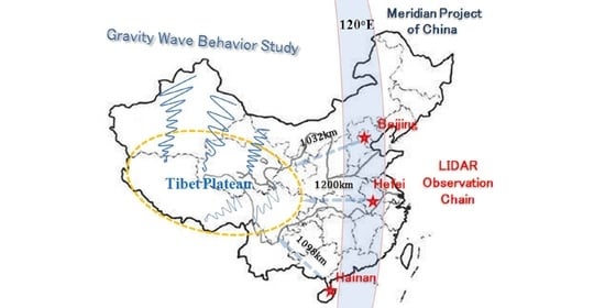
2.1. Instrumentations

As a part of the “Meridian Project”, the Na LIDARs at Hainan (19.99°N, 110.34°E), Hefei (31.8°N, 117.3°E) and Beijing (40.42°N, 116.02°E) employed the same double wavelengths sodium fluorescence LIDAR solution to observe the sodium layer. Besides, the Rayleigh and Mie scattering detection are also contained in the observatory system in which the laser beams were excited by a pulsed Nd: YAG laser.
The laser emission system: The laser emission system is composed as follows: First, a 1064 nm fundamental frequency light emitted by a high-power pulsed Nd: YAG laser passes through the first frequency multiplier to output 532 nm green light, and the remaining 1064 nm fundamental frequency light then passes through the second frequency multiplier. The second beam of 532 nm green light was obtained, which was used to pump a dye laser to produce the 589 nm laser. Therefore, this lidar system transmitted two laser beams: One is a 532 nm laser beam, which obtained 30–80 km atmosphere density and temperature, and atmosphere aerosol information from the ground to 30 km height by Rayleigh scattering mechanism. The other is a 589 nm beam, which obtained 80–110 km sodium density directly.
Telescope receiving system: The system is composed of two telescopes: a large telescope (1 m in diameter) is 5 m away from the emitting laser. Two optical fibers are placed side by side on the focal plane of this large telescope to receive 80–110 km of sodium layer signals and 30–80 km of atmospheric Rayleigh scattering signals, respectively. Another small telescope (0.4 m in diameter) is placed next to the laser beam and used to receive echo signals under 30 km. This signal can be used to calculate the extinction coefficient of the aerosol.
Signal Detection and Acquisition Channel: It is divided into three signal detection and acquisition channels. The sodium layer and atmospheric Rayleigh scattering channel are composed of PMT, amplifier and photon counter, respectively. PMT converts the photon signal into an electronic pulse signal, and then the photon counter counts the number of photons. The low-altitude channel uses the equipment fabricated by LICEL company for signal receiving and collecting. And system parameters are briefly listed in Table 1 as given below.
The green sodium laser beams’ energy is 40 mJ per pulse while Rayleigh and Mie scattering’s output energy is 400 mJ. To make the laser resonate well with sodium atoms in the neutral sodium layer between 85 and 105 km, we used a hollow cathode lamp to calibrate the sodium D2 frequency line as a standard. After the resonant fluorescence is received by a mirror 1000 mm diameter scale telescope. The altitude resolution has been set to about 96 m (while the altitude resolution at Hefei is 156 m according to the equipment parameters).
Our sodium LIDARs have an altitude resolution of 96 m (156 m at Hefei), and a time resolution of 3 min (5 min at Hefei). The data were selected from 2010 to 2012 in Beijing and Hainan and from 2006 to 2009 in Hefei which includes more than 160 observational nights and almost all the effective data are of good quality and have a continuous observation time of over 3 h. It is worth mentioning that we need to discard some data with the presence of sporadic sodium layers which are not generated by the gravity waves as reported by Batista et al. [14], (please see in the Supplementary Materials).

2.2. Data and Analysis Method

According to SG91 and more authors, Garner and Volez 1987, Garner and Shelton 1985, sodium layer is assumed as a Gaussian shape, and for Chemical effect and Sporadic Na layers, the Gaussian shape may be changed. Moreover, as we mention that around 94 km the severe dynamic activity happens change the Gaussian shape, those phenomena are of the nature of sodium layer, which are every often during every night observation. However, we need to filter these non-Gaussian effects to investigate the GW, since these issues affect the extract the perturbation of the Na layer.
Following the theory proposed by Senft and Gardner 1991 [8], in this report we calculated the atmosphere density perturbations that can be explicated during the temporal evolution of the density of sodium and atmosphere as indicated in Equation (1). The symbol rs(z, t) was used to express the perturbation of sodium density; thus ra(z, t) was defined as the perturbations of atmospheric density; and considering the effect of the unperturbed sodium layer, we use z0 and σ0 to denote the centric height (about 92 km) and their RMS thickness which is generally about 4.5 km, respectively.
r s ( z , t ) = 1 γ - 1 [ 1 γ H ( z z 0 ) σ 0 2 ] r a ( z , t )
where γ denotes the ratio of specific heats, H is atmosphere scale height which is about 6 km. According to Equation (1), the atmospheric density perturbation ra(z, t) can be obtained from the above relationship, Due to the existence of non-Gaussian shaped sodium layer distribution near 94 km, we need to discard some data near that altitude as it caused the severe fluctuation in calculating the ra(z, t). Technically the density perturbation relationship between atmosphere and sodium can be shortened as Equation (2) according to the previous studies of Yang et al., (2006) and Senft and Gardner (1991). In detail, when we do this we can see that the absolute value of the term in square brackets |Sca(z)| (here, we use Sca(z) to denote [1 − γH(z − z0)/σ2]) in Equation (2) will go to zero near the height z1 = z0 + σ2γH~94 km, and this means the first-order wave effects have no influence on the sodium profile in this height. As a result of this, it is not possible to get a reliable value of ra(z,t) from rs(z,t) within ± 2 km of z1 [8]. So, we have to discard some data points where |Sca(z)| is too small in math, the region is meaningless, and actually, in the Na layer, this height~94 km has severe perturbation and disorder chaos. Thus, the method we handle this problem is to discard the data around this region.
r a ( z , t ) = γ 1 1 γ H f ( z ) r s ( z , t )
where f (z) = − ρ 0 ( z ) / ρ 0 ( z ) . In practice, ρo (z) and f (z) were acquired by numerical calculation depend on the ρo(z) which of a Gaussian sodium layer shape that are unperturbed.
Perturbations studies of atmosphere density
The averaged square ra(z,t) are quite significant physical quantity in gravity wave analysis, in our section, a spatial and temporal calculus for the averaged rs(z,t) was done to obtain this value
< r a 2 ( z , t ) > = 1 T L z 0 L / 2 z 0 + L / 2 t - T / 2 t + T / 2   r a 2 ( z , t ) d t d z
where L’ is the altitude range, T is the whole night observation period. Similarly, in our analysis, those data points in the range of 2.5 km of z1 should be eliminated according to Yang et al. [7]. The temporal variations of <ra2> were then computed by averaging ra2 throughout the sodium layer over a period of T = 3 h.

3. Results

Figure 1 indicates the root mean square (RMS) atmospheric density perturbations, root <ra2(z,t)> for the sites at Beijing, Hefei and Hainan and their seasonal variation distribution. In this article, we use minimum mean square error (MMSE) fitting to calculate the components parameters of atmospheric density perturbation. And for brevity, we only show the fitted results here, while the fitting circumstances are given in detail in the Supplementary Materials.
As shown in Figure 1 (top), Seasonal variations in Beijing with their MMSE fit of the atmospheric density perturbations’ RMS value are 5.84% (see in Supplementary Materials), and the RMS values in summer are obviously larger than that in winter and the maxima occur near the solstice. While the semiannual minimal phase is near the equinoxes, and the contribution of annual perturbation is calculated and provided in Supplementary Materials. Compared to the similar latitude (Urbana, IL, USA) given by Senft and Gardner [8], this report also indicated that the annual maxima perturbations are near the solstices while the minima are around the equinoxes.
The seasonal variation RMS value of atmospheric density curves at low-middle (Hefei) and low latitude (Hainan) is also calculated as shown in Figure 1 (middle) and (bottom), both the seasonal variation exhibits a regulation overall as Beijing that maxima are near the solstices while minimum equinox which indicates that RMS perturbations at middle and low-middle latitude have the similar result seasonally. This result inferred that at the 120°E china the GW atmospheric density perturbations have the same regularity, which could be generated from the same GW source. According to the previous reports [9,10], TP affects most regions of China mainland and is the main GW source.
However, obviously, it worth mentioned that the perturbation in winter is still quite active at Hainan which may indicate there is another abnormal GW activity, which means at the low latitude region, the atmosphere density perturbation in winter has a relatively stronger activity compared with the middle latitude region’s regularity. Referring to the environment of the Hainan observatory at low latitudes near the South China Sea, there could be extra sources that cause the abnormal GW activities in winter due to the wind shear of the Tibetan plateau (TP) which will be discussed in a later chapter.

3.1. Study of Atmospheric Density Perturbations’ Vertical Wave Number Spectra

In order to investigate the GW field energies, the vertical wave number spectrum Fa(m) which is also called the vertical power spectrum is considered to be the effective method based on the analysis of the density of atmosphere perturbation. According to Gardner’s theory, Fa(m) is defined as the spatial Fourier transform of atmospheric density perturbations as [7,8].
F a ( m ) = B a ( s , 0 ) e i m s d s = < r a ( z , t ) · r a ( z s , t ) > e i m s d s
In the above functions, the autocorrelation function was represented by Ba(s, 0), which means the product of atmospheric density perturbations at adjacent height: <ra(z, t), ra(z−s, t)> which is appropriate for our work because the calculations will have no lack of data points as there is an 8 km large gap in the sodium layer. And we calculate all the spectra parameters for the vertical wave number spectrum and temporal frequency spectrum which can be seen in Supplementary Materials.
The seasonal variations of Fa(m) at three sites are shown in Figure 2, and special wavelengths was chosen for characterization with those parameters as m8 = 2π/(8 km), m4 = 2π/(4 km), m2 or m15 = 2π/(2 or 1.5 km) (while for Hefei and Hainan we choose m2 = 2π/(2 km) for instead) and m1 = 2π/(1 km) at three sites. For all the variations the maxima occur near the half of the year. The phases of the annual and the semiannual components are both near the solstice and their values are calculated as 39% and 27% of the annual mean value respectively. The other annual mean value of the specific spectra we choose is a correlation with the wavelength, as the variation value of Fa(m4) is 0.22 (m/cycles), which is only 26% of the variations Fa(m8). The ratio of annual components to the mean annual value of Fa(m4), Fa(m15), and Fa(m1) are 0.48, 0.61, and 0.60, respectively, which are all about 50%. That means these at-wave number contributions of the annual and semiannual components are similar. We also studied the Fa(m) and their fitting parameter based on the data at Hefei and Hainan. The relationship between parameters of m8~m1 exhibited a similar result as Beijing, and the minimum perturbation all occurs near equinoxes and the phase of variation peaks are also around the solstice. Their distribution of vertical wave numbers was shown in Figure 2 (middle) and (bottom) which indicated the similar regulation at Urbana as Senft and Gardner reported [8]. However, it is worth mentioning that the perturbation in winter, also as the seasonal variation of Fa(m) shows, is still quite active in Hainan which may indicate there is another abnormal GW activity in the previous studies as reported by Yang et al. [7] and Senft and Gardner [8] comparatively.

3.2. Study of Atmospheric Density Perturbations’ Temporal Frequency Spectra

Similarly, the GW perturbations also can be studied by investigating the temporal frequency spectra, Fa(ω). The data processing and spectra calculations are quite similar to the vertical wave number Fa(m). After the pre-whitening and Hamming window processing, Fa(ω) can be defined as
F a ( ω ) = B a ( 0 , τ ) e i ω τ d τ | R a ( z , ω ) | 2 T
which was also proposed by Senft and Gardner [8].
Similar to the GW vertical wave number spectra, we choose those periods at 60 min, 40 min, and 25 min to characterize the distribution of atmosphere density perturbation Their spectral amplitudes of three sites at ω1 = 2π/60 min (square), ω2 = 2π/40 min (circle), and ω3 = 2π/25 min (triangles)are shown in Figure 3. Obviously, all the Fa(ω) amplitudes variations are also coherent with the distribution of RMS atmosphere perturbation at three places.
It is worth mentioning that as shown in Figure 4 (bottom), in winter, the Fa(ω) amplitudes in Hainan are still strong relatively that cannot be neglected, and are quite different from the result we observed in Beijing and Hefei shown in Figure 1 (top) and (middle), although the specific frequencies show the similar result of the total density seasonal perturbation in which that maxima and minimum are also near the summer solstices and equinox, respectively.

3.3. GW Activity along the 120°E in China and Their Seasonal Variation Behaviors

3.3.1. Analyze GW Activity along 120°E in China and Their Seasonal Variation Studies

Determining the wave source is a focus topic in GW studies at current despite the numerous reports about GW source inferring studies. Here we use Senft and Gardner’s [8] theory to calculate the possible wave source position. The relationship between zonal and vertical background winds could be used to calculate the wave source, which is equal to
u w = ( g N ) 2 r a 2 g 2 N 4 ( r a t ) 2
where
( g N ) r a 2 = u 2
g 2 N 4 ( r a t ) 2 = w 2
u denotes as zonal background wind; w denotes vertical background wind; g represents gravity acceleration and N means Brunt-Vaissalla frequency.
Based on the above calculations, the horizontal distance between the observation site and the GW source could be obtained. Since the sodium layer peak is about 90 km on average, so we use this value as the vertical distance, and the distance between observing sites and wave source has been calculated as shown in Table 2.
The distance between the wave source and our observing site is 1098 (from Hainan), 1132 (from Beijing), and 1200 (from Hefei) as shown in Table 2, which are at a rough value at 1100 km. According to the topography map of China, the most possible region for the three observing sites’ wave sources located at the westward 120 °E observing monitor chain, are near the TP as Figure 4 indicated, which are most probably located at the edge of Tibetan Plateau. This result is consistent with previously reported, which suggested that the Tibetan could be the main important wave source.
Gong et al. [15], used the quasi-monochromatic statistics method to calculate the ratio of observation of GWs period and Brunt-Vaisala period and estimated the average distances between the main tropospheric sources and the observing sites are 3660 km, 3480 km, and 3800 km for Beijing, Hefei, and Hainan sites respectively, which is different from our result, since we use perturbation value of atmosphere analysis to calculate wave source that is also a different approach. And our result is consistent with the GW generated from the edge of TP which belongs to the GW topography fact mechanism. Wan et al. [10] have given a report on the vortexes for the central region of China by TIDs (traveling ionospheric disturbances), meanwhile statistically analyzing the exciting sources of the TIDs based on the HF Doppler array. The TIDs were observed dominant to be propagating from northeastward and southeastward directions of TP. The feedback signal indicated vortexes more likely generated near lee sides of the plateau which also means that the sources of northeastward and southeastward.
TIDs are located in the southeastern and northeastern edges of TP respectively. Moreover, the incidence of vortexes and the TID sources statistical seasonally are fitted well with regional distributions geographically, and the calculation from each site to the assumed wave source region is just at the bounder of the TP, which is quite consistent with our calculations about GW source positions that exist a rough distance of 1200 km westward to the 120°E observing chain. Meanwhile, a TEC (ionospheric total electron content) detection method was used by Xu et al. [9] who indicated numerous vortexes were generated near the edges of the plateau and propagated up to a much higher altitude based on the atmosphere dynamics investigation, which confirmed the main possible GW source of China mainland. While it fitted well when comparing our calculations with reports by Wan et al. [10] and Xu et al. [9], thus it is more likely that our result is reliable based on the above analysis.

3.3.2. Analysis of GW Activity in Beijing and Hefei and Their Seasonal Variation Studies

From the measured results, it can be concluded the GW activity near 120°E China has regularity as the GW activity in summer are obviously larger than that in winter. The maxima occur near the solstice and the semiannual minimum is near the equinoxes. Due to this regularity, we try to analyze the possible wave source as given below.
At first, it was well recognized that topography and convection are the main factors to generate GW [16,17,18] and the main wave source of China’s mainland is the TP [10]. Based on the above analysis, the GW seasonal variation activity in Beijing and Hefei indicates similar results to Urbana’s region located in North America as Senft and Gardner reported [8]. The atmospheric density perturbation and amplitudes of spatial and temporal density perturbation spectra all show a seasonal distribution with maxima variations emerging near the solstice.
To investigate the background winds in the mesosphere over Beijing and Hefei, we plotted in Figure 5 the mean zonal wind diagram for Northern China which can reflect the seasonal distribution of altitude–zonal wind relation based on the open mode model HWM93 (http://modelweb.gsfc.nasa.gov/ last access on 10 February 2015. in which we extract the open data and plotted diagram by ourselves) also considering the troposphere and lower stratosphere (TIS) behaviors in Beijing given by Zhang and Yi [19]. The zonal wind shows the obvious annual symmetry distribution that in spring and summer the horizontal background wind is westward but mainly eastward from September to the next February. While considering the temperature effect, it is well known that in China the temperature of the atmosphere at lower altitudes in summer is a maximum and more GWs will be generated due to the strong and frequent convection considering the significant influence of TP that is located at the southwest direction. Moreover, considering the mean westward zonal wind above Northern China opposes the background wind, those GW northeastward propagated from the TP to Beijing and Hefei will be enhanced due to the Doppler filtering effect, which will lead to relatively strong GW atmosphere perturbations. Moreover, Gong et al. [15,20], once reported this conclusion; TP is the main GW source in china. although Gong’s work [20] indicated that the annual behavior of the event number of GW and their seasonal distribution is similar to our result, however, the essence of GW property is totally different, in this manuscript, we use atmosphere perturbation intensity to study GW, which directly indicated the GW behavior of an intrinsic dynamic motions demonstration rather than the GW events statistics.
While in winter, much fewer GWs will be generated from the TP because of the minimum cold atmosphere temperature which would cause relatively weak convections. Furthermore, when GWs propagate northeastward from the TP to Beijing in winter, the blocking effects will happen due to the eastward mean zonal background wind. Consequently, as being blocked by the mean flow during the obliquely upward propagations, the GWs could dissipate and be absorbed and finally, most of them are disappeared. This result is more reasonable to explain that the atmosphere density perturbation has a relatively weaker behavior in winter. Based on the above analysis, the reason for seasonal variation can be concluded as the reaction of the topography of TP and the convection.

3.3.3. Analysis of the Seasonal Variation of Gravity Wave Activity in Hainan

Obviously, however, the GWs seasonal variation activity in China, Hainan, shows quite different behavior in the latter half of the year. The activity in winter is still strong which cannot be neglected, referring to the topography of Hainan, there is a presence of a complex ocean current and frequent convection in the South China Sea at relatively lower latitude, so there may be another wave source that caused the different seasonal variations there. Though references suggest that the ocean effect is important to affect China’s mainland’s convection, according to our fitting results, the three places in Beijing, Hefei, and Hainan are very uniform, and their uniform behavior is that the summer is large, and the winter is small. This is also consistent with the results of Urbana in the land area of the United States. According to geographies, the ocean has little influence on the Urbana of the United States, the GW behavior in the Urbana area is not the role of the ocean. The waveforms found in the three places in China are highly consistent with Urbana, and it is believed that the influence of the ocean is also limited. Moreover, the oceanic action in the Pacific region is very strong in late summer and autumn, including tropical cyclones from the equatorial latitudes and so on. Therefore, the atmospheric perturbations in summer and autumn in Hefei, mid-latitude, or low-latitude Hainan should be very severe, and there will not be great regular perturbations during the mid-year summer solstice. Thus, the main one is from the action of mountain waves. Meteorological literature also shows that the convection in the western Pacific Ocean in summer can indeed affect the China mainland [21,22,23,24,25]. At the same time, the convection and ocean temperature effect from the equatorial latitude can interact mutually to form a large-scale Ocean-Atmosphere Circulation, which has been confirmed. However, this convection from the ocean even did not affect the regular distribution of Beijing and Hefei, which has the same regularity as Hainan, also the South China Sea convection affection is not very clear, and that intensive convection is much more effective when located in the equator. Alexander et al. [26] and Wright [27] reported that the momentum flux of GW of the South China Sea became minimum during the Monsoon period. And they were mainly caused by the intense and frequent convection from the South China Sea, which is an important region that generates ascending cyclones globally [26,27]. However, this explanation is weak, and according to the climatology in Hainan, winter from November to January is the dry season in Hainan, and there is seldom severe convection, such as typhoons or storms. Therefore, there should be some other GW source in Hainan in winter.
As indicated by Li et al. [28], in the winter, the GWs propagation directions at China-Qujing station (located at the strait line of Haikou and TP) are southeastward, which are significantly different from another observatory in the northern hemisphere. Analyzed by seasonal variation of the GW propagation, this propagation direction was proved accordingly. Meanwhile, the wind shear intensity is large around the southeastern edge of the TP in spring and winter based on European Centre for Medium-Range Weather Forecasts (ECMWF) reanalysis wind data. When more active GWs generated at TP edge, due to the Doppler shift effect, in winter the southeastward propagation of those GWs is enhanced by the northwestward background wind, the GW propagation directions affected by the background winds are stronger and momentum fluxes present a strong seasonal variation, with the maximum in winter and minimum in summer. The above analyzed GWs behaviors matched well with our results, however, these airglow image observations are different from LIDAR detection, to further understand the low latitude GWs activity of China, more technique and joint observations are needed in future.

4. Conclusions

The seasonal variation of GW activity at three different sites in Beijing, Hefei, and Hainan near 120°E China was measured based on three years of observation. The RMS atmosphere perturbation, the vertical wave number spectral amplitudes at 2π/(8 km) 2π/(4 km) 2π/(2 km), and 2π/(1 km) and ω spectra with those frequencies as 2π/60 min, 2π/40 min, 2π/25 min indicated that solstices are dated, around which the maxima of semiannual peaks and components emerge, while in Hainan the GW activity in winter is still active, which is quite different from Hefei and Beijing in the middle latitude region. The vertical wave number spectra and frequency spectra at different sites were calculated to be fitted well with the theoretical value. It is concluded that the fact of the TP’s topography could be the main reason for GW’s behavior at 120°E. The main possible gravity wave source caused by TP that influences China’s mainland was first estimated by the LIDAR observation method, which was located near the Plateau edge after calculation, consistent with previous reports.

Supplementary Materials

The following supporting information can be downloaded at: https://www.mdpi.com/article/10.3390/rs14194798/s1, Table S1: Fitted Components of GW Parameters at Beijing at Annual and Semiannual; Table S2: Annual and Semiannual Components of Gravity Wave Parameters at Hefei; Table S3: Annual and Semiannual Components of Gravity Wave Parameters at Hainan; Figure S1: Selected Fa(m) and their fitting slope to the nightly spectra of GW atmospheric density perturbations nightly at Beijing; Figure S2: Vertical wave number power spectra of atmospheric density perturbations associated with gravity waves in the menopause region at Hefei; Figure S3: Frequency spectra of atmospheric density perturbations associated with gravity waves in the menopause region at Hainan; Figure S4: Annual averaged Fa(m) at Beijing, Hefei and Hainan; Figure S5: Distribution of the fitted regression spectra slopes Fa(m) at Beijing, Hefei and Hainan; Figure S6: Selected Fa(ω) and their fitting slope to the spectra of GW atmospheric density perturbations nightly at Beijing. The straight dotted lines are the regression fits to the spectra; Figure S7: Frequency spectra Vertical wave number power spectra of atmospheric density perturbations associated with gravity waves in the menopause region at Hefei; Figure S8: Frequency spectra of atmospheric density perturbations associated with gravity waves in the menopause region at Hainan; Figure S9: Annual averaged Fa(ω) and their linear regression fits at Beijing, Hefei and Hainan. Figure S10: Distribution of fitting slopes of Fa(ω) at Beijing, Hefei and Hainan in statistical seasonally [7,8,14,29,30,31,32,33,34].

Author Contributions

Conceptualization, X.Z. and G.Y.; methodology, X.Z., G.Y., J.W., T.Z., L.D. and X.C.; software, J.J. and H.Y.; validation, X.Z., G.Y., P.P.B. and V.F.A.; formal analysis, X.Z. and G.Y.; investigation, X.Z. and G.Y.; data curation, J.J., P.P.B. and V.F.A.; writing—original draft preparation, X.Z., G.Y. and Z.W.; writing—review and editing, X.Z., G.Y. and Y.X.; supervision, G.Y. and P.P.B.; project administration, X.Z. and G.Y.; funding acquisition, X.Z. and G.Y. All authors have read and agreed to the published version of the manuscript.

Funding

This work is financially supported by NSFC 62063005, 41564006, 41264006, 40905012 and 41174129, 41474130 and the Natural Science Foundation provide by Hainan Province No. 121RC535, 20164163. Youth Innovation Promotion Association of Chinese Academy of Sciences (2019150), Project of Stable Support for Youth Team in Basic Research Field, Chinese Academy of Sciences (Grant No. YSBR-018), Innovation Promotion Association of Chinese Academy of Sciences (2019150).

Data Availability Statement

All the data comes from the data center for Meridian Space Weather Monitoring Project (http://data.meridianproject.ac.cn/ (accessed on 12 August 2022)).

Acknowledgments

We thank Project Supported by the Specialized Research Fund for State Key Laboratories for financial support. And all data come from the data center for Meridian Space Weather Monitoring Project (http://data.meridianproject.ac.cn/ (accessed on 12 August 2022)). China-Brazil Joint Laboratory for Space Weather, and the Support by the International Partnership Program of Chinese Academy of Sciences. Grant No. 183311KYSB20200003. Here we give our special thanks to them all.

Conflicts of Interest

The authors declare no conflict of interest.

References

  1. Alexander, M.; Pfister, L. Gravity wave momentum flux in the lower stratosphere over convection. Geophys. Res. Lett. 1995, 22, 2029–2032. [Google Scholar] [CrossRef]
  2. Fritts, D.C.; Alexander, M.J. Gravity wave dynamics and effects in the middle atmosphere. Rev. Geophys. 2003, 41, 1003. [Google Scholar] [CrossRef]
  3. Gardner, C.S.; Voelz, D.Z. Lidar studies of the nighttime sodium layer over Urbana, Illinois, 2. Gravity waves. J. Geophys. Res. 1987, 92, 4673–4693. [Google Scholar] [CrossRef]
  4. Yang, G.; Clemesha, B.; Batista, P.; Simonich, D. Improvement in the technique to extract gravity wave parameters from lidar data. J. Geophys. Res. 2008, 113, D19111. [Google Scholar] [CrossRef]
  5. Yang, G.; Clemesha, B.; Batista, P.; Simonich, D. Lidar study of the characteristics of gravity waves in the mesopause region at a southern low-latitude location. J. Atmos. Sol. Terr. Phys. 2008, 70, 991–1011. [Google Scholar] [CrossRef]
  6. She, C.Y.; Yu, J.R.; Huang, J.W.; Nagasawa, C.; Gardner, C.S. Na temperature lidar measurements of gravity wave perturbations of wind, density and temperature in the mesopause region. Geophys. Res. Lett. 2012, 18, 1329–1331. [Google Scholar] [CrossRef]
  7. Yang, G.; Clemesha, B.; Batista, P.; Simonich, D. Gravity wave parameters and their seasonal variations derived from Na lidar observations at 23°S. J. Geophys. Res. 2006, 111, D21107. [Google Scholar] [CrossRef]
  8. Senft, D.C.; Gardner, C.S. Seasonal variability of gravity wave activity and spectra in the mesopause region at Urbana. J. Geophys. Res. 1991, 96, 17229–17264. [Google Scholar] [CrossRef]
  9. Xu, G.; Wan, W.; She, C.; Du, L. The relationship between ionospheric total electron content (TEC) over Ease Asia and the tropospheric circulation around the Qinghai-Tibet Plateau obtained with a partial correlation method. Adv. Space Res. 2008, 42, 219–223. [Google Scholar] [CrossRef]
  10. Wan, W.; Yuan, H.; Ning, B.; Liang, J.; Ding, F. Traveling ionospheric disturbances associated with the tropospheric vortexes around Qinghai-Tibet Plateau. Geophys. Res. Lett. 1998, 25, 3775–3778. [Google Scholar] [CrossRef]
  11. Wang, C. New Chains of Space Weather Monitoring Stations in China. Space Weather 2010, 8, S08001. [Google Scholar] [CrossRef]
  12. Li, H.; Wang, C.; Peng, Z. Solar wind impacts on growth phase duration and substorm intensity: A statistical approach. J. Geophys. Res. 2013, 118, 4270–4278. [Google Scholar] [CrossRef]
  13. Sun, T.R.; Wang, C.; Wang, Y. Different Bz response regions in the nightside magnetosphere after the arrival of an interplanetary shock: Multipoint observations compared with MHD simulations. J. Geophys. Res. 2012, 117, A05227. [Google Scholar]
  14. Batista, P.P.; Clemesha, B.R.; Batista, I.S.; Simonich, D.M. Characteristics of the sporadic sodium layers observed at 23°S. J. Geophys. Res. 1989, 94, 15349–15358. [Google Scholar] [CrossRef]
  15. Gong, S.; Yang, G.; Dou, X.; Xu, J.; Chen, C.; Gong, S. Statistical study of atmospheric gravity waves in the mesopause region observed by a lidar chain in eastern china. J. Geophys. Res. Atmos. 2015, 120, 7619–7634. [Google Scholar] [CrossRef]
  16. Long, R.R. Some aspects of the flow of stratified fluids, III, Continuous density gradients. Tellus 1955, 7, 341–357. [Google Scholar] [CrossRef]
  17. Sato, K. Small-scale wind disturbances observed by the MU radar during the passage of typhoon Kelly. J. Atmos. Sci. 1993, 50, 518–537. [Google Scholar] [CrossRef]
  18. Sato, K. A statistical study of the structure, saturation and sources of inertio-gravity waves in the lower stratosphere observed with the MU radar. J. Atmos. Terr. Phys. 1994, 56, 755–774. [Google Scholar] [CrossRef]
  19. Zhang, S.D.; Yi, F. Latitudinal and seasonal variations of inertial gravity wave activity in the lower atmosphere over central China. J. Geophys. Res. 2007, 112, D05109. [Google Scholar] [CrossRef]
  20. Gong, S.H.; Yang, G.T.; Xu, J.Y.; Wang, J.H.; Guan, S.; Gong, W.; Fu, J. Statistical characteristics of atmospheric gravity wave in the mesopause region observed with a sodium lidar at Beijing, China. J. Atmos. Sol. Terr. Phys. 2013, 97, 143–151. [Google Scholar] [CrossRef]
  21. Lee, D.Y.; Ahn, J.B.; Yoo, J.H. Climate dynamics Enhancement of seasonal prediction of East Asian summer rainfall related to western tropical Pacific convection. Clim. Dyn. 2015, 45, 1025–1042. [Google Scholar] [CrossRef] [Green Version]
  22. Huang, R.; Sun, F. Impacts of the tropical western Pacific on the East Asia summer monsoon. J. Meteorol. Soc. Jpn. 1992, 70, 243–256. [Google Scholar] [CrossRef]
  23. Huang, G. An index measuring the interannual variation of the East Asian summer monsoon—The EAP index. Adv. Atmos. Sci. 2004, 21, 41–52. [Google Scholar] [CrossRef]
  24. Lee, S.S.; Lee, J.Y.; Ha, K.J.; Wang, B.; Schemm, J. Deficiencies and possibilities for long-lead coupled climate prediction of the western North Pacific-East Asian summer monsoon. Clim. Dyn. 2011, 36, 1173–1188. [Google Scholar] [CrossRef]
  25. Li, C.; Lu, R.; Dong, B. Predictability of the western North Pacific summer climate demonstrated by the coupled models of ensembles. Clim. Dyn. 2012, 39, 329–346. [Google Scholar] [CrossRef]
  26. Alexander, M.J.; Gille, J.; Cavanaugh, C.; Coffey, M.; Craig, C.; Eden, T.; Francis, G.; Halvorson, C.; Hannigan, J.; Khosravi, R.; et al. Global estimates of gravity wave momentum flux from High Resolution Dynamics Limb Sounder observations. J. Geophys. Res. 2008, 113, D15S18. [Google Scholar]
  27. Wright, C.J.; Gille, J.C. HIRDLS observations of gravity wave momentum fluxes over the monsoon regions. J. Geophys. Res. 2011, 116, D12103. [Google Scholar] [CrossRef]
  28. Li, Q.; Xu, J.; Liu, X.; Yuan, W.; Chen, J. Characteristics of mesospheric gravity waves over the southeastern Tibetan Plateau region. J. Geophys. Res. 2016, 121, 9204–9221. [Google Scholar] [CrossRef]
  29. Beatty, T.J.; Hostetler, C.A.; Gardner, C.S. Lidar observations of gravity wave and their spectra near the mesopause and stratopause at Arecibo. J. Atoms. Sci. 1992, 49, 477–496. [Google Scholar] [CrossRef]
  30. Collins, R.L.; Nomura, A.; Gardner, C.S. Gravity waves in the upper mesosphere over Antarctica: Lidar observations at the South Pole and Syowa. Geophys. Res. Lett. 1994, 99, 5475–5485. [Google Scholar] [CrossRef]
  31. Dewan, E.M.; Good, R.E. Saturation and the ‘‘universal spectrum for vertical profiles of horizontal scalar winds in the atmosphere. J. Geophys. Res. 1986, 91, 2742–2748. [Google Scholar] [CrossRef]
  32. Dewan, E.M. The saturated-cascade model for atmospheric gravity wave spectra and the wavelength-period (W-P) relations. Geophys. Res. Lett. 1994, 21, 817–820. [Google Scholar] [CrossRef]
  33. Hines, C.O. The saturation of gravity waves in the middle atmo-sphere, part22. Development of Doppler-spread theory. J. Atmos. Sci. 1991, 48, 1360–1379. [Google Scholar]
  34. Tsuda, T.; Inoue, T.; Fritts, D.C.; Vanzandt, T.E.; Kato, S.; Sato, T.; Fukao, S. MST radar observations of a saturated gravity wave spectrum. J. Atmos. Sci. 1989, 46, 2440–2447. [Google Scholar] [CrossRef]
Figure 1. Seasonal variations of the RMS atmospheric density perturbations with their MMSE fit at Beijing (top), Hefei (middle) and Hainan (bottom).
Remotesensing 14 04798 g001aRemotesensing 14 04798 g001b
Figure 2. Seasonal variations of Fa(m) and their MMSE fits at Beijing (top), Hefei (middle) and Hainan (bottom).
Remotesensing 14 04798 g002aRemotesensing 14 04798 g002b
Figure 3. Distribution of variations of Fa(ω) statistical seasonally and their MMSE fit at 2π/60 min, 2π/40 min, and 2π/25 min. in Beijing (top), Hefei (middle), and Hainan (bottom).
Remotesensing 14 04798 g003aRemotesensing 14 04798 g003b
Figure 4. Diagram of evaluated GW source position located at the edge of TP.
Remotesensing 14 04798 g004
Figure 5. The mean horizontal wind diagram of Northern China.
Remotesensing 14 04798 g005
Table 1. System parameters of the multiple channel lidar system.
TransmitterNd: YAG LaserDYE Laser
Wavelength532 nm589 nm
Pulse energy400 mJ40 mJ
Repetition rate30 Hz30 Hz
Pulse width10 ns10 ns
Beam divergence<0.5 mrad<0.5 mrad
Receiver
Telescope aperture1 m
Field of view1 mrad
Bandwidth1.0 nm
Data acquisition
MCS-pci count rate150 MHz
Bin width640 ns
Table 2. The calculated distances between the observed site and wave source.
HainanBeijingHefei
Distance to wave source (km)109811321200
Publisher’s Note: MDPI stays neutral with regard to jurisdictional claims in published maps and institutional affiliations.

