Abstract
Conventional calibration methods used in hydrological modelling are based on runoff observations at the basin outlet. However, calibration with only runoff often produces reasonable runoff but poor results for other hydrological variables. Multi-variable calibration with both runoff and remote sensing-based evapotranspiration (ET) is developed naturally, due to the importance of ET and its data availability. This study compares two main calibration schemes: (1) calibration with only runoff (Scheme I) and (2) multi-variable calibration with both runoff and remote sensing-based ET (Scheme II). ET data are obtained from three remote sensing-based ET datasets, namely Penman–Monteith–Leuning (PML), FLUXCOM, and the Global Land Evaporation Amsterdam Model (GLEAM). The aforementioned calibration schemes are applied to calibrate the parameters of the Distributed Hydrology Soil Vegetation Model (DHSVM) through ε-dominance non-dominated sorted genetic algorithm II (ε-NSGAII). The results show that all three ET datasets have good performance for areal ET in the study area. The DHSVM model calibrated based on Scheme I produces acceptable performance in runoff simulation (Kling–Gupta Efficiency, KGE = 0.87), but not for ET simulation (KGE < 0.7). However, reasonable simulations can be achieved for both variables based on Scheme II. The KGE value of runoff simulation can reach 0.87(0.91), 0.72(0.85), and 0.75(0.86) in the calibration (validation) period based on Scheme II (PML), Scheme II (FLUXCOM), and Scheme II (GLEAM), respectively. Simultaneously, ET simulations are greatly improved both in the calibration and validation periods. Furthermore, incorporating ET data into all three Scheme II variants is able to improve the performance of extreme flow simulations (including extreme low flow and high flow). Based on the improvement of the three datasets in extreme flow simulations, PML can be utilized for multi-variable calibration in drought forecasting, and FLUXCOM and GLEAM are good choices for flood forecasting.
1. Introduction
Hydrological models are a critical tool for hydrological processes’ simulation and their behavior prediction, which are very important for water resource planning and management. Hydrological models, especially physically-based ones, contain dozens and even hundreds of parameters [1]. However, it is difficult to determine some parameters in hydrological models, owing to the complex actual environment and limited data [2,3]. Thus, parameter calibration is a necessary step in hydrological model implementation [4,5].
Hydrological models are usually calibrated against runoff observations at a few locations or only at the basin outlet. Calibration with only runoff does not guarantee acceptable simulation for other hydrological components, such as evapotranspiration and soil moisture [6,7,8]. Moreover, calibration with only runoff often results in parameter equifinality [9]. One way to address the aforementioned issues is to calibrate the model with multiple variables, such as runoff, evapotranspiration, soil moisture, and land surface temperature within the basin [10,11].
Among the abovementioned variables, evapotranspiration is a good choice to calibrate the hydrological models together with runoff, due to its importance in the water cycle, carbon cycle, and energy cycle [12,13]. However, the accurate observation of evapotranspiration remains lacking, owing to the complex terrain environment. Fortunately, remote sensing technology has greatly promoted the estimation of evapotranspiration in the past few decades [14,15,16]. The emergence of various regional or global evapotranspiration datasets is critical for ungauged and poorly gauged regions [17]. For example, the spatial–temporal characteristics of evapotranspiration over the Amazon River Basin remain largely uncertain, due to the sparse observation network and relatively short observational period of eddy covariance data. Thus, Wu et al. [18] assessed the reliability of five global remote sensing ET datasets (JUN10, ZEN14, ZHA15, ZHA16, and GLEAM) (besides GLEAM, the names of the datasets are composed of the name of the first author and the publication year of the references) over the Amazon River Basin, and the results revealed that JUN10 has the best performance for the magnitude at both site level and basin scale. Moreover, Paca et al. [19] merged six global ET datasets (Atmosphere–Land Exchange Inverse Model (MOD16), CSIRO Moderate-Resolution Imaging Spectroradiometer (MODIS) Reflectance-Based Evapotranspiration (CMRSET), Operational Simplified Surface Energy Balance (SSEBop), Surface Energy Balance System (SEBS), Atmosphere–Land Exchange Inverse (ALEXI), and GLEAM) to obtain an ensemble prediction of evapotranspiration rates for the complex and inaccessible environment of the Amazon River Basin.
With the rapid development of remote sensing-based ET datasets, it is worthwhile to investigate whether hydrological model performance can be improved when evapotranspiration is incorporated with runoff in multi-variable calibration. Recently, some studies have assessed the utility of remote sensing-based ET datasets in improving hydrological model performance [20]. Sirisena et al. [8] used the GLEAM ET dataset and measured the streamflow at four stations to calibrate the Soil and Water Assessment Tool (SWAT) for Chindwin Basin, Myanmar. The result shows that reasonable simulations for both streamflow and evapotranspiration were obtained in multi-variable calibration, but good performance could only be found in the corresponding variable (streamflow/ET) in single-variable calibration, and not for the other variable (ET/streamflow). Herman et al. [7] adopted two remote sensing-based ET datasets (SSEBop and ALEXI) into multi-variable calibration together with runoff, and the result revealed that the performance of ET simulation was improved, and runoff simulation was maintained in multi-variable calibration. Rajib et al. [21] compared several parameter calibration techniques, including calibration with only runoff, calibration with runoff and remote sensing-based ET data, and calibration with runoff and spatially distributed remote sensing-based ET data, and the results demonstrated that incorporating ET datasets into multi-variable calibration was indeed able to improve ET simulation and maintain runoff simulation.
As there are various remote sensing-based ET datasets, it is difficult to select a suitable ET dataset incorporated into multi-variable calibration for a specific region, which seriously affects hydrological model performance. Different ET datasets have different characteristics, even within a specific study area, owing to the diverse remote sensing input datasets and diverse ET estimate models emphasizing different physical and physiological controlling factors [22,23,24]. Therefore, it is still meaningful to evaluate the effect of incorporating various remote sensing-based ET datasets into the multi-variable calibration of hydrological models. In this study, three datasets are selected, namely FLUXCOM, GLEAM, and PML. These datasets have been widely used, and their accuracy has been evaluated in many regions. As for FLUXCOM, this dataset was obtained via machine learning to merge energy flux measurements from FLUXNET eddy covariance towers with remote sensing and meteorological data [22]. The use of FLUXNET lays the foundation for the accuracy of the FLUXCOM dataset. Furthermore, Tramontana et al. [25] evaluated the accuracy of FLUXCOM with observation-based data around the world and they revealed that the performance of FLUXCOM is very good. As for GLEAM, Yang et al. [26] evaluated its accuracy via eight sites from the Chinese Flux Observation and Research Network (ChinaFlux), and it achieved reasonable performance. The PML dataset has high accuracy when compared with ground observations from 95 global flux stations located across the globe [27,28,29]. In several studies, the GLEAM dataset has been applied in parameter calibration, and they obtained acceptable performance for both runoff and ET simulations [8]. Nevertheless, fewer studies have investigated the utility of PML and FLUXCOM in the multi-variable calibration of hydrological models. Furthermore, ET simulation has a greater impact on runoff simulation in humid regions than dry regions [24]. Additionally, the performance of low flow, intermediate flow, and high flow simulations based on multi-variable calibration with both runoff and ET is also worth exploring, and it is substantial for flood and drought forecasting.
This study aims to (1) evaluate the accuracy of three selected remote sensing-based ET datasets (namely PML, GLEAM, and FLUXCOM) against in situ observations of pan evaporation; (2) investigate the utility of remote sensing-based ET datasets for improving hydrological model performance (runoff and ET simulations) in multi-variable calibration (Scheme II) by comparing them to those from calibration with only runoff (Scheme I); (3) explore the performance of low flow, intermediate flow, and high flow simulations based on Scheme II. To this end, this paper is structured as follows: Section 2 describes the study area and data sources. The description of the methodology for this study is presented in Section 3. Section 4 provides the results and discussion, and the conclusions are summarized in Section 5.
2. Study Area and Data
2.1. Study Area
The Jinhua River is a tributary of the Qiantang River and is located in the midwestern region of Zhejiang Province, East China (Figure 1). The length of this river is 195 km and its catchment area above the Jinhua discharge station (control station) is 5996 km2 [30]. The Jinhua River Basin is subject to an Asian monsoon climate, which is characterized by abundant precipitation and high temperatures in summer and a rainless, cold winter. The annual mean temperature is 17 °C. Based on fifty years (1962–2011) of precipitation data, the annual mean precipitation is 1404.9 mm and is unevenly distributed, with more than 50% of annual rainfall falling from May to July [31]. The uneven distribution of precipitation has led to frequent floods and droughts. Solid hydrological simulation can provide support to disaster prediction and prevention, and water resource management.
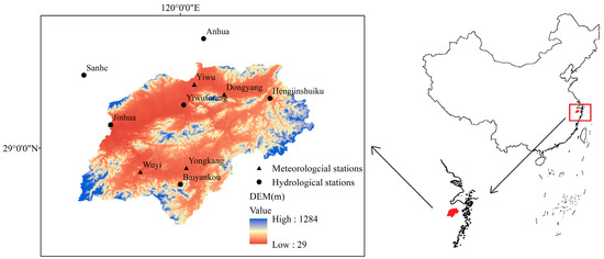
Figure 1.
The Jinhua River Basin and location of meteorological and hydrological stations used in this study.
2.2. Data Sources
2.2.1. In Situ Observations
The daily in situ observations used in this study are collected from six hydrological stations provided by the Zhejiang Provincial Hydrology Administration Center, and five meteorological stations obtained from the Zhejiang Provincial Meteorological Administration. The data period is 2004–2010. Six hydrological stations have records of daily pan evaporation, measured by E601 pan. Five meteorological stations have complete records of maximum and minimum air temperature, relative humidity, wind speed, sunshine duration, and precipitation. Since actual evaporation data are not available, the in situ observations of pan evaporation are used as the reference to evaluate the accuracy of remote sensing-based ET datasets. The in situ observations of meteorological data are used for hydrological model meteorological inputs.
2.2.2. PML
The PML-V2 dataset is provided for the period from July 2002 to December 2017, using the Google Earth Engine [27,28,29]. The dataset was derived from the MODIS dataset (leaf area index, albedo, and emissivity) together with Global Land Data Assimilation System (GLDAS) meteorological forcing data. The dataset includes gross primary product (GPP), soil evaporation (Es), vegetation transpiration (Et), and vaporization of intercepted rainfall (Ei). The ET from PML-V2 is the sum of Es, Et, and Ei. The PML-V2 dataset is provided on a 500-m spatial resolution with 8-day temporal resolution. The GPP and ET estimates obtained from PML-V2 have proven to be satisfactory when they are compared with measurements across 95 globally distributed flux sites [27,28,29]. In this study, the 500-m and 8-day PML-V2 dataset from 2004 to 2010 is used and can be freely downloaded (https://data.tpdc.ac.cn/zh-hans/data/48c16a8d-d307-4973-abab-972e9449627c/, accessed on 11 December 2020).
2.2.3. FLUXCOM
The FLUXCOM dataset is acquired via machine learning to merge energy flux measurements from FLUXNET eddy covariance towers with remote sensing and meteorological data to estimate global gridded net radiation, latent and sensible heat, and their uncertainties [22,32,33]. The FLUXCOM dataset includes two types of forcing data, i.e., 0.0833° resolution using a MODIS remote sensing dataset (RS), and 0.5° resolution using remote sensing and meteorological data (RS + METEO). Nine machine learning methods and three energy balance correction methods were utilized for RS forcing data. Three machine learning methods, three energy balance correction methods, and four global climate datasets were adopted for RS + METEO forcing data [22,32]. In this study, daily RS + METEO-based ensemble latent heat energy with 0.5° resolution from 2004 to 2010 that includes all fluxes produced by all energy balance correction methods, all machine learning methods, and all global climate datasets is used and can be freely downloaded (http://www.fluxcom.org, accessed on 21 December 2020). Latent heat flux divided by latent heat of vaporization is ET.
2.2.4. GLEAM
Central to the methodology of the GLEAM dataset is the use of the Priestley and Taylor evaporation model [34]. The dataset consists of four modules, namely the evaporation of intercepted rainfall from forest canopies, the water budget distributing the incoming precipitation (rain and snow) over the root zone, the stress conditions parameterized as a function of the root-zone available water and dynamic vegetation information, and the evaporation from each of the three surface components [23,34]. The GLEAM_v3.3b dataset is utilized in this study, which is provided on a 0.25° × 0.25° latitude–longitude grid with a daily temporal resolution. Actual ET in GLEAM is estimated as the sum of different ET components, including transpiration, interception loss, bare soil evaporation, snow sublimation, and open water evaporation. In this study, the daily GLEAM_v3.3b dataset with 0.25° resolution from 2004 to 2010 is used and can be freely downloaded (https://www.gleam.eu/, accessed on 30 November 2020).
3. Methodology
3.1. Model Setup
The DHSVM model is a fully distributed, physically based hydrological model that can provide an integrated representation of hydrology–vegetation dynamics at the spatial resolution represented by a digital elevation model (DEM) [35,36,37]. In this study, the spatial resolution is 200 m and the temporal resolution is daily. Version 3.1.1 of this model is adopted in this study.
The DEM is used to separate the river basin into computational grid cells. The model offers simultaneous solutions to water and energy balance equations in each grid cell and represents physical processes, including evapotranspiration, snowpack accumulation and snowmelt, canopy snow interception and release, unsaturated moisture movement, saturated subsurface flow, surface flow, and channel flow. Evapotranspiration is simulated by a two-layer canopy model and estimated by the Penman–Monteith equation. Because snow is very rare in the Jinhua River Basin, modules concerning snow, such as canopy snow interception and release, and snowpack accumulation and snowmelt, are not considered in this study. DHSVM uses Darcy’s law to control unsaturated moisture movement with multiple root-zone soil layers. A cell-by-cell method is adopted in DHSVM to route saturated subsurface flow using a kinematic or diffusion approximation. In this study, the explicit cell-by-cell approach is used for surface flow, i.e., surface runoff from each grid cell is first accumulated to the streams, and then routed downstream based on the stream network using the linear reservoir method (channel flow). DHSVM has been successfully applied in many research fields, including urbanization [38], climate change [30,39], and stream temperature simulations [40].
The input data for the hydrological model include meteorological and hydrological data (mentioned in Section 2.1), DEMs, masks (watershed boundary), vegetation and soil data, soil depth, and stream networks. The DEM data (90 m) are downloaded from the Shuttle Radar Topography Mission (SRTM) website (http://srtm.csi.cgiar.org/, accessed on 25 April 2016). The resolution of DEM is redefined to 200 m to reduce the computational burden. The mask is generated based on DEM. The vegetation data are obtained from WESTDC Land Cover Datasets 2.0 (2006) (http://westdc.westgis.ac.cn, accessed on 20 April 2016). The soil data are obtained from the Nanjing Institute of Soil Research, China. Because DHSVM uses the US Department of Agriculture (USDA) soil texture classification system, the soil classes are then reclassified. The soil depth and stream network are generated based on the mask and DEM by using Arc Workstation software.
3.2. Model Calibration
Model calibration is carried out through ε-NSGAII, which has been coupled with DHSVM by developing an automatic calibration model (εP-DHSVM) in the authors’ previous study [41]. Daily time series of runoff from the Jinhua hydrological station and three remote sensing-based ET datasets including PML, FLUXCOM, and GLEAM are used for parameter calibration and validation. Based on the data availability, all observed time series data are divided into calibration (2004–2008) and validation (2009–2010) periods.
Four different model calibration schemes are used to realize the aims (mentioned in the last paragraph of Section 1) of this study: (1) Scheme I—parameter calibration with only runoff; (2) Scheme II (PML)—parameter calibration using both runoff and ET based on PML dataset (ETPML); (3) Scheme II (FLUXCOM)—parameter calibration using both runoff and ET based on FLUXCOM dataset (ETFLUXCOM); (4) Scheme II (GLEAM)—parameter calibration using both runoff and ET based on GLEAM dataset (ETGLEAM).
In Scheme I, the KGE and percentage of relative bias (PBIAS) of runoff are used as objective functions. In all three variants of Scheme II, both KGE and PBIAS of runoff and ET are used as objective functions. Moreover, the performance of calibrated and validated results is also assessed with other evaluation indices, such as mean bias (ME), root mean square error (RMSE), and Pearson’s correlation coefficient (R).
The parameters used for model calibration are based on the two-step global sensitivity analysis results of DHSVM at the Jinhua River Basin [30]. Eight highly sensitive parameters, shown in Table 1, are used for model calibration in this study. Detailed procedures of the two-step global sensitivity analysis are omitted here, and interested readers can refer to [30].

Table 1.
Range, meaning, unit, and abbreviation of eight highly sensitive parameters for parameter calibration.
3.3. Evaluation Indices
Multiple statistical indices are used to evaluate the accuracy of the three remote sensing-based ET datasets and their performance in improving hydrological model performance. These indices include R, PBIAS, ME, RMSE, and KGE [42,43]. The five indices are defined as follows:
For assessing the accuracy of the three sensing-based ET datasets, and in the above equations denote in situ observations and remote sensing-based ET datasets, respectively. and are the mean values of these two datasets, respectively. For KGE, is the linear correlation coefficient between in situ observations and remote sensing-based ET datasets, a is the ratio of the standard deviation of remote sensing-based ET datasets to the standard deviation of in situ observations, and b is the ratio of the mean of remote sensing-based ET datasets to the mean of in situ observations.
For evaluating these remote sensing-based ET datasets’ performance in improving hydrological model performance (runoff and ET simulations), and in the above equations denote observed runoff (remote sensing-based ET datasets) and simulated runoff (simulated ET), respectively. and are the mean values of observed runoff (remote sensing-based ET datasets) and simulated runoff (simulated ET), respectively. For KGE, is the linear correlation coefficient between observed runoff (remote sensing-based ET datasets) and simulated runoff (simulated ET), a is the ratio of the standard deviation of simulated runoff (simulated ET) to the standard deviation of observed runoff (remote sensing-based ET datasets), and b is the ratio of the mean of simulated runoff (simulated ET) to the mean of observed runoff (remote sensing-based ET datasets).
3.4. Experimental Design
The flow chart of this study is shown in Figure 2. First, the accuracy of the three remote sensing-based ET datasets (FLUXCOM, GLEAM, and PML) is evaluated based on in situ observations of pan evaporation. Second, two calibration schemes, i.e., calibration with only runoff (Scheme I) and multi-variable calibration with both runoff and remote sensing-based ET datasets (Scheme II), are used to calibrate the parameters of the DHSVM model. Third, we compare the hydrological model performance based on Scheme I and Scheme II through the runoff and ET simulation at different temporal resolutions and hydrological signature analysis. Finally, we can draw a conclusion regarding whether incorporating remote sensing-based ET datasets into multi-variable calibration can improve the hydrological model performance in humid regions of East China.
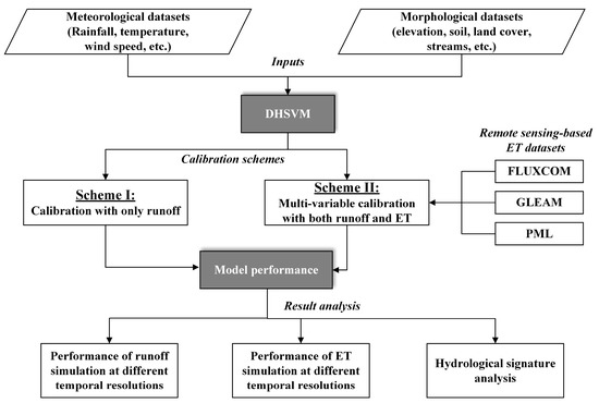
Figure 2.
Flow chart of this study.
4. Results and Discussion
4.1. Evaluation of Remote Sensing-Based ET Datasets
To evaluate the utility of the selected three remote sensing-based ET datasets (namely, PML, FLUXCOM, and GLEAM) in hydrological model performance, the accuracy of these datasets firstly needs to be assessed. In situ observations of pan evaporation are used to evaluate the accuracy of areal ET estimates based on these datasets in 2004–2008, using the five evaluation indices shown in Section 3.3.
As shown in Figure 3, the areal daily remote sensing-based ET estimates are compared with those calculated by in situ observations of pan evaporation from six hydrological stations. Because the temporal resolution of PML is 8 days, the temporal resolution of pan evaporation is redefined to 8 days. Thus, the plot dots in Figure 3 for PML are much fewer than the others. From Figure 3, it can be observed that the areal daily ET from PML, FLUXCOM, and GLEAM is rather consistent with the in situ observations, with high R and KGE values (R > 0.83, and KGE > 0.72), and low PBIAS, RMSE, and ME values (PBIAS < 24.16%, RMSE < 0.86, and abs (ME) < 0.6). This confirms the conclusions found in previous studies, which reveal that the three remote sensing-based ET datasets have high accuracy [26,44,45]. The comparison results reveal that GLEAM has the best performance at the Jinhua River Basin, followed by FLUXCOM and PML. All remote sensing-based ET datasets slightly underestimate the areal daily ET, especially low and high ET values. This is due to the fact that in situ observations of pan evaporation are more similar to PET in humid regions [46]. Figure 4 shows time series of areal monthly ET from the three datasets and in situ observations of pan evaporation. It can be seen that high ET values mainly occur from May to September. As for temporal variation, FLUXCOM and GLEAM present better performance in capturing the dynamics of monthly ET than PML, as PML shows wide underestimation.
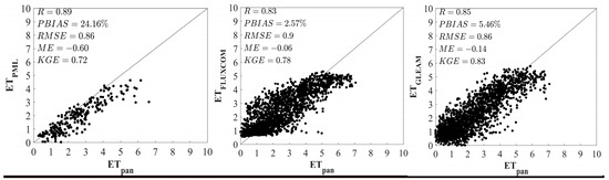
Figure 3.
Comparison of the daily ET data derived from three remote sensing-based datasets with in situ observations of pan evaporation.
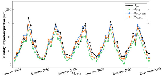
Figure 4.
Temporal comparison of monthly ET between remote sensing-based datasets with in situ observations of pan evaporation.
The differences in the performance of the three remote sensing-based ET datasets are mainly owing to the differences in the forcing data and the algorithms used in the three datasets. As is well known, the three components of ET are vegetation transpiration, soil evaporation, and vaporization of intercepted rainfall. Soil moisture plays a dominant role in soil evaporation. The estimation algorithm of PML lacks the soil moisture as input [28,29]. For FLUXCOM, the index of water availability is calculated for each forcing dataset based on daily precipitation and potential evapotranspiration, which is different from soil moisture [22]. For GLEAM, its separate soil module utilizes precipitation to drive the multi-layer soil model and simultaneously assimilates a remote sensing-based soil moisture dataset, which can increase the accuracy of ET estimates [23,34]. Moreover, because the depth of the soil column affecting the evaporation rate depends on the rooting depth of vegetation, the soil water balance in GLEAM is calculated for each land cover type individually, which is able to improve the ET estimates for different land cover types [26].
4.2. Calibration with Only Runoff (Scheme I)
Scheme I is applied in this section, which only uses the runoff observations for parameter calibration. The KGE and PBIAS of runoff are utilized as objective functions. Besides KGE and PBIAS, the RMSE, R, and ME are used to assess the performance of runoff simulation, which are summarized in Table 2. As shown in Table 2, the KGE values in the calibration and validation periods are 0.87 and 0.89, respectively. The PBIAS values are 3.45% and 4.28% in the calibration and validation periods, respectively. Furthermore, all other evaluation indices are within satisfactory ranges [47]. This illustrates that the model parameters are well calibrated. The good performance of runoff simulation based on Scheme I also can be observed in other studies [7,8].
Table 2.
Evaluation indices of runoff simulation based on Scheme I.
Figure 5 displays the comparison of simulated and observed daily runoff for 2004 and 2009, which is used to represent the calibration and validation periods, respectively. The reason for selecting 2004 and 2009 as the representative years is that the hydrological characteristics of these two years are similar to the calibration and validation periods, respectively. Furthermore, using only one representative year in the figures is beneficial to compare the runoff observations and simulations clearly. As shown in Figure 5, the simulated runoff is very close to the observed runoff in the calibration period, of which almost all peak flows can be captured well. Meanwhile, in the validation period, the value of PBIAS is higher than that in the calibration period, which is mainly due to the underestimation of peak flows. For the peak flows that occurred in June 2009, the model generates a simulated peak flow with 468 m3/s, which is far less than the observation, with 823 m3/s. Furthermore, the observed peak flow is 965 m3/s in August 2009, while the model-simulated peak flow is only 643 m3/s.
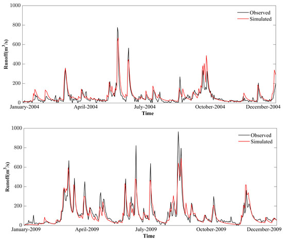
Figure 5.
Comparison of observed and simulated daily runoff in the calibration (2004) and validation periods (2009) based on Scheme I.
Table 3 presents the evaluation indices of ET simulation with the three remote sensing-based ET datasets. From this table, it is obvious that the ET simulation is unsatisfactory. Among these datasets, the simulated ET can replicate the PML-based ET more accurately than the FLUXCOM-based and GLEAM-based ET in the calibration period, with higher KGE and R, and lower PBIAS, RMSE, and ME. However, the performance of ET simulations in the validation period is similar for all three datasets. Overall, it can be concluded that the model based on Scheme I has a better capability to replicate the PML-based ET compared to the FLUXCOM-based and GLEAM-based ET.
Table 3.
Evaluation indices of ET simulation based on Scheme I.
4.3. Multi-Variable Calibration (Scheme II)
4.3.1. Performance Analysis at Different Temporal Resolutions
All three multi-variable calibrations (namely Scheme II (PML), Scheme II (FLUXCOM), and Scheme II (GLEAM)) are applied in this section for parameter calibration. Both the KGE and PBIAS of runoff and ET are utilized as objective functions. To investigate the utility of the three remote sensing-based ET datasets in improving hydrological model simulation (runoff and ET simulations), the hydrological model performance at different temporal resolutions is analyzed.
Regarding the daily temporal resolution, Table 4 presents the evaluation indices of runoff and ET simulations. As shown in Table 4, the performance of runoff simulations based on all three variants of Scheme II is comparable with that based on Scheme I. The KGE values of the runoff simulations based on all three variants of Scheme II are above 0.72 in the calibration period and above 0.85 in the validation period. Furthermore, the value of KGE reaches up to 0.91 in the validation period under Scheme II, and the value is higher than that under Scheme I. In addition, compared to Scheme I, the PBIAS in the validation period for all three Scheme II variants is slightly reduced, but not for the calibration period. A similar situation occurs for ME. The R values under Scheme II are almost the same as that under Scheme I. For RMSE, the values based on Scheme II are slightly increased, but they are still acceptable. For the three ET datasets, the runoff simulation based on Scheme II (PML) has the highest KGE and lowest PBIAS in the calibration period, which are 0.87 and 1.46%, followed by those based on Scheme II (GLEAM) (KGE = 0.75, PBIAS = 9.34%) and Scheme II (FLUXCOM) (KGE = 0.72, PBIAS = 11.82%). Moreover, the RMSE and ME values of the runoff simulation based on Scheme II (PML) are the lowest in the calibration period (RMSE = 74.72, ME = 1.56), followed by those based on Scheme II (GLEAM) (RMSE = 76.10, ME = −9.98) and Scheme II (FLUXCOM) (RMSE = 75.16, ME = −12.62).
Table 4.
Evaluation indices of runoff and ET simulations based on Scheme II.
The relative performance of runoff and ET simulations from all three variants of Scheme II to those from Scheme I are also calculated. The evaluation indices of the ET simulation from Scheme I are based on GLEAM, because of its better accuracy, as stated in Section 4.1. ET simulations from all three variants of Scheme II are greatly improved. The KGE and R values of the ET simulations based on all three variants of Scheme II are increased by up to 45.55% and 35.47% in the calibration period, respectively. The values of PBIAS, RMSE, and ME are decreased by up to 95.85%, 50.97%, and 96.72% in the calibration period, respectively. ET simulations in the validation period show similar performance to those in the calibration period.
Figure 6 shows a temporal comparison of the simulated and observed daily runoff for the calibration (2004) and validation (2009) periods. The figure shows that the DHSVM model calibrated by all three variants of Scheme II can generate reliable runoff simulations. Compared to Scheme I, peak flow simulation based on all three Scheme II variants is greatly improved in the calibration and validation periods. For instance, the observed peak flow is 823 m3/s in June 2009, and the model-generated simulated peak flows are 570 m3/s, 585 m3/s, and 595 m3/s under Scheme II (PML), Scheme II (FLUXCOM), and Scheme II (GLEAM), respectively, while the model under Scheme I generates a simulated peak flow of 468 m3/s. Furthermore, for the peak flow in August 2009, the observation is 965 m3/s; for the model under Scheme I, the simulated peak flow is 643 m3/s, while, for the model under Scheme II, the simulated peak flows are 779 m3/s, 821 m3/s, and 849 m3/s for PML, FLUXCOM, and GLEAM, respectively. The improvement shown in Figure 6 is consistent with the reduction in PBIAS in the validation period presented in Table 4. Overall, the three remote sensing-based ET datasets have the ability to successfully improve the hydrological model simulations at the daily temporal resolution, and PML shows the best improvement in hydrological model performance, followed by GLEAM and FLUXCOM.
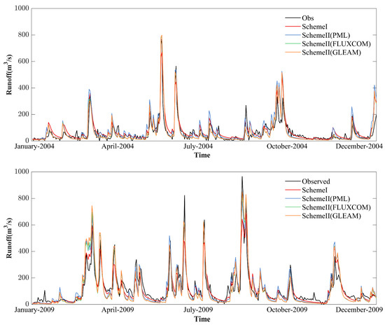
Figure 6.
Comparison of observed and simulated daily runoff in the calibration (2004) and validation periods (2009) based on Scheme I and Scheme II.
Regarding the monthly temporal resolution, KGE and PBIAS values for runoff simulation at different months from all three Scheme II variants are shown in Figure 7. From this figure, it can be observed that the majority of months show good performance, with high KGE and low PBIAS. In terms of KGE, around 58.3%, 58.3%, and 83.3% of months in the calibration period are higher than 0.5 based on Scheme II (FLUXCOM), Scheme II (GLEAM), and Scheme II (PML), respectively. In the validation period, the percentages of months with KGE higher than 0.5 are 83.3% for PML, followed by FLUXCOM (66.7%) and GLEAM (66.7%). As for PBIAS, the percentages of months with PBIAS lower than 25% are 75%, 75%, and 100% for FLUXCOM, GLEAM, and PML in the calibration period, respectively. For the validation period, the percentages are increased to 100%, 91.7%, and 100% for FLUXCOM, GLEAM, and PML, respectively.
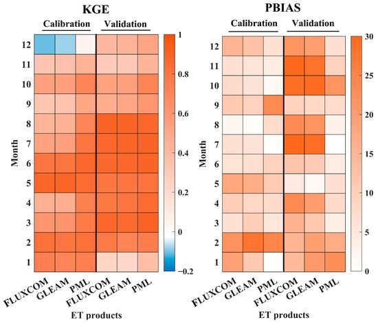
Figure 7.
Comparison of KGE and PBIAS values for runoff simulations in different months based on Scheme II.
Figure 8 shows a temporal comparison of the simulated and observed monthly runoff for the calibration and validation periods based on Scheme I and the three variants of Scheme II. Overall, the DHSVM model calibrated based on Scheme I and all three variants of Scheme II can produce acceptable runoff simulations. Compared to Scheme I, the peak flow simulations based on Scheme II are much closer to the observation than those based on Scheme I in the calibration and validation periods. For example, the observed peak flow is 403 m3/s in June 2008, and the simulated peak flow based on Scheme I is 379 m3/s, while the multi-variable calibrated models generate simulated peak flows of 407 m3/s, 407 m3/s, and 412 m3/s based on Scheme II (PML), Scheme II (FLUXCOM), and Scheme II (GLEAM), respectively. Similar situations can be found in June 2006, March 2010, and July 2010, etc. Moreover, the KGE value is 0.96 in the validation period based on Scheme II (PML), which is higher than that based on Scheme I (KGE = 0.95). The values of PBIAS based on Scheme II are 3.57%, 2.39%, and 0.11% for PML, FLUXCOM, and GLEAM, respectively, which are lower than that based on Scheme I (PBIAS = 4.17%). Among the three datasets, PML slightly outperforms GLEAM and FLUXCOM at the monthly temporal resolution.
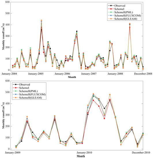
Figure 8.
Comparison of observed and simulated monthly runoff in the calibration and validation periods based on Scheme I and Scheme II.
At the seasonal scale, KGE and PBIAS values for runoff simulations based on Scheme II are compared in Figure 9. In the figure, it is obvious that all three variants of Scheme II present good performance in the four seasons, with high KGE (>0.5) and low PBIAS (<20%). As for KGE, the three ET datasets perform comparably well in spring, summer, and winter, next to autumn, in the calibration and validation periods. Similar conclusions can be derived for PBIAS. Among the three ET datasets, PML performs better than GLEAM and FLUXCOM. The runoff simulation based on Scheme II (PML) has the highest KGE for the four seasons (KGE_Spr = 0.88, KGE_Sum = 0.89, KGE_Aut = 0.77, KGE_Win = 0.81) in the calibration period, followed by Scheme II (GLEAM) (KGE_Spr = 0.75, KGE_Sum = 0.71, KGE_Aut = 0.59, KGE_Win = 0.77) and Scheme II (FLUXCOM) (KGE_Spr = 0.73, KGE_Sum = 0.69, KGE_Aut = 0.58, KGE_Win = 0.78). Similar conclusions can be drawn for the validation period. Furthermore, the runoff simulation under Scheme II (PML) has the lowest value of PBIAS in the calibration period, which is 5.9% for the average value of the four seasons, followed by Scheme II (GLEAM) (14.3%) and Scheme II (FLUXCOM) (14.5%). Meanwhile, the average PBIAS values of the four seasons in the validation period are 7.1%, 5.2%, and 4.6%, respectively.
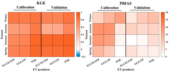
Figure 9.
Comparison of KGE and PBIAS values for runoff simulations at different seasons from Scheme II.
Above all, applying these three ET datasets in model calibration is proven to be capable to improve hydrological model simulations, with enhanced ET simulation and good runoff simulation at different temporal resolutions. The result is consistent with the conclusions obtained in previous studies, which indicate that incorporating ET data into model calibration can maintain runoff simulation and improve ET simulation [7,8]. However, our study reveals more information related to the effect of remote sensing-based ET datasets in improving model performance and the differences among the three ET datasets. The findings in this study can provide a reference for related studies and users under the advancement of remote sensing-based ET datasets. Among the three datasets, PML performs the best in improving model performance, followed by GLEAM and FLUXCOM. The reason for the best performance of PML is because the algorithm used in PML is similar to the ET calculation method adopted in the DHSVM model. The ET calculation in the DHSVM model is based on the Penman–Monteith approach [37]. The method used to estimate ET for the PML dataset is the Penman–Monteith–Leuning energy balance model, which is based on the Penman–Monteith equation, gridded meteorology, and a simple biophysical model for surface conductance (i.e., used with remotely sensed leaf area index to calculate surface conductance) [48,49].
4.3.2. Hydrological Signature Analysis
Hydrological signatures refer to specific characteristics of the hydrograph [50]. The application of hydrological signatures can aid in interpreting the links between models and the underlying hydrological processes, and it provides more information about hydrological model performance [51,52]. Hydrological signatures mainly include rising limb density, peak distribution, runoff ratio, different quantile flows, and flow duration curves (FDCs), etc. Among various hydrological signatures, the FDC is widely used to assess hydrological model performance [21,30]. Therefore, besides regular performance evaluation indices, shown in Section 3.3, the FDC is partitioned into three segments, including low flow (0.7–1.0 flow exceedance probabilities), intermediate flow (0.2–0.7 flow exceedance probabilities), and high flow (0–0.2 flow exceedance probabilities), which are used in this study.
Figure 10 compares the three segments of observed and simulated runoff based on Scheme I and Scheme II. In this figure, it is obvious that the simulated intermediate flow and high flow based on Scheme I and the three variants of Scheme II are much closer to the observation than the low flow. In the calibration period, the simulated low flow and intermediate flow under all calibration schemes tend to be underestimated, and a similar conclusion can be obtained for the validation period. Thus, it is essential to improve the performance of low flow simulations under Scheme I and Scheme II. Compared to Scheme I, the simulated low flow located in the range of exceedance probability 0.97–1.0 (namely, extremely low flows) based on the three variants of Scheme II performs better in the calibration period, and the better performance in the validation period occurs in the range of exceedance probability 0.99–1.0. Furthermore, the simulated intermediate flow located in the range of exceedance probability 0.23–0.26 under Scheme II (PML) is more consistent with the observations in the calibration period. A similar conclusion can be obtained for the validation period when the exceedance probability is within 0.30–0.39. Moreover, the better performance of intermediation flow simulations based on Scheme II (FLUXCOM) and Scheme II (GLEAM) also can be found in the validation period, when the ranges of exceedance probability are 0.22–0.24 and 0.25–0.27 for Scheme II (FLUXCOM) and Scheme II (GLEAM), respectively. The improvement in hydrological model performance based on the three variants of Scheme II is indeed confirmed by their high flow simulations. When the exceedance probability is within 0–0.012—namely, extremely high flows—the runoff simulations based on the three variants of Scheme II outperform that based on Scheme I in the calibration period. In the validation period, a similar improvement can be observed clearly in Figure 10.
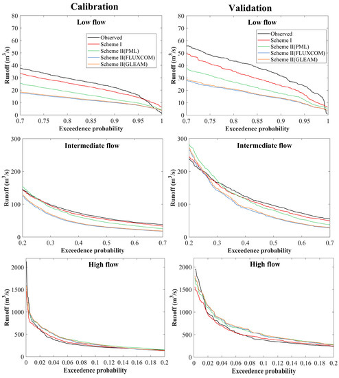
Figure 10.
Comparison of three segments of FDC of observed and simulated daily runoff in the calibration and validation periods based on Scheme I and Scheme II.
Above all, we can conclude that all three variants of Scheme II improve the performance of extreme flow simulations (including extremely low flow and high flow) compared to Scheme I. Low flow and intermediate flow simulations under Scheme II (PML) are more consistent with the observations than those under Scheme II (FLUXCOM) and Scheme II (GLEAM). For high flow, the three variants of Scheme II have comparably good performance in the calibration and validation periods. However, the improvements in extremely high flow simulations based on Scheme II (FLUXCOM) and Scheme II (GLEAM) are almost similar, and it is better than those based on Scheme II (PML). Furthermore, these conclusions are also confirmed by other two hydrological signatures, as presented in Table 5, namely L1 (mean of lowest annual daily flow divided by mean annual daily flow averaged across all years) and H1 (mean of highest annual daily flow divided by mean annual daily flow averaged across all years) [30,53,54]. Based on the result of hydrological signature analysis, PML can be applied to multi-variable calibration in drought forecasting. FLUXCOM and GLEAM are better choices for multi-variable calibration in flood forecasting.
Table 5.
The other two hydrological signatures (L1 and H1) in the calibration and validation periods based on Scheme I and Scheme II.
This study was only conducted in a humid region. Whether similar conclusions can be obtained in other regions, including semi-humid regions, semi-dry regions, and dry regions, is not certain. However, Rajib et al. [21] applied a remote sensing-based ET dataset to multi-variable calibration in a semi-humid region in North Dakota, United States, and the results revealed that the integration of the ET dataset noticeably increased the accuracy in both ET and runoff simulations. Moreover, Becker et al. [2] only used remote sensing-based ET to calibrate model parameters in a semi-humid study area and their results showed that the KGE for individual land use types increased from −0.6 to 0.6. Furthermore, Dembélé et al. [55] applied several multi-variable calibration scenarios with remote sensing-based ET datasets in the Volta River Basin, shared among six countries of West Africa, and the multi-variable calibration scenarios led to higher model performance in all climatic zones of the study area, including humid, semi-humid, semi-arid, and arid zones. In addition, their results demonstrated that the model performance was better in the intermediate climatic regions than in the driest and wettest regions, which is not consistent with Zhang et al. [24]. Zhang et al. [24] used remote sensing-based ET to calibrate two lumped conceptual hydrological models in 222 catchments across Australia and their results revealed that the model performed better in wetter catchments than in drier catchments. Therefore, we can conclude that the integration of remote sensing-based ET datasets into multi-variable calibration is able to improve model performance in semi-humid regions, semi-dry regions, and dry regions, but whether better performance occurs in wetter or in drier regions requires further study. This is subject to many factors, including the selection of hydrological models, study areas, remote sensing-based ET datasets, calibration strategies, etc.
5. Conclusions
This study evaluated the accuracy of three remote sensing-based ET datasets, namely PML, FLUXCOM, and GLEAM, and further investigated the utility of these three datasets in improving the hydrological model performance of DHSVM in the Jinhua River Basin, East China. Firstly, the accuracy of these three ET datasets was assessed against in situ observations of pan evaporation. Afterwards, these ET datasets, together with runoff observations, were utilized for the multi-variable calibration of the DHSVM model. The DHSVM model results calibrated with only runoff were used as a reference. The key findings of this study are summarized below.
- (1)
- All three ET datasets have good performance compared with pan evaporation at the Jinhua River Basin. Among them, FLUXCOM and GLEAM have higher accuracy than PML.
- (2)
- Runoff simulation based on Scheme I shows good performance, with a KGE value of 0.87 in the calibration period and a KGE value of 0.89 in the validation period. The PBIAS values in the calibration and validation period are 3.45% and 4.28%, respectively. However, similar good performance cannot be found in ET simulation.
- (3)
- Scheme II is able to enhance ET simulation and maintain good runoff simulation. Among the three ET datasets, PML performs the best in simulating runoff, with a KGE of 0.87 and a PBIAS of 1.46% in the calibration period and a KEG of 0.91 and a PBIAS of 3.38% in the validation period, and ET simulation is improved with a great reduction in PBIAS (95.85%) and ME (96.72%) in the calibration period. FLUXCOM and GLEAM also show comparable performance in the calibration period.
- (4)
- The DHSVM model calibrated with Scheme II is able to generate reasonable low flow, intermediate flow, and high flow. Compared to Scheme I, Scheme II enhances the performance of extreme flow simulations (including extremely low flow and extremely high flow). PML can be applied to multi-variable calibration in drought forecasting based on the better improvement in extremely low flow simulation. FLUXCOM and GLEAM are good choices for multi-variable calibration in flood forecasting on the basis of the better improvement in extremely high flow simulation.
Author Contributions
Conceptualization, S.P. and Y.-P.X.; Data curation, H.G.; Formal analysis, S.P.; Funding acquisition, S.P.; Investigation, H.G. and W.X.; Methodology, S.P., H.G., B.Y. and W.X.; Project administration, Y.-P.X.; Resources, Y.-P.X.; Software, S.P., H.G., B.Y. and W.X.; Visualization, B.Y.; Writing—original draft, S.P.; Writing—review & editing, Y.-P.X. All authors have read and agreed to the published version of the manuscript.
Funding
This research was funded by the National Nature Science Foundation of China (51909233), the Zhejiang Natural Science Foundation (LY22E090010), and the Key Project of Zhejiang Natural Science Foundation (LZ20E090001).
Data Availability Statement
The meteorological data are provided by the National Climate Center of the China Meteorological Administration and Zhejiang Provincial Metrological Administration. The hydrological data are provided by Zhejiang Provincial Hydrology Administration Center. The ET datasets are provided by GLEAM (https://www.gleam.eu/, accessed on 30 November 2020), PML (https://data.tpdc.ac.cn/zh-hans/data/48c16a8d-d307-4973-abab-972e9449627c/, accessed on 11 December 2020), and FLUXCOM (http://www.fluxcom.org, accessed on 21 December 2020).
Acknowledgments
The valuable comments and suggestions from the editor and three anonymous reviewers are greatly appreciated.
Conflicts of Interest
The authors declare no conflict of interest.
References
- Xie, K.; Liu, P.; Zhang, J.; Wang, G.; Zhang, X.; Zhou, L. Identification of spatially distributed parameters of hydrological models using the dimension-adaptive key grid calibration strategy. J. Hydrol. 2021, 598, 125772. [Google Scholar] [CrossRef]
- Dembélé, M.; Ceperley, N.; Zwart, S.J.; Salvadore, E.; Mariethoz, G.; Schaefli, B. Potential of remote sensing and reanalysis evaporation datasets for hydrological modelling under various model calibration strategies. Adv. Water Resour. 2020, 143, 103667. [Google Scholar] [CrossRef]
- Manfreda, S.; Mita, L.; Dal Sasso, S.F.; Samela, C.; Mancusi, L. Exploiting the use of physical information for the calibration of a lumped hydrological model. Hydrol. Processes 2018, 32, 1420–1433. [Google Scholar] [CrossRef]
- Chlumsky, R.; Mai, J.; Craig, J.R.; Tolson, B.A. Simultaneous calibration of hydrologic model structure and parameters using a blended model. Water Resour. Res. 2021, 57, e2020WR029229. [Google Scholar] [CrossRef]
- Ruiz-Pérez, G.; Koch, J.; Manfreda, S.; Caylor, K.; Francés, F. Calibration of a parsimonious distributed ecohydrological daily model in a data-scarce basin by exclusively using the spatio-temporal variation of NDVI. Hydrol. Earth Syst. Sci. 2017, 21, 6235–6251. [Google Scholar] [CrossRef]
- Gomis-Cebolla, J.; Garcia-Arias, A.; Perpinyà-Vallès, M.; Francés, F. Evaluation of Sentinel-1, SMAP and SMOS surface soil moisture products for distributed eco-hydrological modelling in Mediterranean forest basins. J. Hydrol. 2022, 608, 127569. [Google Scholar] [CrossRef]
- Herman, M.R.; Nejadhashemi, A.P.; Abouali, M.; Hernandez-Suarez, J.S.; Daneshvar, F.; Zhang, Z.; Sharifi, A. Evaluating the role of evapotranspiration remote sensing data in improving hydrological modeling predictability. J. Hydrol. 2018, 556, 39–49. [Google Scholar] [CrossRef]
- Sirisena, T.J.G.; Maskey, S.; Ranasinghe, R. Hydrological model calibration with streamflow and remote sensing based evapotranspiration data in a data poor basin. Remote Sens. 2020, 12, 3768. [Google Scholar] [CrossRef]
- Her, Y.; Seong, C. Responses of hydrological model equifinality, uncertainty, and performance to multi-variable parameter calibration. J. Hydroinform. 2018, 20, 864–885. [Google Scholar] [CrossRef]
- Li, Y.; Grimaldi, S.; Pauwels, V.R.; Walker, J.P. Hydrologic model calibration using remotely sensed soil moisture and discharge measurements: The impact on predictions at gauged and ungauged locations. J. Hydrol. 2018, 557, 897–909. [Google Scholar] [CrossRef]
- Shah, S.; Duan, Z.; Song, X.; Li, R.; Mao, H.; Liu, J.; Wang, M. Evaluating the added value of multi-variable calibration of SWAT with remotely sensed evapotranspiration data for improving hydrological modeling. J. Hydrol. 2021, 603, 127046. [Google Scholar] [CrossRef]
- Ma, D.; Wang, T.; Gao, C.; Pan, S.; Sun, Z.; Xu, Y.P. Potential evapotranspiration changes in Lancang River Basin and Yarlung Zangbo River Basin, southwest China. Hydrol. Sci. J. 2018, 63, 1653–1668. [Google Scholar] [CrossRef]
- Yang, Y.; Chen, R.; Han, C.; Liu, Z. Evaluation of 18 models for calculating potential evapotranspiration in different climatic zones of China. Agric. Water Manag. 2021, 244, 106545. [Google Scholar] [CrossRef]
- Nassar, A.; Torres-Rua, A.; Hipps, L.; Kustas, W.; McKee, M.; Stevens, D.; Coopmans, C. Using remote sensing to estimate scales of spatial heterogeneity to analyze evapotranspiration modeling in a natural ecosystem. Remote Sens. 2022, 14, 372. [Google Scholar] [CrossRef]
- Ruiz-Pérez, G.; González-Sanchis, M.; Del Campo, A.D.; Francés, F. Can a parsimonious model implemented with satellite data be used for modelling the vegetation dynamics and water cycle in water-controlled environments? Ecol. Model. 2016, 324, 45–53. [Google Scholar] [CrossRef]
- Yang, Y.; Anderson, M.; Gao, F.; Xue, J.; Knipper, K.; Hain, C. Improved daily evapotranspiration estimation using remotely sensed data in a data fusion system. Remote Sens. 2022, 14, 1772. [Google Scholar] [CrossRef]
- Melo, D.C.D.; Anache, J.A.A.; Borges, V.P.; Miralles, D.G.; Martens, B.; Fisher, J.B.; Wendland, E. Are remote sensing evapotranspiration models reliable across South American ecoregions? Water Resour. Res. 2021, 57, e2020WR028752. [Google Scholar] [CrossRef]
- Wu, J.; Lakshmi, V.; Wang, D.; Lin, P.; Pan, M.; Cai, X.; Zeng, Z. The reliability of global remote sensing evapotranspiration datasets over Amazon. Remote Sens. 2020, 12, 2211. [Google Scholar] [CrossRef]
- Paca, V.H.D.M.; Espinoza-Dávalos, G.E.; Hessels, T.M.; Moreira, D.M.; Comair, G.F.; Bastiaanssen, W.G. The spatial variability of actual evapotranspiration across the Amazon River Basin based on remote sensing datasets validated with flux towers. Ecol. Processes 2019, 8, 6. [Google Scholar] [CrossRef]
- Poméon, T.; Diekkrüger, B.; Kumar, R. Computationally efficient multivariate calibration and validation of a grid-based hydrologic model in sparsely gauged West African river basins. Water 2018, 10, 1418. [Google Scholar] [CrossRef] [Green Version]
- Rajib, A.; Evenson, G.R.; Golden, H.E.; Lane, C.R. Hydrologic model predictability improves with spatially explicit calibration using remotely sensed evapotranspiration and biophysical parameters. J. Hydrol. 2018, 567, 668–683. [Google Scholar] [CrossRef] [PubMed]
- Jung, M.; Koirala, S.; Weber, U.; Ichii, K.; Gans, F.; Camps-Valls, G.; Reichstein, M. The FLUXCOM ensemble of global land-atmosphere energy fluxes. Sci. Data 2019, 6, 74. [Google Scholar] [CrossRef] [PubMed]
- Martens, B.; Miralles, D.G.; Lievens, H.; Van Der Schalie, R.; De Jeu, R.A.; Fernández-Prieto, D.; Verhoest, N.E. GLEAM v3: Remote sensing-based land evaporation and root-zone soil moisture. Geosci. Model Dev. 2017, 10, 1903–1925. [Google Scholar] [CrossRef]
- Zhang, Y.; Chiew, F.H.; Liu, C.; Tang, Q.; Xia, J.; Tian, J.; Li, C. Can remotely sensed actual evapotranspiration facilitate hydrological prediction in ungauged regions without runoff calibration? Water Resour. Res. 2020, 56, e2019WR026236. [Google Scholar] [CrossRef]
- Tramontana, G.; Jung, M.; Schwalm, C.R.; Ichii, K.; Camps-Valls, G.; Ráduly, B.; Papale, D. Predicting carbon dioxide and energy fluxes across global FLUXNET sites with regression algorithms. Biogeosciences 2016, 13, 4291–4313. [Google Scholar] [CrossRef]
- Yang, X.; Yong, B.; Ren, L.; Zhang, Y.; Long, D. Multi-scale validation of GLEAM evapotranspiration datasets over China via ChinaFLUX ET measurements. Int. J. Remote Sens. 2017, 38, 5688–5709. [Google Scholar] [CrossRef]
- Zhang, Y.; Peña-Arancibia, J.L.; McVicar, T.R.; Chiew, F.H.S.; Vaze, J.; Liu, C.; Lu, X.; Zheng, H.; Wang, Y.; Liu, Y.Y.; et al. Multi-decadal trends in global terrestrial evapotranspiration and its components. Sci. Rep. 2016, 6, 19124. [Google Scholar] [CrossRef]
- Zhang, Y.; Kong, D.; Gan, R.; Chiew, F.H.S.; McVicar, T.R.; Zhang, Q.; Yang, Y. Coupled estimation of 500m and 8-day resolution global evapotranspiration and gross primary datasetion in 2002-2017. Remote Sens. Environ. 2019, 222, 165–182. [Google Scholar] [CrossRef]
- Zhang, Y. PML_V2 Global Evapotranspiration and Gross Primary Datasetion (2002.07–2019.08); National Tibetan Plateau Data Center: Beijing, China, 2020. [Google Scholar]
- Pan, S.; Fu, G.; Chiang, Y.M.; Ran, Q.; Xu, Y.P. A two-step sensitivity analysis for hydrological signatures in Jinhua River Basin, East China. Hydrol. Sci. J. 2017, 62, 2511–2530. [Google Scholar] [CrossRef]
- Xu, Y.P.; Gao, X.; Zhu, Q.; Zhang, Y.; Kang, L. Coupling a regional climate model and a distributed hydrological model to assess future water resources in Jinhua River Basin, East China. J. Hydrol. Eng. 2015, 20, 04014054. [Google Scholar] [CrossRef]
- FLUXCOM. FLUXCOM Global Energy and Carbon Fluxes; Max Planck Institute for Biogeochemistry: Jena, Germany, 2017. [Google Scholar]
- Jung, M.; Reichstein, M.; Schwalm, C.R.; Huntingford, C.; Sitch, S.; Ahlström, A.; Zeng, N. Compensatory water effects link yearly global land CO2 sink changes to temperature. Nature 2017, 541, 516–520. [Google Scholar] [CrossRef] [PubMed]
- Miralles, D.G.; De Jeu, R.A.M.; Gash, J.H.; Holmes, T.R.H.; Dolman, A.J. Magnitude and variability of land evaporation and its components at the global scale. Hydrol. Earth Syst. Sci. 2011, 15, 967–981. [Google Scholar] [CrossRef]
- Wigmosta, M.S.; Vail, L.W.; Lettenmaier, D.P. A distributed hydrology-vegetation model for complex terrain. Water Resour. Res. 1994, 30, 1665–1679. [Google Scholar] [CrossRef]
- Wigmosta, M.S.; Burges, S.J. An adaptive modeling and monitoring approach to describe the hydrologic behavior of small catchments. J. Hydrol. 1997, 202, 48–77. [Google Scholar] [CrossRef]
- Wigmosta, M.S.; Nijssen, B.; Storck, P.; Lettenmaier, D.P. The Distributed Hydrology Soil Vegetation Model; Mathematical Models of Small Watershed Hydrology and Applications; US Department of Energy: Oak Ridge, TN, USA, 2002; pp. 7–42. [Google Scholar]
- Cuo, L.; Giambelluca, T.W.; Ziegler, A.D. Lumped parameter sensitivity analysis of a distributed hydrological model within tropical and temperate catchments. Hydrol. Processes 2011, 25, 2405–2421. [Google Scholar] [CrossRef]
- Xu, Y.P.; Pan, S.; Fu, G.; Tian, Y.; Zhang, X. Future potential evapotranspiration changes and contribution analysis in Zhejiang Province, East China. J. Geophys. Res.: Atmos. 2014, 119, 2174–2192. [Google Scholar] [CrossRef]
- Sun, N.; Yearsley, J.; Voisin, N.; Lettenmaier, D.P. A spatially distributed model for the assessment of land use impacts on stream temperature in small urban watersheds. Hydrol. Processes 2015, 29, 2331–2345. [Google Scholar] [CrossRef]
- Pan, S.; Liu, L.; Bai, Z.; Xu, Y.P. Integration of remote sensing evapotranspiration into multi-variable calibration of distributed hydrology–soil–vegetation model (DHSVM) in a humid region of China. Water 2018, 10, 1841. [Google Scholar] [CrossRef]
- Gupta, H.V.; Kling, H.; Yilmaz, K.K.; Martinez, G.F. Decomposition of the mean squared error and NSE performance criteria: Implications for improving hydrological modelling. J. Hydrol. 2009, 377, 80–91. [Google Scholar] [CrossRef]
- Kling, H.; Fuchs, M.; Paulin, M. Runoff conditions in the upper Danube basin under an ensemble of climate change scenarios. J. Hydrol. 2012, 424, 264–277. [Google Scholar] [CrossRef]
- Li, C.; Zhang, Y.; Shen, Y.; Kong, D.; Zhou, X. LUCC-driven changes in gross primary datasetion and actual evapotranspiration in northern China. J. Geophys. Res. Atmos. 2020, 125, e2019JD031705. [Google Scholar]
- Ma, N.; Szilagyi, J.; Jozsa, J. Benchmarking large-scale evapotranspiration estimates: A perspective from a calibration-free complementary relationship approach and FLUXCOM. J. Hydrol. 2020, 590, 125221. [Google Scholar] [CrossRef]
- Althoff, D.; Rodrigues, L.N.; da Silva, D.D.; Bazame, H.C. Improving methods for estimating small reservoir evaporation in the Brazilian Savanna. Agric. Water Manag. 2019, 216, 105–112. [Google Scholar] [CrossRef]
- Safeeq, M.; Fares, A. Hydrologic response of a Hawaiian watershed to future climate change scenarios. Hydrol. Processes 2012, 26, 2745–2764. [Google Scholar] [CrossRef]
- Leuning, R.; Zhang, Y.Q.; Rajaud, A.; Cleugh, H.; Tu, K. A simple surface conductance model to estimate regional evaporation using MODIS leaf area index and the Penman-Monteith equation. Water Resour. Res. 2008, 44, 10. [Google Scholar] [CrossRef]
- Zhang, Y.; Leuning, R.; Hutley, L.B.; Beringer, J.; McHugh, I.; Walker, J.P. Using long-term water balances to parameterize surface conductances and calculate evaporation at 0.05 spatial resolution. Water Resour. Res. 2010, 46, 5. [Google Scholar] [CrossRef]
- Euser, T.; Winsemius, H.C.; Hrachowitz, M.; Fenicia, F.; Uhlenbrook, S.; Savenije, H.H.G. A framework to assess the realism of model structures using hydrological signatures. Hydrol. Earth Syst. Sci. 2013, 17, 1893–1912. [Google Scholar] [CrossRef]
- Addor, N.; Nearing, G.; Prieto, C.; Newman, A.J.; Le Vine, N.; Clark, M.P. A ranking of hydrological signatures based on their predictability in space. Water Resour. Res. 2018, 54, 8792–8812. [Google Scholar] [CrossRef]
- McMillan, H.; Westerberg, I.; Branger, F. Five guidelines for selecting hydrological signatures. Hydrol. Processes 2017, 31, 4757–4761. [Google Scholar] [CrossRef]
- Olden, J.D.; Poff, N.L. Redundancy and the choice of hydrologic indices for characterizing streamflow regimes. River Res. Appl. 2003, 19, 101–121. [Google Scholar] [CrossRef]
- Oudin, L.; Hervieu, F.; Michel, C.; Perrin, C.; Andréassian, V.; Anctil, F.; Loumagne, C. Which potential evapotranspiration input for a lumped rainfall–runoff model?: Part 2—Towards a simple and efficient potential evapotranspiration model for rainfall–runoff modelling. J. Hydrol. 2005, 303, 290–306. [Google Scholar] [CrossRef]
- Becker, R.; Koppa, A.; Schulz, S.; Usman, M.; aus der Beek, T.; Schueth, C. Spatially distributed model calibration of a highly managed hydrological system using remote sensing-derived ET data. J. Hydrol. 2019, 577, 123944. [Google Scholar] [CrossRef]
Publisher’s Note: MDPI stays neutral with regard to jurisdictional claims in published maps and institutional affiliations. |
© 2022 by the authors. Licensee MDPI, Basel, Switzerland. This article is an open access article distributed under the terms and conditions of the Creative Commons Attribution (CC BY) license (https://creativecommons.org/licenses/by/4.0/).