Article

Deep Learning to Near-Surface Humidity Retrieval from Multi-Sensor Remote Sensing Data over the China Seas

1
State Key Laboratory of Tropical Oceanography, South China Sea Institute of Oceanology, Chinese Academy of Sciences, Guangzhou 510301, China
2
Southern Marine Science and Engineering Guangdong Laboratory (Guangzhou), Guangzhou 511458, China
3
Innovation Academy of South China Sea Ecology and Environmental Engineering, Chinese Academy of Sciences, Guangzhou 511458, China
4
University of Chinese Academy of Sciences, Beijing 100049, China
*
Author to whom correspondence should be addressed.
Remote Sens. 2022, 14(17), 4353; https://doi.org/10.3390/rs14174353
Submission received: 4 July 2022 / Revised: 24 August 2022 / Accepted: 26 August 2022 / Published: 2 September 2022
(This article belongs to the Special Issue AI for Marine, Ocean and Climate Change Monitoring)

Abstract

:
Near-surface humidity (Qa) is a key parameter that modulates oceanic evaporation and influences the global water cycle. Remote sensing observations act as feasible sources for long-term and large-scale Qa monitoring. However, existing satellite Qa retrieval models are subject to apparent uncertainties due to model errors and insufficient training data. Based on in situ observations collected over the China Seas over the last two decades, a deep learning approach named Ensemble Mean of Target deep neural networks (EMTnet) is proposed to improve the satellite Qa retrieval over the China Seas for the first time. The EMTnet model outperforms five representative existing models by nearly eliminating the mean bias and significantly reducing the root-mean-square error in satellite Qa retrieval. According to its target deep neural network selection process, the EMTnet model can obtain more objective learning results when the observational data are divergent. The EMTnet model was subsequently applied to produce 30-year monthly gridded Qa data over the China Seas. It indicates that the climbing rate of Qa over the China Seas under the background of global warming is probably underestimated by current products.

Graphical Abstract

1. Introduction

As the primary source of global evaporation and precipitation, the ocean plays an important role in the transportation and redistribution of water resources on Earth [1,2,3]. On this basis, the near-surface humidity (Qa) over global oceans is crucial, as it modulates oceanic evaporation and influences the global water cycle [4,5,6]. Nevertheless, there are non-negligible uncertainties in Qa estimates in satellite-derived products [7,8] and reanalysis products [9,10]. The imperfection of Qa data quality has been reported as one of the leading error sources of uncertainties in freshwater exchanges across the air–sea interface and in global water budgets [11,12,13,14]. Even in coupled general circulation models, the performance of Qa is highly related to simulations of oceanic evaporation [15]. Accurate estimates of Qa are thus necessary for studies on the global water cycle, air–sea interactions, and climate change [16].
The measurements of Qa can be generally divided into two approaches: in situ observations and remote sensing observations. The former are direct measurements of Qa and have relatively high credibility, but these observations are subject to poor continuity in time and space. The latter have the advantage of long-term and large-scale Qa monitoring. Still, remote sensing is an indirect approach that requires a relevant retrieval model to convert satellite measurements into Qa. With the development of space-borne technology and microwave radiometers, the last several decades have experienced the prosperity of investigations in model development for satellite Qa retrieval. Considering that a large portion of the total column precipitable water (TPW) is confined in the atmospheric surface layer, pioneering work by [17,18] (hereafter L86) linked the TPW to Qa in light of the QaW relation. It was reported that the QaW relationship has excellent performance with training data on a monthly scale [18] and can also work well with synoptic-scale data [19]. Considering the decoupling of the atmospheric boundary layer from the upper troposphere, Ref. [20] proposed replacing the TPW data in the QaW relation with the precipitable water constrained in the lowest 500 m, which can be derived from brightness temperature (TB) measurements. To reduce the propagation of uncertainties within input data, Ref. [21] established a direct linear regression between Qa and TB. Under the scheme of the QaW relation, Ref. [22] developed an empirical orthogonal function method for satellite Qa retrieval. A neural network combining TPW and sea surface temperature (SST) was first developed to estimate Qa by [23]. Subsequently, estimates of Qa with multichannel TBs as input data by multivariate linear regression [24,25,26,27] or nonlinear regression [16,28,29] prevailed in the last two decades.
The models above were primarily designed for global oceans. However, Ref. [28] reported that satellite Qa retrieval differed in regions of the tropics and high latitudes, and a high-latitude enhancement was considered in their model. It indicates that attention should be given to different regional features of satellite Qa retrieval. The China Seas, consisting of the Bohai Sea, Yellow Sea (YS), East China Sea (ECS), and South China Sea (SCS), are the largest marginal group of seas in the northwestern Pacific and are strongly influenced by complex continental environments. Previous investigations have pointed out that the Qa data in this region suffer from significant uncertainties and are the leading error source of air–sea heat fluxes [30,31].
In recent years, machine learning, especially deep learning, has been widely used to provide new insights into traditional and/or emerging research in earth science [32,33,34,35,36]. With the accumulation of high-quality in situ observations of Qa over the China Seas in the last two decades, the main objective of this study is to develop a deep-learning-based model to improve the satellite Qa retrieval over the China Seas. The data and methods are introduced in Section 2. The main results are presented in Section 3. Section 4 discusses the interpretability of the deep-learning-based model. Finally, Section 5 draws the main conclusion of this study.

2. Data and Methods

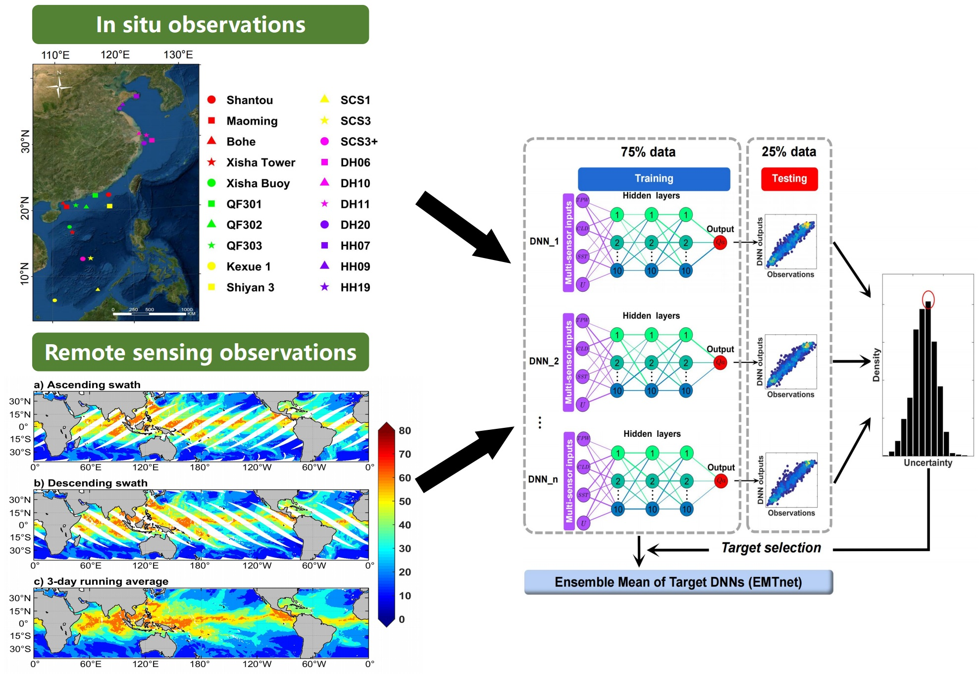
2.1. In Situ Observations

In situ observation information from this study is listed in Table 1. There are 20 observational stations in the coastal and open oceans (Figure 1a), including 18 buoys, 1 offshore platform, and 1 flux tower on an island. Compared to ship observations, these fixed-point observations usually have more stable data quality performance. The data collected in coastal areas are valuable touchstones to validate the performance of remote sensing observations, including Qa, surface wind, and sea surface temperature. The data span from 1998 to 2018, and the sampling intervals vary from 1 min to 30 min. All the raw data were processed with quality control procedures as suggested by [31,37,38]. For all stations, the Qa and surface wind data were adjusted to standard heights of 2 m and 10 m, respectively, according to the COARE 3.0 algorithm [39].
The basic characteristics of in situ observations of Qa are examined to check their representativeness, considering many missing data and the uneven sampling in time and space. As shown in Figure 1b–d, Qa varies from 5.5 to 24.0, 1.5 to 24.5, and 0.8 to 24.8 g/kg in the SCS, ECS, and YS. Qa’s mean values plus/minus one standard deviation (STD) are 16.6 ± 4.1, 10.1 ± 5.5, and 8.5 ± 5.7 g/kg in the SCS, ECS, and YS. For the probability density distributions (PDDs) of Qa, a left-skewed distribution in the SCS and right-skewed distributions in the ECS and YS can be observed. These lower limits, mean values, and PDDs of Qa in the three seas coincide well with the latitudes they locate in, as Qa usually decreases from low to high latitudes. With the data in the three seas considered as a whole, Qa presents a fairly even distribution in the range of 2~22 g/kg, which varies basically around a steady density across each bin (Figure 1e). The highly uniform PDD of Qa shows an acceptable representativeness of in situ observations collected here. Therefore, it is expected that the analyses based on those data could be relatively objective and with high significance.

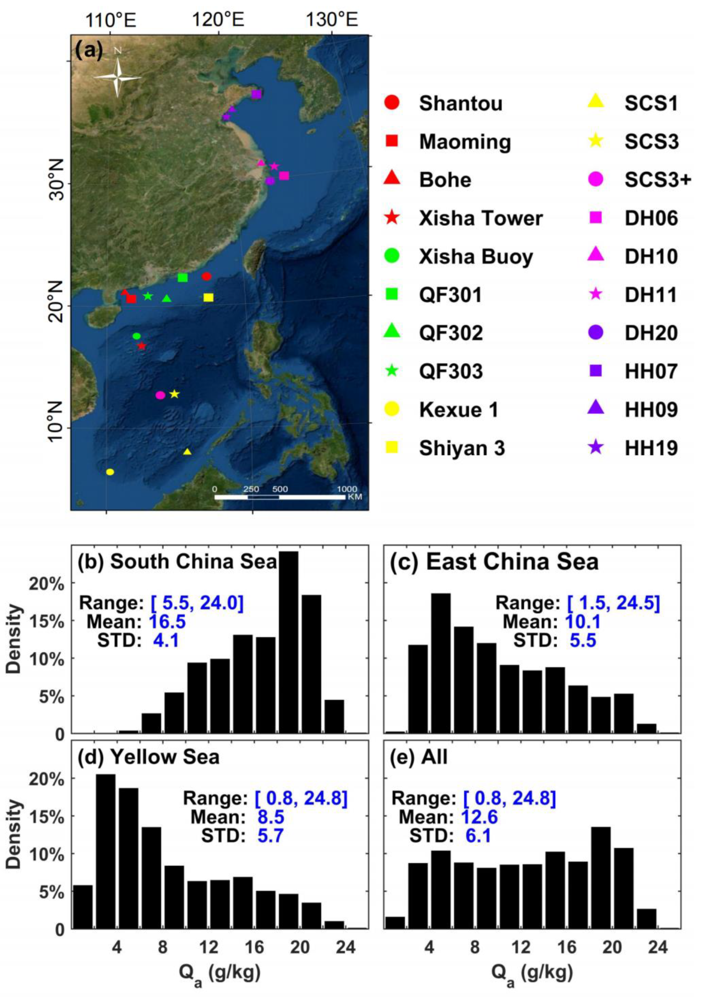
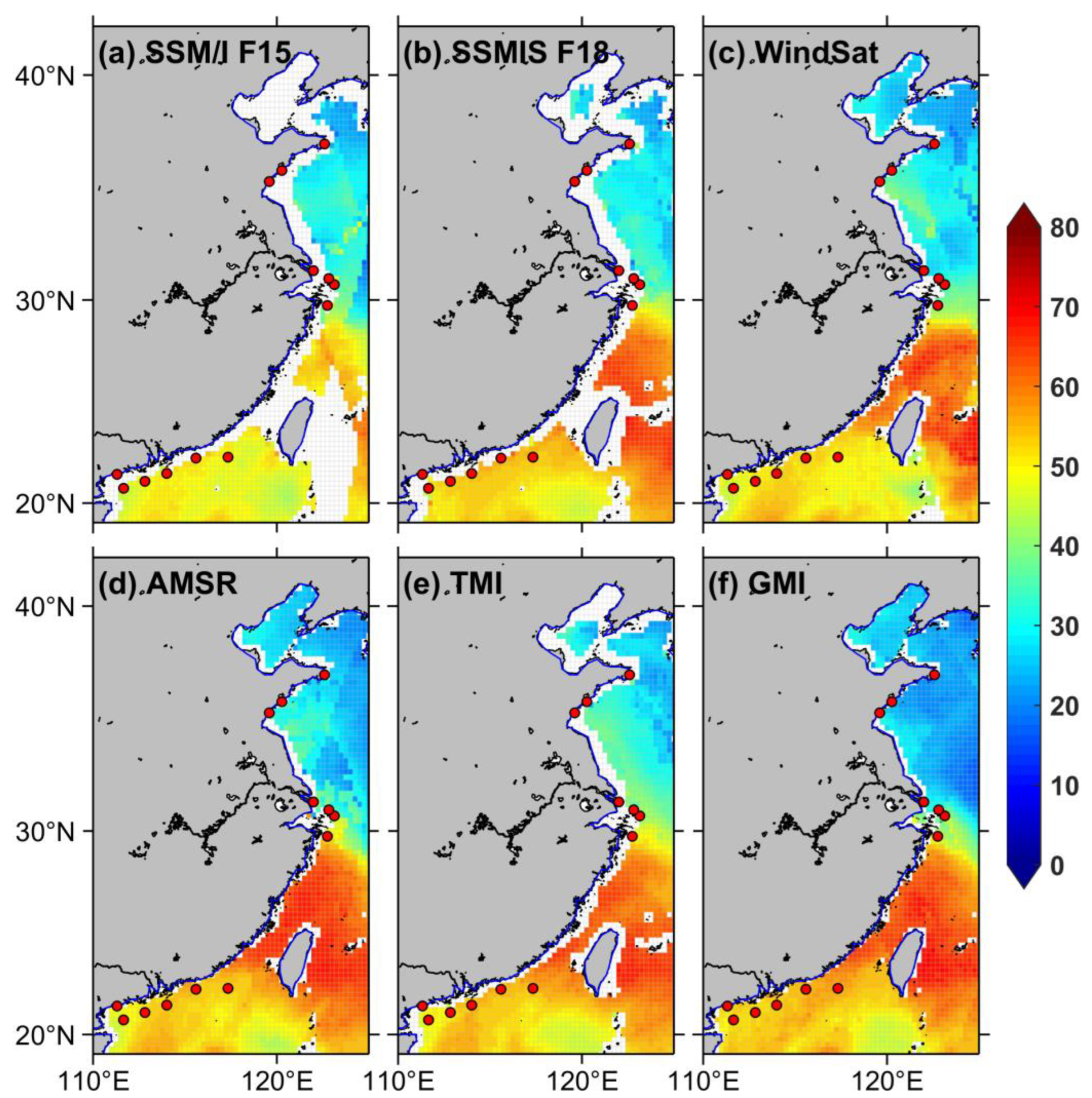
2.2. Remote Sensing Data

Remote sensing observations of TPW, wind speed (U), cloud liquid water (CLW), and SST from various satellite microwave radiometers are utilized in this study. The sensors include the Special Sensor Microwave Imager (SSM/I), the Special Sensor Microwave Imager Sounder (SSMIS), the Advanced Microwave Scanning Radiometer series (AMSR-E and AMSR-2), the WindSat Polarimetric Radiometer, the Tropical Rainfall Measuring Mission (TRMM) Microwave Imager (TMI), and the Global Precipitation Measurement Microwave Imager (GMI). For SSM/I and SSMIS, the instruments are referred to by satellite number starting with F08. Here, F15 from SSMI/I and F16 to F18 from SSMIS are employed because of their relatively long time coverage. Detailed descriptions for each sensor can be found at the Remote Sensing Systems (RSS; www.remss.com, accessed on 30 June 2022). Due to the satellite swath width and orbit seam, banded gaps exist in the ascending and descending daily maps of satellited-derived variables. To facilitate the matching of satellite data and in situ data, the products incorporating both the ascending and descending data by using 3-day running average are utilized, which can achieve more homogeneous spatial distributions for these variables. Note that there exist differences in data from various sensors (Figure 2), and uncertainties in results may be caused by a single data source. Consequently, multi-sensor inputs from SSM/I F15, SSMIS F16, SSMIS F17, SSMIS F18, AMSR-E, AMSR-2, WindSat, TMI, and GMI are utilized in the following study.
TB data from six channels are used for the models listed in Table 2 that directly retrieve Qa from multichannel TBs. These channels are 19 H, 19 V, 22 V, and 37 V GHz from SSMIS F17 and 52 V GHz from Advanced Microwave Sounding Unit-A (AMSU-A), where H and V denote the horizontal and vertical polarizations, respectively. As underscored by RSS, TBs from the SSMIS are produced using uniform processing techniques. They are intercalibrated by considering the differences in sensor frequencies, channel resolutions, instrument operation, and other radiometer characteristics [40]. The AMSU-A is a multichannel microwave radiometer that performs atmospheric sounding of temperature and moisture by passively recording atmospheric microwave radiation at multiple wavelengths. Detailed descriptions of how TBs from the AMSU-A are processed can be found in [41,42]. The collocating strategy between satellite data and in situ observations for each station is as follows:
(i) For variables TPW, U, and CLW, which are already in daily values, first, average the high-frequency in situ observations to daily values with the local standard time adjusted to Coordinated Universal Time and then apply a 3-day running average. Second, locate the 0.25° × 0.25° box in the satellite data where the corresponding observational station lies. Subsequently, the mean value of the four corners of that box is used as a proxy for satellite data. Attempts such as extending the search area to 1° × 1° box and/or applying an inverse-distance-weighted average present similar results.
(ii) For TBs with ascending and descending measurements per day, temporal and spatial windows of 90 min and 50 km following Yu and Jin (2018) are used. If multiple points of satellite data meet the criterion, the average of those points is taken. If no satellite data match the in situ observations, a missing value is set.
Table 2. Summary of the methods of surface humidity retrieval validated in this study. Here, the W denotes the parameter TPW in the main text.
AlgorithmEquationRMSE (g/kg)
Liu et al. (1986) [18] Q a = C 1 × W + C 2 × W 2 + C 3 × W 3 + C 4 × W 4 + C 5 × W 5 ,
where C1 = 0.006088244, C2 = 0.1897219, C3 = 0.1891893, C4 = −0.07549036, and C5 = 0.006088244.
0.40 in tropics and 0.80 in globe
Jones et al. (1999) [23] Q a = C 0 + C 1 × S S T + C 2 × S S T 2 + C 3 × W 1 + C 4 × W 2 ,
where C0 = 2.1052, C1 = −0.0551, C2 = 0.0138, C3 = 0.2435, and C4 = −0.0019.
0.77 ± 0.39
Bentamy et al. (2003) [24] Q a = C 0 + C 1 T 19 V + C 2 T 19 H + C 3 T 22 V + C 4 T 37 V , where C0 = −55.9227, C1 = 0.4035, C2 = −0.2944, C3 = 0.3511, and C4 = −0.2395.1.40
Jackson et al. (2006) [25] Q a = C 0 + C 1 T 52 V + C 2 T 19 V + C 3 T 19 H + C 4 T 37 V , where C0 = −105.117, C1 = 0.31743, C2 = 0.62754, C3 = −0.12056, and C4 = −0.33940.0.83
Yu and Jin (2018) [28] Q a = a 0 + a 1 T 19 v + a 2 T 22 v + a 3 T 37 v + a 4 T 52 v + b 1 T 19 v 2 + b 2 T 22 v 2 + b 3 T 37 v 2 + b 4 T 52 v 2 , where a0 = 1423.34, a1 = 0.46967, a2 = 0.43401, a3 = −0.92292, a4 = −11.494, b1 = −0.00071, b2 = −0.00072, b3 = 0.00155, and b4 = 0.02336 for the global model, a0 = −127.10, a1 = −0.21113, a2 = 0.71712, a3 = −0.78268, a4 = 1.1918, b1 = 0.00062, b2 = −0.00139, b3 = 0.00153, and b4 = −0.00222 for the high-latitude model.0.82

2.3. Reanalysis Data

Two reanalysis products are employed to make comparisons with the Qa data derived from the model proposed in this study. They are the European Centre for Medium Range Weather Forecast (ECWMF) fifth generation (ERA5) reanalysis product [43] and the National Centers for Environmental Prediction/Department of Energy Global Reanalysis 2 (NCEP2) product [44]. Both products are the latest versions of their corresponding series and improvements have been made in their data assimilations and model physics. Monthly Qa data from 1990 to 2019 are extracted from the two reanalyses and are interpolated onto 1° × 1° grid maps.

2.4. Existing Satellite Qa Retrieval Models

Five representative satellite Qa retrieval models are employed to intercompare with the deep-learning-based model proposed in this study. Table 2 summarizes the basic information of these five models. The L86 model uses a fifth-order polynomial regression approach to estimate Qa with TPW data. The model reported in [23] (hereafter J99) uses a nonlinear neural network approach to estimate Qa with TPW and SST. The models reported in [24] (hereafter B03) and [25] (hereafter J06) use multivariate linear regression to estimate Qa with multichannel TBs. Recently, the model reported in [28] (hereafter Y18) uses multivariate nonlinear regression to estimate Qa with multichannel TBs and considers enhancement in high latitudes.

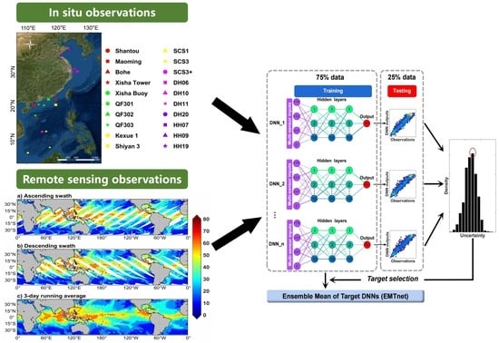
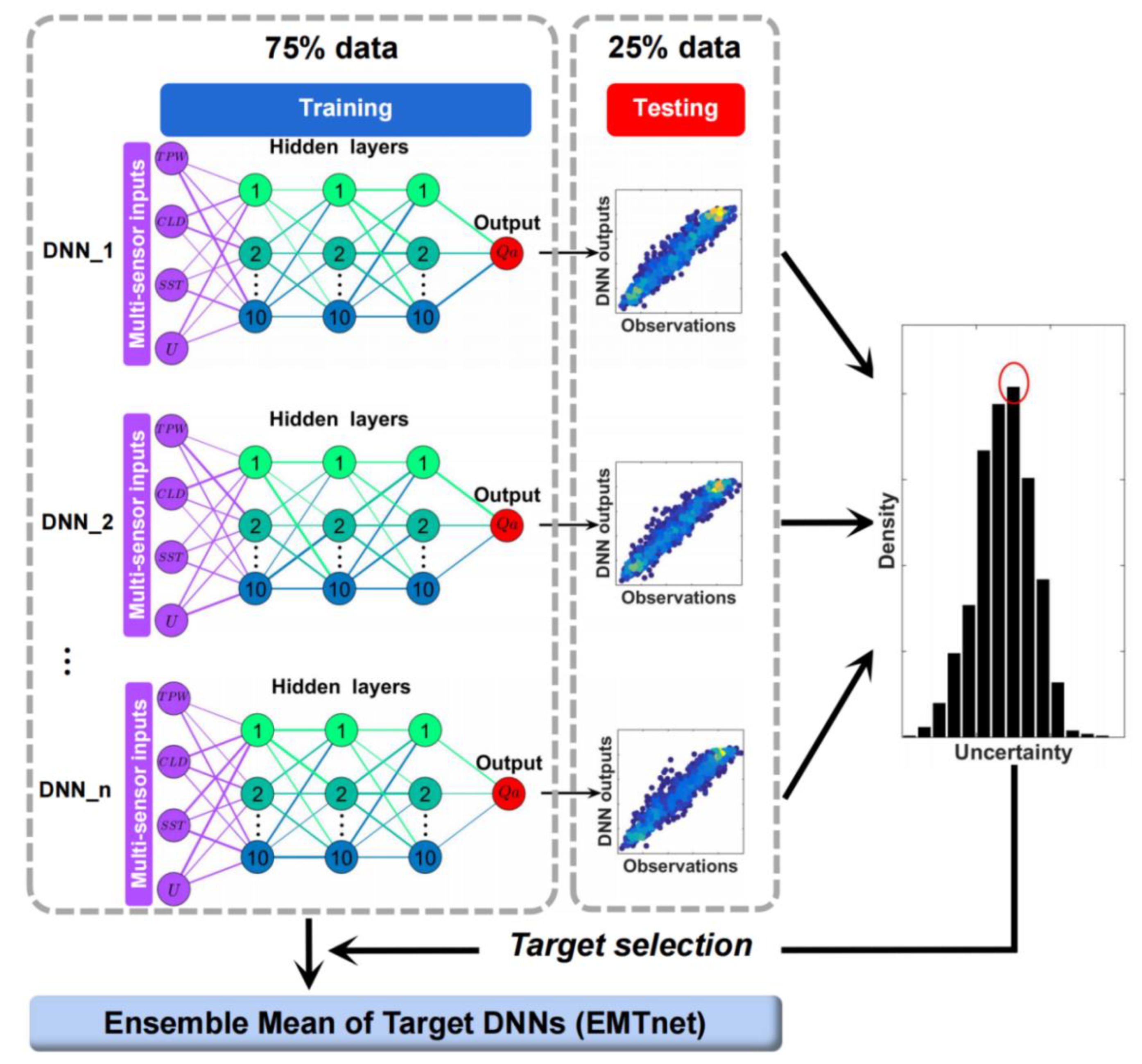
2.5. Ensemble Mean of Target Deep Neural Network Development

A model named Ensemble Mean of Target deep neural networks (EMTnet) was proposed to improve the satellite Qa retrieval over the China Seas (Figure 3). The tool to build and perform the EMTnet model is TensorFlow (https://tensorflow.org/, accessed on 30 June 2022), an open-source machine learning library. The EMTnet model is generated from a large number of deep neural networks (DNNs). Each DNN is based on the error backpropagation (BP) algorithm [45] and consists of an input layer, three hidden layers, and an output layer. The BP algorithm takes advantage of the gradient descent and error backpropagation methods to adjust the connection weights of corresponding neurons to achieve its nonlinear learning ability. The EMTnet model works via the following steps:
(i) Four satellite-derived variables, TPW, CLW, U, and SST, are put in the input layer of each DNN. Note that different combinations of input variables can lead to different learning abilities of the EMTnet model, which are discussed in Section 4. Attempts using pure multichannel TBs or the mix of level-3 variables and multichannel TBs show similar or even slightly worse results.
(ii) Normalize these four input variables to the range between 0 and 1 according to their maximum and minimum values. It is known that the DNNs are quite sensitive to the magnitude difference in various input variables. Therefore, normalizing the input variables in advance can lead to better computational efficiency and results.
(iii) Determine the specific configuration of each DNN. The EMTnet model does not necessarily use the DNN approach. We have also tried other machine learning approaches such as the support vector machine (SVM) and the random forest (RF). It is found that the results of SVM and RF were comparable with those of the DNN, or sometimes slightly worse. The DNN approach is eventually employed to build the EMTnet model considering its better abilities in big data processing efficiency and nonlinear learning ability. Critical parameters are eventually determined through a number of tests to make the DNNs suitable for the learning task here. For instance, three hidden layers, each with ten neurons, are used. The number of iterations is set to 5000, and the learning rate is set to 0.005. In addition, the activation function is essential in forming nonlinear learning abilities for the DNNs. Three widely used activation functions, sigmoid, rectified linear units (ReLU), and hyperbolic tangent function (tanh), have been tested and compared. These activation functions have some defects, for example, the neuronal death for the ReLU activation function and a vanishing gradient for the sigmoid activation function. Activation function tanh is free of neuronal death, and the vanishing gradient problem has been alleviated to some extent. In addition, tanh has a faster convergence speed and a lower number of iterations. Preliminary tests show that the sigmoid and tanh activation functions perform better than the ReLU activation function in this study. Further inspections find that the accuracy of the result using the tanh activation function is 2~4% higher than that using the sigmoid activation function. Therefore, the tanh activation function is employed in this study. Note the current hyper-parameter tuning for each DNN is not unique. It only aims to make each DNN suitable for the learning task here. For those who are interested in the EMTnet model, they can adjust these hyper-parameter tunings according to specific tasks.
(iv) A total of 75% of Qa observations are randomly sampled as training data, while the remaining 25% are used as independent testing data. As for traditional DNN training and testing, this operation is usually conducted once. However, it is found that samplings of different training and testing data can result in different uncertainty levels for the DNNs. To reduce the uncertainty of learning results caused by man-made operations in setting training and testing data, the Ensemble Mean approach is adopted. The EMTnet model trains n different DNNs with randomly sampled n sets of training and testing data to produce an ensemble of DNNs. In this study, the n is set to 1000. For each DNN, the testing data are used to compute the mean bias and root-mean-square error (RMSE). The sum of absolute values of mean bias and RMSE, that is, the absolute error, is taken as the uncertainty of each DNN.
According to the PDD of uncertainties constructed by the DNN ensemble, the top 10% DNNs with uncertainties falling into the highest density intervals are selected as target DNNs. The Ensemble Mean of Target DNNs is then used to produce the EMTnet model outputs.

3. Results

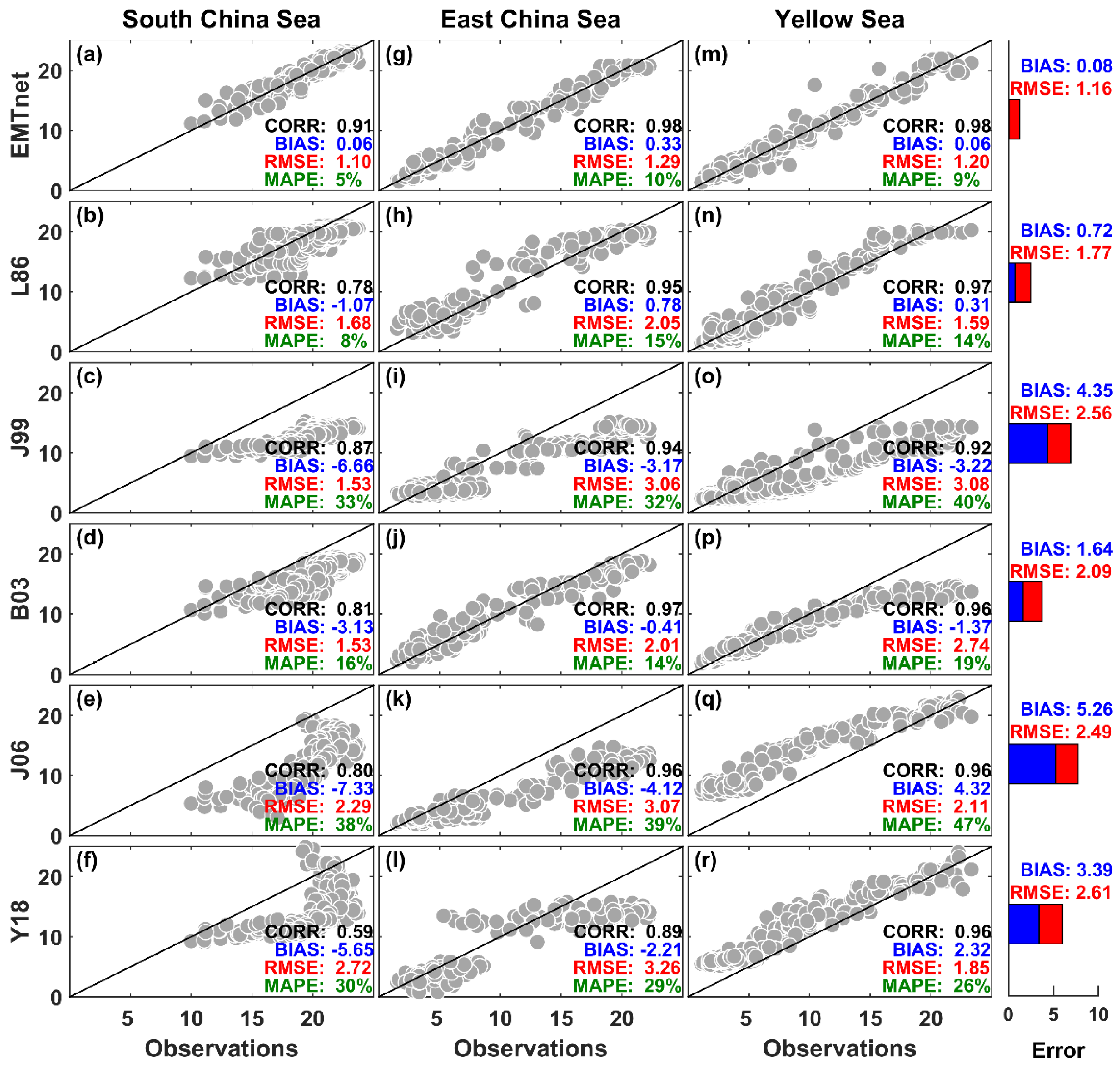
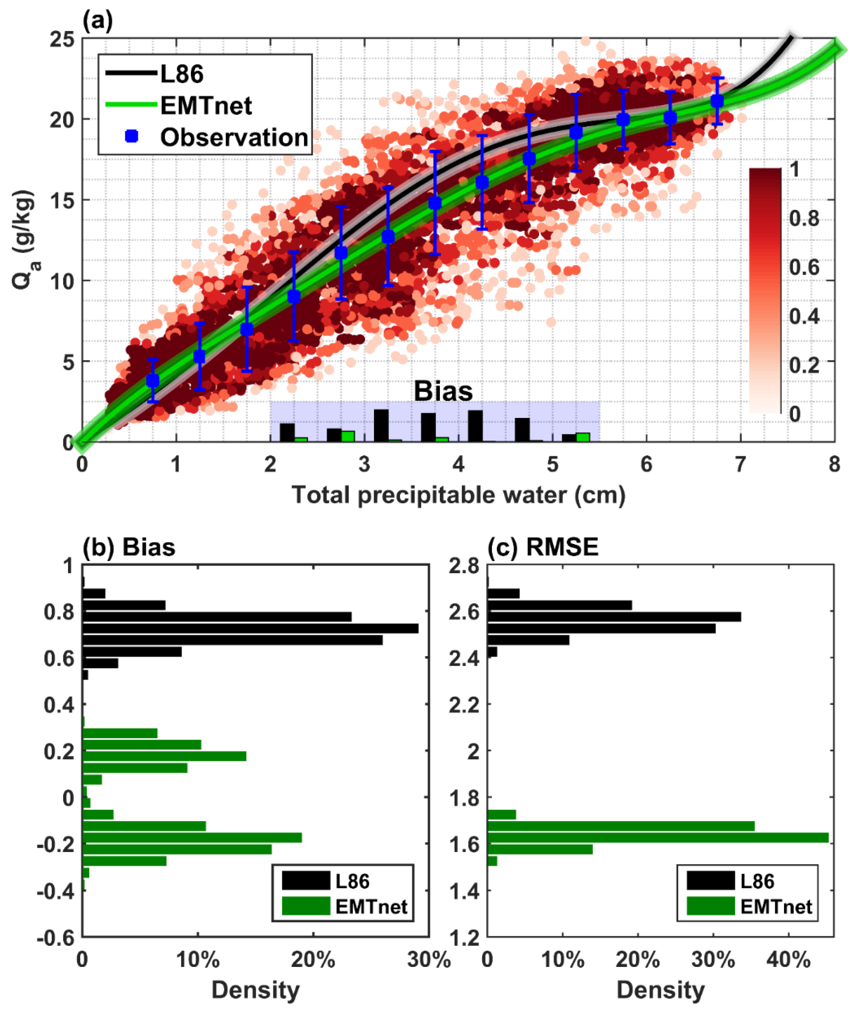
3.1. EMTnet Model Validation

The Qa predictions from the EMTnet model and five existing models are intercompared with respect to Qa observations. Three representative stations from the three China seas are selected according to their data quality, continuity, and integrity to facilitate the intercomparison. They are the Xisha Tower station in the SCS, the DH11 station in the ECS, and the HH09 station in the YS. A whole year of data from 2016 is used for each station to reduce the possible seasonal dependence of the results.
Figure 4 shows the scatter diagram between the Qa predictions and observations and the corresponding correlation coefficient (CC), mean bias, and RMSE for each model in each sea. The CCs all exceed the 99% confidence level, varying from 0.59–0.91, 0.89 to 0.98, and 0.92 to 0.98 in the SCS, ECS, and YS, respectively. Among them, the EMTnet model has the highest CCs at each station. The mean biases and RMSEs present a large spread in different models and stations. In the SCS, the EMTnet model slightly overestimates Qa by 0.06 g/kg, while the rest of the models underestimate Qa from 1.07 (L86 model) to 7.33 (Y18 model) g/kg. In the ECS, except for the EMTnet model and the L86 model which overestimate Qa by 0.13 and 0.78 g/kg, all the models underestimate Qa by 0.41 (B03 model) to 4.12 (J06 model) g/kg. In the YS, except for the J99 and B03 models which underestimate Qa by 3.22 and 1.37 g/kg, all the models overestimate Qa by 0.06 (EMTnet model) to 4.32 (J06 model) g/kg. The RMSEs of these models in the SCS, ECS, and YS are varying from 1.10 (EMTnet model) to 2.72 (Y18 model) g/kg, 1.17 (EMTnet model) to 3.36 (Y18 model) g/kg, and 1.22 (EMTnet model) to 3.08 (J99 model) g/kg.
The absolute values of the mean bias and RMSEs from the three seas are averaged for each model to compare their overall uncertainty level. The mean biases plus/minus RMSEs are 0.08 ± 1.16, 0.72 ± 1.77, 4.35 ± 2.56, 1.64 ± 2.09, 5.26 ± 2.49, and 3.39 ± 2.61 for the EMTnet, L86, J99, B03, J06, and Y18 models. Quantitatively, the EMTnet model has the lowest mean bias and RMSE on average. The EMTnet model also shows the least mean absolute percentage error (MAPE) at each station.

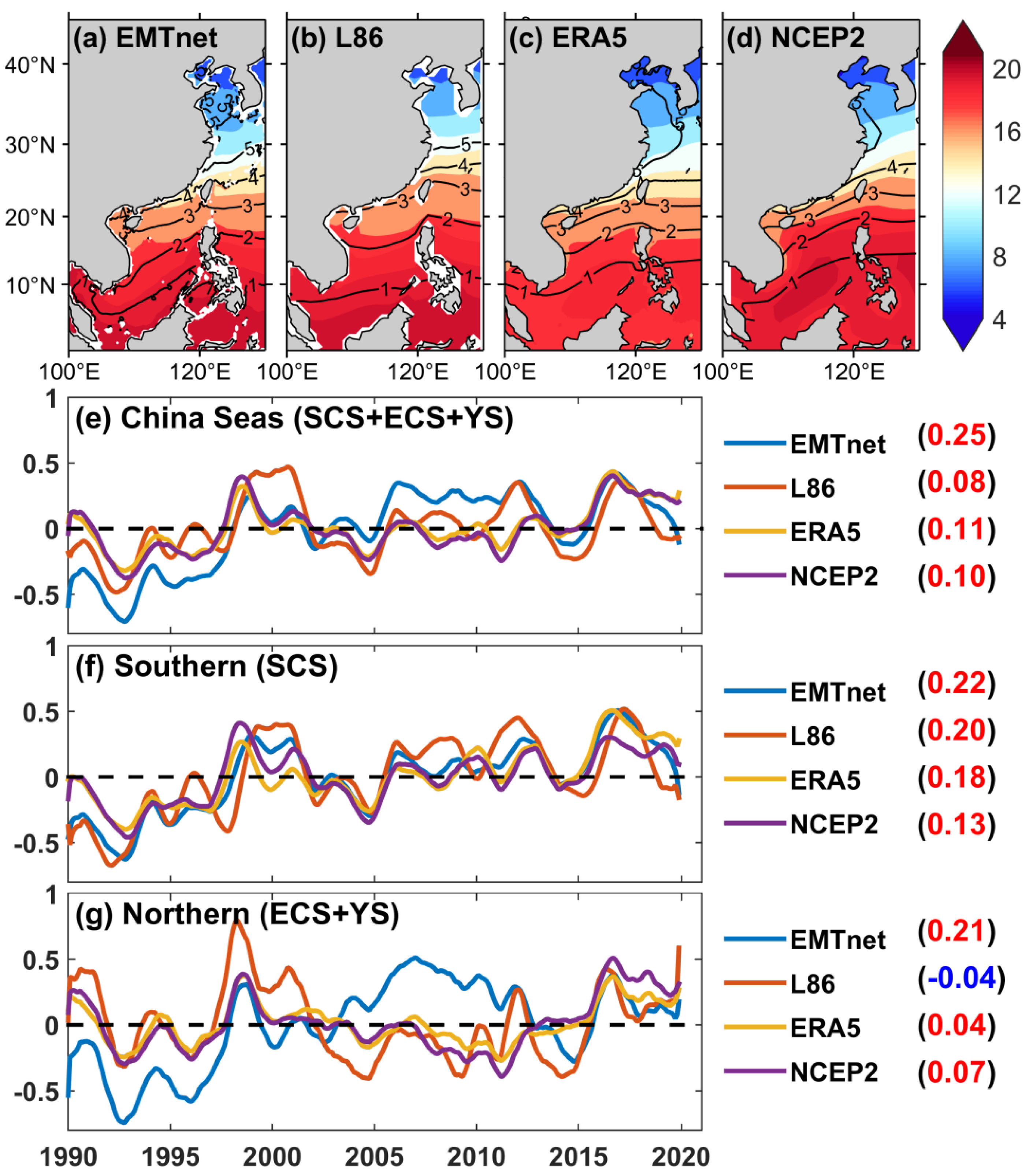
3.2. EMTnet Model Application

All the Qa observations collected here are subsequently used to fully train the EMTnet model. Qa predictions of the L86 model, which has the best performance among these five existing models, are used as a reference here. It is noted that both the EMTnet model and the L86 model take TPW as an input variable, which confirms the good relationship between TPW and Qa over the China Seas. Figure 5a compares the Qa predictions of the EMTnet model and the L86 model in the form of the QaW relation. The dots determined by Qa and TPW data cluster around the classical curve of the L86 model. The data density distribution shows that the majority of the data coincide well with the L86 model. Compared to the medians of Qa observations, however, biases of the L86 model occur primarily under moderate Qa values. For example, in the range of 10~20 g/kg, the L86 model overestimates Qa from 0.44 to 1.98 g/kg, while the biases of the EMTnet model are almost negligible.
Figure 5b,c depict the PDDs of the mean biases and RMSEs of the EMTnet model and the L86 model according to the 1000 samples of testing data used in the EMTnet model. The mean biases of the L86 model are concentrated from 0.60 to 0.80 (87% data). The mean biases of the EMTnet model have two peaks, which are around 0.10 to 0.30 g/kg and −0.10 to −0.30 g/kg. On average, the mean biases of the L86 model and the EMTnet model are 0.72 ± 0.06 and −0.02 ± 0.19 g/kg. The RMSEs of the L86 and EMTnet models are concentrated from 2.45 to 2.65 (94% data) and 1.55 to 1.70 (95% data) g/kg, which are on average 2.56 ± 0.05 g/kg and 1.64 ± 0.04 g/kg. Thus, the EMTnet model reduces the mean bias and RMSE of the L86 model by approximately 0.70 and 0.90 g/kg, respectively. The mean bias for the EMTnet model in satellite Qa retrieval is almost zero, reducing the RMSE of the L86 model by 36%.
Monthly gridded Qa data over the China Seas were produced with satellite multi-sensor inputs by applying the fully trained EMTnet model. Both the input and output data are on 0.25° × 25° gridded maps and span from 1990 to 2019. Figure 6a–d show the climatologies of Qa from two satellite Qa retrieval models (EMTnet and L86) and two reanalyses (ERA5 and NCEP2). Except for some differences in detail, apparent gradients from south to north in the mean state and seasonal variation in Qa can be observed in all four data sources, which is higher in the south and lower in the north. Here, the intensity of seasonal variations is defined by the standard deviation from January to December.
The atmosphere’s capacity to hold water vapor will increase in a warming climate according to the Clausius–Clapeyron relation [46]. The long-term trend of Qa over the China Seas is depicted in Figure 6e–g. With the global warming in recent decades, the four data sources show consistent upward trends of Qa (Figure 6e). However, the L86 model, ERA5, and NCEP2 have relatively lower climbing rates of Qa, which are 0.08, 0.11, and 0.10 g/kg per decade, compared to the results of the EMTnet model (0.23 g/kg per decade). It is found that the long-term trends of Qa are probably underestimated in both the southern (the SCS) and northern (the ECS and YS) sections, especially for the latter. In the southern section, the long-term trends of Qa are 0.22, 0.20 0.18, and 0.13 g/kg per decade in the EMTnet model, L86 model, ERA5, and NCEP2 (Figure 6f). Except for NCEP2, all the data show quite similar climbing rates of Qa. In contrast, the long-term trends of Qa show larger spread in the northern section, which are 0.21, −0.04, 0.04, and 0.07 g/kg per decade in the EMTnet model, L86 model, ERA5, and NCEP2 (Figure 6g). Therefore, the possible underestimation of upward trends of Qa in the L86 model, ERA5, and NCEP2 can be mainly attributed to their too-weak trends of Qa variations in the northern section.

4. Discussions

The interpretability of deep learning is of great significance for its development and application. The EMTnet model and the L86 model, which take TPW as an input variable, are the top two best performing models investigated here. The possible reasons why the EMTnet model can further improve the satellite Qa retrieval compared to the L86 model are discussed. Taking the result of the L86 model as a reference, eight sensitivity experiments (Exp1 to Exp8) are designed to examine whether the improvement of the EMTnet model is due to the model itself or the additional training data such as CLW, U, and SST compared to the L86 model. All the sensitivity experiments employ TPW as a fixed variable and adopt the eight combinations of CLW, U, and SST to construct their training data. Note that Exp1, including the full CLW, U, and SST information, is the result shown in Figure 5. The statistical results for Exp1 to Exp8 are shown in Table 3. As revealed in Table 3, all the experiments show improvements in satellite Qa retrieval compared to the L86 model. They reduce the mean biases and RMSEs to varying extents. If only TPW data are used as training data as in the L86 model, the absolute error is reduced by 23% (Exp8). Taking into account CLW, U, and SST, the absolute errors are reduced by 35% (Exp5), 24% (Exp6), and 42% (Exp7). The three pairwise combinations of CLW, U, and SST are considered in Exp2 to Exp4. The reductions in absolute error in Exp2 to Exp4 are 42%, 47% and 48%.
The results of Exp2 to Exp7 suggest that factors CLW, U, and SST are helpful to improve the deep learning for satellite Qu retrieval. If these three factors are superimposed together, a most significant improvement of 49% (Exp1) can be archived. The abilities of CLW, U, and SST in improving satellite Qa retrieval are probably due to their roles in reflecting the environmental information. In the following, examples of the QaW relation under different CLW, U, and SST conditions are shown in Figure 7, Figure 8 and Figure 9, respectively.
The CLW is a measure of the total liquid water contained in a cloud in a vertical column of the atmosphere. As a component of TPW, the content of CLW will undoubtedly have an impact on the determination of the QaW relation. However, none of the existing models for satellite Qa retrieval incorporate cloud information. Figure 7 shows the QaW relation under two conditions, one under CLW less than 50 μm (46% data) and the other greater than 100 μm (54% data). Note that the criterion of 50 μm here is only determined by the PDD of CLW, which ensures the data balance in both cases. Under a relatively low CLW (Figure 7a), the reference curve of the L86 model passes through most of the medians of Qa observations, presenting high consistency with observations. Under a relatively high CLW (Figure 7b), however, the reference curve of the L86 model is nearly above all the medians of the Qa observations. This result indicates that a relatively high CLW condition can interfere with the determination of the QaW relation and lead to evident overestimations in satellite Qa retrieval if no CLW information is considered.
The surface wind plays a vital role in reflecting the weather conditions near the sea surface and influencing the Qa variations. Consequently, the surface wind is expected to be a potential factor that may improve the skill of satellite Qa retrieval, which has not been considered in existing models. Figure 8 shows the QaW relation with U less than 10 m/s (90% data) and greater than 10 m/s (10% data). It can be observed that the reference curve of the L86 model fits the Qa observations well under lower to moderate U (Figure 8a). In contrast, the L86 model overestimates Qa in almost all ranges of Qa under relatively high U (Figure 8b). The different performances of the L86 model here imply that the QaW relation is sensitive to surface wind conditions. One possible reason is that the water vapor distributions in the vertical column of the atmosphere are relatively stable under relatively weak U, which is conducive to the estimation of Qa from TPW. As a portion of water vapor can be carried away by horizontal advection under relatively high U, the observed Qa will be smaller than the model-predicted Qa.
SST is an important variable that reflects information on the marine environment and underlying atmospheric surface. For example, under a relatively warm SST (Figure 9b), the predictions of the L86 model are more consistent with the observations. In contrast, Qa is overestimated in the range of Qa from 10 to 20 g/kg under rather cold SSTs (Figure 9a). A colder SST means weaker sea surface evaporation, which might lead to less actual moisture than predicted values. Therefore, it is suggested that attention should be given to the QaW relation under different SST conditions.

5. Conclusions

Previous satellite Qa retrieval models suffer significant uncertainties due to factors such as model errors, scarce in situ observations, environmental interference, and so on. In this study, a deep learning approach, the EMTnet model, is proposed to improve the satellite Qa retrieval over the China Seas. The EMTnet model is based on multiple DNNs, and the ensemble mean of target DNNs is used to produce output predictions, which can obtain more objective learning results when the observational data are quite divergent. The Qa predictions from the EMTnet model outperform five existing models by nearly eliminating the mean bias and significantly reducing the RMSE. Compared to the L86 model, which has the best performance among five existing models, the outperformance of the EMTnet model can be attributed to two aspects. Firstly, if only TPW data are used as training data as in the L86 model, the EMTnet model reduces the absolute error by 23% (Table 3). This level of improvement can be attributed to the EMTnet model itself. Secondly, if CLW, U, and SST are added, the EMTnet model reduces the absolute error by 49% (Table 3). The approximately doubled increase in absolute error reduction benefits from the good interpretability of CLW, U, and SST on the determination of the QaW relation. Note that the in situ observations are with uneven distribution in time and space, which could cause errors to the performance of the EMTnet model to a certain extent. The further development of the EMTnet model needs more in situ observations.
The fully trained EMTnet model has been applied to learn from remote sensing data to produce a 30-year monthly gridded Qa data over the China Seas. It is found that current products perform well in depicting the mean state and seasonal variations in Qa. However, they show much weaker upward trends of Qa in the context of global warming, which are less than half of the EMTnet model result. As a locally well-trained and well-validated model, the different perspectives on the long-term variations in Qa suggested by the EMTnet model may help to provide new understandings for humidity-related multi-disciplinary research over the China Seas. In addition, the EMTnet model is capable of merging Qa observations from other regions as training data, which is to be applied to more oceans globally.

Author Contributions

Conceptualization, R.Z. and X.W.; methodology, R.Z. and W.G.; validation, R.Z. and W.G.; experiment, R.Z. and W.G.; formal analysis, R.Z. and W.G.; writing—original draft preparation, R.Z.; writing—review and editing, X.W.; visualization, R.Z.; supervision, X.W.; project administration, X.W. All authors have read and agreed to the published version of the manuscript.

Funding

This work was supported by the National Key R&D Program of China (Grant No. 2017YFA0603200), the Strategic Priority Research Program of Chinese Academy of Sciences (Grant Nos. XDB42000000), the National Natural Science Foundation of China (Grant Nos. 41925024, 41906178), the Key Special Project for Introduced Talents Team of Southern Marine Science and Engineering Guangdong Laboratory (Guangzhou) (GML2019ZD0306), the Innovation Academy of South China Sea Ecology and Environmental Engineering, the Chinese Academy of Sciences (ISEE2021ZD01), and the China-Sri Lanka Joint Center for Education and Research, Chinese Academy of Sciences. Rongwang Zhang was supported by the Independent Research Project Program of State Key Laboratory of Tropical Oceanography (LTOZZ2004).

Data Availability Statement

The remote sensing data are available at Remote Sensing Systems (www.remss.com, accessed on 30 June 2022). The ERA5 and NCEP2 data are available at https://www.ecmwf.int/en/forecasts/datasets/reanalysis-datasets/era5 (accessed on 30 June 2022) and https://psl.noaa.gov/data/gridded/data.ncep.reanalysis2.html (accessed on 30 June 2022), respectively. The in situ observational data can be acquired via the link https://pan.cstcloud.cn/s/4hLRaDMoRfM (accessed on 30 June 2022). The code and datasets of the EMTnet model can be acquired via the link https://pan.cstcloud.cn/s/YjAZM1vUQOA (accessed on 30 June 2022).

Acknowledgments

We thank Jun-Yue Yan for providing the in situ data collected by the program National Key Basic Research Program of China (Grant No. 2006CB403604). Acknowledgment is given for the data support of the Xisha Marine Environment National Observation and Research Station, the Marine Meteorological Science Experiment Base at Bohe of ITMM, CMA, the Yellow Sea Ocean Observation and Research Station of OMORN, and the East China Sea Ocean Observation and Research Station of OMORN.

Conflicts of Interest

The authors declare no conflict of interest.

References

  1. Baumgartner, A.; Reichel, E. The World Water Balance; Elsevier: New York, NY, USA, 1975; p. 179. [Google Scholar]
  2. Chahine, M.T. The hydrological cycle and its influence on climate. Nature 1992, 359, 373–380. [Google Scholar] [CrossRef]
  3. Trenberth, K.E.; Smith, L.; Qian, T.; Dai, A.; Fasullo, J. Estimates of the global water budget and its annual cycle using observational and model data. J. Hydrometeorol. 2007, 8, 758–769. [Google Scholar] [CrossRef]
  4. Yu, L. Global variations in oceanic evaporation (1958–2005): The role of the changing wind Speed. J. Clim. 2007, 20, 5376–5390. [Google Scholar] [CrossRef]
  5. Lorenz, D.J.; DeWeaver, E.T.; Vimont, D.J. Evaporation change and global warming: The role of net radiation and relative humidity. J. Geophys. Res. 2010, 115, D20118. [Google Scholar] [CrossRef]
  6. Jin, X.; Yu, L.; Jackson, D.L.; Wick, G.A. An improved near-surface specific humidity and air temperature climatology for the SSM/I satellite period. J. Atmos. Ocean. Technol. 2015, 32, 412–433. [Google Scholar] [CrossRef]
  7. Tomita, H.; Kubota, M.; Cronin, M.F.; Iwasaki, S.; Konda, M.; Ichikawa, H. An assessment of surface heat fluxes from J-OFURO2 at the KEO and JKEO sites. J. Geophys. Res. 2010, 115, C03018. [Google Scholar] [CrossRef]
  8. Kinzel, J.; Fennig, K.; Schröder, M.; Andersson, A.; Bumke, K.; Hollmann, R. Decomposition of random errors inherent to HOAPS-3.2 near-surface humidity estimates using multiple triple collocation analysis. J. Atmos. Ocean. Tech. 2016, 33, 1455–1471. [Google Scholar] [CrossRef]
  9. Brunke, M.A.; Wang, Z.; Zeng, X.; Bosilovich, M.; Shie, C.-L. An assessment of the uncertainties in ocean surface turbulent fluxes in 11 reanalysis, satellite-derived, and combined global datasets. J. Clim. 2011, 24, 5469–5493. [Google Scholar] [CrossRef]
  10. Kent, E.C.; Berry, D.I.; Prytherch, J.; Roberts, J.B. A comparison of global marine surface-specific humidity datasets from in situ observations and atmospheric reanalysis. Int. J. Climatol. 2014, 34, 355–376. [Google Scholar] [CrossRef]
  11. Robertson, F.R.; Bosilovich, M.G.; Roberts, J.B.; Reichle, R.H.; Adler, R.; Ricciardulli, L.; Berg, W.; Huffman, G.J. Consistency of estimated global water cycle variations over the satellite era. J. Clim. 2014, 27, 6135–6154. [Google Scholar] [CrossRef] [Green Version]
  12. Rodell, M.; Beaudoing, H.K.; L’Ecuyer, T.S.; Olson, W.S.; Famiglietti, J.S.; Houser, P.R.; Adler, R.; Bosilovich, M.G.; Clayson, C.A.; Chambers, D.; et al. The observed state of the water cycle in the early twenty-first century. J. Clim. 2015, 28, 8289–8318. [Google Scholar] [CrossRef]
  13. Liman, J.; Schröder, M.; Fenning, K.; Andersson, A.; Hollmann, R. Uncertainty characterization of HOAPS 3.3 latent heat-flux-related parameters. Atmos. Meas. Tech. 2018, 11, 1793–1815. [Google Scholar] [CrossRef]
  14. Roberts, J.B.; Clayson, C.A.; Robertson, F.R. Improving near-surface retrievals of surface humidity over the global open oceans from passive microwave observations. Earth Space Sci. 2019, 6, 1220–1233. [Google Scholar] [CrossRef]
  15. Zhang, R.; Wang, X.; Wang, C. On the simulations of global oceanic latent heat flux in the CMIP5 multimodel ensemble. J. Clim. 2018, 31, 7111–7128. [Google Scholar] [CrossRef]
  16. Tomita, H.; Hihara, T.; Kubota, M. Improved satellite estimation of near-surface humidity using vertical water vapor profile information. Geophys. Res. Lett. 2018, 45, 899–906. [Google Scholar] [CrossRef]
  17. Liu, W.T.; Niiler, P.P. Determination of monthly mean humidity in the atmospheric surface layer over oceans from satellite data. J. Phys. Oceanogr. 1984, 14, 1451–1457. [Google Scholar] [CrossRef]
  18. Liu, W.T. Statistical relation between monthly precipitable water and surface-level humidity over global oceans. Mon. Weather Rev. 1986, 114, 1591–1602. [Google Scholar] [CrossRef]
  19. Hsu, S.A.; Blanchard, B.W. The relationship between total precipitable water and surface-level humidity over the sea surface: A further evaluation. J. Geophys. Res. 1989, 94, 14539–14545. [Google Scholar] [CrossRef]
  20. Schulz, J.; Schluessel, P.; Grassl, H. Water vapour in the atmospheric boundary layer over oceans from SSM/I measurements. Int. J. Remote Sens 1993, 14, 2773–2789. [Google Scholar] [CrossRef]
  21. Schlüssel, P.; Schanz, L.; Englisch, G. Retrieval of latent heat flux and longwave irradiance at the sea surface from SSM/I and AVHRR measurements. Adv. Space Res. 1995, 16, 107–116. [Google Scholar] [CrossRef]
  22. Chou, S.-H.; Atlas, R.M.; Shie, C.-L.; Ardizzone, J. Estimates of surface humidity and latent heat fluxes over oceans from SSM/I Data. Mon. Weather Rev. 1995, 123, 2405–2425. [Google Scholar] [CrossRef]
  23. Jones, C.; Peterson, P.; Gautier, C. A new method for deriving ocean surface specific humidity and air temperature: An artificial neural network approach. J. Appl. Meteorol. 1999, 38, 1229–1245. [Google Scholar] [CrossRef]
  24. Bentamy, A.; Katsaros, K.B.; Mestas-Nunoz, A.M.; Drennan, W.M.; Forde, E.B.; Roquet, H. Satellite estimates of wind speed and latent heat flux over the global oceans. J. Clim. 2003, 16, 637–656. [Google Scholar] [CrossRef]
  25. Jackson, D.L.; Wick, G.A.; Bates, J.J. Near-surface retrieval of air temperature and specific humidity using multi-sensor microwave satellite observations. J. Geophys. Res. 2006, 111, D10306. [Google Scholar] [CrossRef]
  26. Kubota, M.; Hihara, T. Retrieval of surface air specifific humidity over the ocean using AMSR-E measurements. Sensors 2008, 8, 8016–8026. [Google Scholar] [CrossRef]
  27. Jackson, D.L.; Wick, G.A.; Robertson, F.R. Improved multisensor approach to satellite-retrieved near-surface specific humidity observations. J. Geophys. Res. 2009, 114, D16303. [Google Scholar] [CrossRef]
  28. Yu, L.; Jin, X. A regime-dependent retrieval algorithm for near-surface air temperature and specific humidity from multi-microwave sensors. Remote Sens. Environ. 2018, 215, 199–216. [Google Scholar] [CrossRef]
  29. Gao, Q.; Wang, S.; Yang, X. Estimation of surface air specific humidity and air–sea latent heat flux using FY-3C microwave observations. Remote Sens. 2019, 11, 466. [Google Scholar] [CrossRef]
  30. Wang, D.; Zeng, L.; Li, X.; Shi, P. Validation of satellite-derived daily latent heat flux over the South China Sea, compared with observations and five products. J. Atmos. Ocean. Technol. 2013, 30, 1820–1832. [Google Scholar] [CrossRef]
  31. Wang, X.; Zhang, R.; Huang, J.; Zeng, L.; Huang, F. Biases of five latent heat flux products and their impacts on mixed-layer temperature estimates in the South China Sea. J. Geophys. Res. Oceans 2017, 122, 5088–5104. [Google Scholar] [CrossRef]
  32. Roberts, J.B.; Clayson, C.A.; Robertson, F.R.; Jackson, D.L. Predicting near-surface atmospheric variables from Special Sensor Microwave/Imager using neural networks with a first-guess approach. J. Geophys. Res. 2010, 115, D19113. [Google Scholar] [CrossRef]
  33. Reichstein, M.; Camps-Valls, G.; Stevens, B.; Juang, M.; Denzier, J.; Carvalhais, N. Prabhat Deep learning and process understanding for data-driven earth system science. Nature 2019, 566, 195–204. [Google Scholar] [CrossRef]
  34. Liu, B.; Li, X.; Zheng, G. Coastal inundation mapping from bitemporal and dual-polarization SAR imagery based on deep convolutional neural networks. J. Geophys. Res. Oceans 2019, 124, 9101–9113. [Google Scholar] [CrossRef]
  35. Li, X.; Liu, B.; Zheng, G.; Zhang, S.; Liu, Y.; Gao, L.; Liu, Y.; Zhang, B.; Wang, F. Deep-learning-based information mining from ocean remote-sensing imagery. Nat. Sci. Rev. 2020, 7, 1585–1606. [Google Scholar] [CrossRef]
  36. Wang, Y.; Li, X.; Song, J.; Li, X.; Zhong, G.; Zhang, B. Carbon sinks and variations of pCO2 in the Southern Ocean from 1998 to 2018 based on a deep learning approach. IEEE J. Sel. Top. Appl. Earth Observ. Remote Sens. 2021, 14, 3495–3503. [Google Scholar] [CrossRef]
  37. Zhang, R.; Huang, J.; Wang, X.; Zhang, J.A.; Huang, F. Effects of precipitation on sonic anemometer measurements of turbulent Fluxes in the atmospheric surface layer. J. Ocean Univ. China 2016, 15, 389–398. [Google Scholar] [CrossRef]
  38. Zhou, F.; Zhang, R.; Shi, R.; Chen, J.; He, Y.; Wang, D.; Xie, Q. Evaluation of OAFlux datasets based on in situ air–sea flux tower observations over the Yongxing Islands in 2016. Atmos. Meas. Tech. 2018, 11, 6091–6106. [Google Scholar] [CrossRef]
  39. Fairall, C.W.; Bradley, E.F.; Hare, J.E.; Grachev, A.A.; Edson, J.B. Bulk parameterization of air-sea fluxes: Updates and verification for the COARE algorithm. J. Clim. 2003, 16, 571–591. [Google Scholar] [CrossRef]
  40. Wentz, F.J. SSM/I Version-7 Calibration Report (Report Number 011012); Remote Sensing Systems: Santa Rosa, CA, USA, 2013; 46p. [Google Scholar]
  41. Zou, C.-Z.; Wang, W. Climate Algorithm Theoretical Basis Document (C-ATBD)—AMSU Radiance Fundamental Climate Data Record Derived From Integrated Microwave Inter-calibration Approach; Technical Report; NOAA: Asheville, NC, USA, 2013. [Google Scholar]
  42. Zou, C.-Z.; Hao, X. AMSU-A Brightness Temperature FCDR—Climate Algorithm Theoretical Basis Document. NOAA Climate Data Record Program CDRP-ATBD-0345, Rev. 2.0. 2016. Available online: http://www.ncdc.noaa.gov/cdr/operationalcdrs.html (accessed on 30 June 2022).
  43. Hersbach, H.; Bell, B.; Berrisford, P.; Hirahara, P.; Horanyi, S.; Munoz-Sabater, J.; Nicolas, J.; Peubey, C.; Radu, R.; Schepers, D.; et al. The ERA5 global reanalysis. Quart. J. R. Meteor. Soc. 2020, 146, 1999–2049. [Google Scholar] [CrossRef]
  44. Kanamitsu, M.; Ebisuzaki, W.; Woollen, J.; Yang, S.-K.; Hnilo, J.J.; Fiorino, M.; Potter, G.L. NCEP–DOE AMIP-II reanalysis (R-2). Bull. Am. Meteorol. Soc. 2002, 83, 1631–1644. [Google Scholar] [CrossRef] [Green Version]
  45. Rumelhart, D.E.; Hinton, G.E.; Williams, R.J. Learning internal representations by error propagation. Read. Cogn. Sci. 1988, 323, 399–421. [Google Scholar] [CrossRef]
  46. Held, I.M.; Soden, B.J. Robust responses of the hydrological cycle to global warming. J. Clim. 2006, 19, 5686–5699. [Google Scholar] [CrossRef]
Figure 1. (a) Geographical distribution of observational stations. Shading denotes the ocean depth. (bd) The PDDs of in situ observations of Qa over the SCS, ECS, and YS. (e) The mean results for all data. The range, mean value, and STD of the data in each panel are shown in blue text with unit of g/kg.
Remotesensing 14 04353 g001
Figure 2. Comparison of 3-day running averaged TPW data on 1 June 2014, from various types of sensors. (af) Sensors SSM/I F15, SSMIS F18, WindSat, AMSR, TMI, and GMI, respectively. Red dots are stations located in coastal areas. Note that different sensors have different scopes of data coverage in coastal areas.
Remotesensing 14 04353 g002
Figure 3. Architecture of the EMTnet. Each DNN_n (n = 1, 2, 3, …) uses 75% randomly sampled data from all in situ observations as training data, while the remaining 25% are used as testing data.
Remotesensing 14 04353 g003
Figure 4. Comparisons between Qa predictions (ordinate) and observations (abscissa). (af) The results for the Xisha buoy station in the SCS using the EMTnet model and five existing models summarized in Table 2. (gl) and (mr) The same as (af) but for the DH11 station in the ECS and the HH09 station in the YS, respectively. Bars on the rightmost side show the mean results of the three stations for each model. The units of mean bias and RMSE are g/kg.
Remotesensing 14 04353 g004
Figure 5. Comparisons of the EMTnet model and the L86 model. (a) The scatter diagram of Qa (ordinate) and TPW (abscissa), while the bars show the model biases. In (a), the red dot denotes the data density in each 0.5 cm bin of TPW and 0.5 g/kg bin of Qa with units of ‰. The blue square and error bar are the median and one STD of Qa observations in each 0.5 cm bin of TPW. (b,c) The PDDs of the mean bias and RMSE in 1000 sets of DNN computations. Black and green lines and bars are the results of the L86 model and the EMTnet model. The units of mean bias and RMSE are g/kg.
Remotesensing 14 04353 g005
Figure 6. (ad) Climatology of Qa distributions (shading) over the China Seas from the EMTnet, L86, ERA5, and NCEP2. Contours denote the intensity of seasonal variation, which is defined by one standard deviation from January to December on each grid. (e) The time series of Qa anomalies over the China Seas. (f,g) The same as (e) but for the southern (SCS) and northern (ECS and YS) sections of the China Seas. The time series in (eg) have been applied to 13-point running average operations. The values in parentheses denote the long-term trend of Qa during the period from 1990 to 2019 with unit of g/kg per decade. The units are g/kg.
Remotesensing 14 04353 g006
Figure 7. Scatter diagram of Qa (ordinate) and TPW (abscissa) for data under conditions of CLW (a) below and (b) above 50 μm. The black line denotes the L86 model. The red dot denotes the data density in each 0.5 cm bin of TPW and 0.5 g/kg bin of Qa with units of ‰. The blue square and error bar are the median and one STD of Qa in each bin of 0.5 cm of TPW, respectively. The bar plot is the probability density distribution of CLW, with red bars representing the data range used in the corresponding panel.
Remotesensing 14 04353 g007
Figure 8. The same as Figure 7 but for two conditions of U.
Remotesensing 14 04353 g008
Figure 9. The same as Figure 7 but for two conditions of SST.
Remotesensing 14 04353 g009
Table 1. Information on in situ observations collected in this study. The station names with prefixes “DH” and “HH” are located in the ECS and the YS, respectively. The remaining 13 stations are located in the SCS. The data span from 1998 to 2018 and the sampling intervals vary from 1 min to 30 min.
NameLocationOcean DepthTypeSampling IntervalPeriod
Maoming111.66°E, 20.75°N~100 mbuoy1 min26 May 2010–28 September 2011
Shantou117.34°E, 22.33°N~100 mbuoy1 min16 October 2010–16 May 2011
Bohe111.32°E, 21.46°N~15 moffshore platform10 min26 November 2009–15 May 2010
4 January 2011–28 April 2011
13 March 2012–3 June 2012
Xisha flux tower112.33°E, 16.83°Nislandtower1~10 min26 April 2008–6 October 2008
19 July 2013–31 January 2017
Xisha buoy112.33°E, 16.86°N~1000 mbuoy10 min19 September 2009–7 April 2013
14 May 2018–12 June 2018
Kexue 1110.26°E, 6.41°N~1300 mbuoy15 min7 May 1998–20 June 1998
Shiyan 3117.40°E, 20.60°N~1000 mbuoy15 min6 May 1998–23 June 1998
SCS1115.60°E, 8.10°N~3000 mbuoy15 min19 April 1998–29 April 1998
SCS3114.41°E, 12.98°N~4500 mbuoy15 min8 June 1998–16 June 1998
SCS3+114.00°E, 13.00°N~4000 mbuoy15 min13 April 1998–29 May 1998
QF301115.59°E, 22.28°N~100 mbuoy30 min1 March 2011–31 May 2011
QF302114.00°E, 21.50°N~100 mbuoy30 min1 March 2011–31 May 2011
QF303112.83°E, 21.12°N~100 mbuoy30 min1 March 2011–31 May 2011
DH06123.13°E, 30.72°N<100 mbuoy30 min29 March 2012–30 December 2013
DH10122.00°E, 31.37°N<100 mbuoy30 min1 September 2013–2 December 2015
DH11122.82°E, 31.00°N<100 mbuoy30 min1 January 2014–30 December 2016
DH20122.75°E, 29.75°N<100 mbuoy30 min6 November 2014–1 November 2016
HH07122.58°E, 37.01°N<100 mbuoy30 min29 March 2012–31 December 2013
HH09120.27°E, 35.90°N<100 mbuoy30 min1 January 2014–31 December 2016
HH19119.60°E, 35.42°N<100 mbuoy30 min6 November 2014–31 December 2016
Table 3. The mean bias and RMSE of each sensitivity experiment with EMTnet model. “Reference” refers to the result of the L86 model. In the nomenclature of Exp1 to Exp7, postfixes C, U, and S denote parameters CLW, U, and SST considered in the corresponding experiment, respectively. In Exp8, the postfix “none” means no additional information is considered. The percent change means the ratio of changes in absolute error compared to the reference value. The units of mean bias, RMSE, and absolute error are g/kg.
ReferenceExp1_CUSExp2_CUExp3_CSExp4_USExp5_CExp6_UExp7_SExp8_None
Bias0.72−0.020.080.13−0.05−0.31−0.22−0.08−0.18
RMSE2.561.641.811.621.641.812.281.832.36
Absolute error3.281.661.891.751.692.122.501.912.54
Percent change-−49%−42%−47%−48%−35%−24%−42%−23%
Publisher’s Note: MDPI stays neutral with regard to jurisdictional claims in published maps and institutional affiliations.

