Article

An Improved Coastal Marine Gravity Field Based on the Mean Sea Surface Height Constraint Factor Method

State Key Laboratory of Engineering in Surveying, Mapping and Remote Sensing, Wuhan University, 129 Luoyu Road, Wuhan 430070, China
*
Author to whom correspondence should be addressed.
Remote Sens. 2022, 14(16), 4125; https://doi.org/10.3390/rs14164125
Submission received: 5 July 2022 / Revised: 15 August 2022 / Accepted: 17 August 2022 / Published: 22 August 2022
(This article belongs to the Special Issue Remote Sensing Observation on Coastal Change)

Abstract

:
Construction of a high spatial resolution and high precision marine gravity field in coastal areas is constrained by the low quality and sparse coverage of altimetry data, except for limited shipborne and airborne gravity surveys. To address this problem, a mean sea surface height constraint factor (MSSHCF) method based on the ordinary kriging method and the remove-restore technique is proposed from the perspective of interpolation. In this method, the data is standardized during the interpolation process to reduce the error and mean sea surface as variables related to the marine gravity field are added to the semi-variance function in ordinary kriging to obtain a marine gravity field with a spatial resolution of 1′ × 1′. Validation experiments show that the MSSHCF method more closely agrees with the referenced SS V28, DTU17 global marine gravity models than the ordinary kriging method. Our results were further validated against shipborne data; the accuracy of the MSSHCF method is 0.13 and 0.33 mGal higher than that of the ordinary kriging method in two experimental areas. The effects of ocean depth and offshore distance on the results were also assessed. These results show that the proposed method is more accurate than the ordinary kriging method, when the distance and depth varied. Therefore, our study demonstrates that the MSSHCF method is an innovative and feasible tool for extracting gravity fields along coastal, beach, and island areas.

Graphical Abstract

1. Introduction

Accurate knowledge of the coastal gravity field is important when studying coastal ecosystem processes, as well as facilitating other off shore activities [1]. Gravity in coastal areas can be observed close to the coastline by shipborne gravity measurement, but this is costly and time-consuming [2]. Airborne methods can provide uniform measurements, but this approach might not be applicable due to the high cost [3,4,5,6]. Currently, there are two ways to improve the marine gravity field, including increasing the number of measurements and improving their quality [7]. A detailed marine gravity map of the Southern Ocean and Antarctic margin was obtained by adding high quality Geosat/ERM satellite data [8]. Meanwhile, the overall accuracy of the regional marine gravity field was improved to 5.5 mGal by using high density Geosat/GM altimeter satellite data [9]. The fusion of different satellite altimeters, especially GM altimeter satellite data types can further improve the accuracy of the marine gravity field to some extent [10,11,12,13,14,15]. Versions of the global marine gravity field calculated by fusing Cryosat-2, Envisat, and Jason-1 data achieved accuracy greater than 2 mGal in local areas [16]. In addition to the data fusion strategy, waveform retracking of satellite altimetry data, especially in the immediate vicinity of the coasts, can also increase the number and quality of measurements. At present, satellite altimeter technology leads to sparse data and low quality in coastal areas [17]. However, the use of an improved threshold re-tracker for Geosat/GM data improved the accuracy of the marine gravity field by approximately 11% within 10 km of Taiwan island [18]. Furthermore, a “Double Retracking” technique was used to process ERS-1 geodetic mission waveform data and improved the accuracy of the marine gravity field by 20% overall and by 40–50% in coastal areas [19]. In another study, Cryosat-2, Envisat, and Jason-1 satellite altimeter waveform maps were retracked for a significant improvement in the accuracy of the marine gravity field [13]. Other work has also shown that the use of the proposed fitting (also called retracking) strategy (ALES+) can improve the determination of mean sea surface at high latitudes [20], and the combination of different waveform retracking methods can also improve the accuracy of the marine gravity field to some extent, especially in coastal areas [21,22,23,24].
The interpolation method is needed along the coastal area because of a lack of real measurements. For example, a marine gravity field that meets the requirements can be generated using the Shepard interpolation method [25]. Moreover, the kriging interpolation technique is widely applied to produce geophysical maps, including gravity, a magnetic field, and sea depth topographic maps [26,27,28,29]. However, even for the same spatial resolution, varying interpolation methods make a significant difference in the accuracy of gridded marine gravity fields from the same data source [30]. Furthermore, when commonly used interpolation methods were compared, including inverse distance weighted (IDW), radial basis function (RBF), Shepard, and ordinary kriging, kriging has the highest accuracy but with an unacceptable accuracy loss in areas with sparse data density [31,32]. From the perspective of statistical analysis, adding data correlated with the predicted variables can improve the weight of the kriging predicted points [33]. Therefore, in order to improve accuracy of the gridded results, some researchers began to add variables to optimize the weights for the prediction points when executing kriging interpolation [34,35]. Using the Earth’s ellipsoid as a reference, the mean sea surface includes the geoid and the dynamic seafloor topography, commonly approximated from the marine geoid, a factor related to earth gravity estimated by geodesists and geophysicists [36]. Likewise, the mean height of the sea surface can play a role in reconstructing the marine gravity field [33]. In view of the sparse data density along coastal areas, this paper will present a way to improve the derived marine gravity field along the coast, using a mean sea surface height constraint factor (MSSHCF).
Unlike previous research, this study investigates the impact of interpolation methods on construction of high spatial resolution marine gravity field in coastal regions. The goal of our study is to develop an improved interpolation method that enhances the quality of the coastal marine gravity field. To address the quality of coastal gravity, we propose a mean sea surface height constraint factor (MSSHCF) method based on the ordinary kriging interpolation and a remove-restore technique. The proposed method introduces mean sea surface height factor as the distance in the vertical direction to improve the accuracy of the results at unknown points by optimizing the weight information of the control points and then improves the accuracy of the coastal marine gravity field. In this study, we take two local coastal areas as an example in the South China Sea (SCS) to validate the approach.

2. Materials and Methods

We proposed a mean sea surface height constraint factor (MSSHCF) method based on the ordinary kriging interpolation method. Ordinary kriging provides a more comprehensive picture of the global and local characteristics of marine gravity field fluctuations than other interpolation methods. In geo-statistics, the ordinary kriging method is a widely used estimation method, and it is usually stable in terms of spatial distribution data when gridding discrete points [37]. Furthermore, the ordinary kriging interpolation method can predict values for un-measured points using the weight information generated by the semi-variance function from the measured points. The introduction of correlation variables can improve the weighting information and then further improve the accuracy of the points to be measured. Thus, we proposed an MSSHCF method based on the ordinary kriging interpolation method to improve the accuracy of the coastal points to be measured.

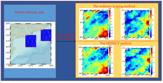
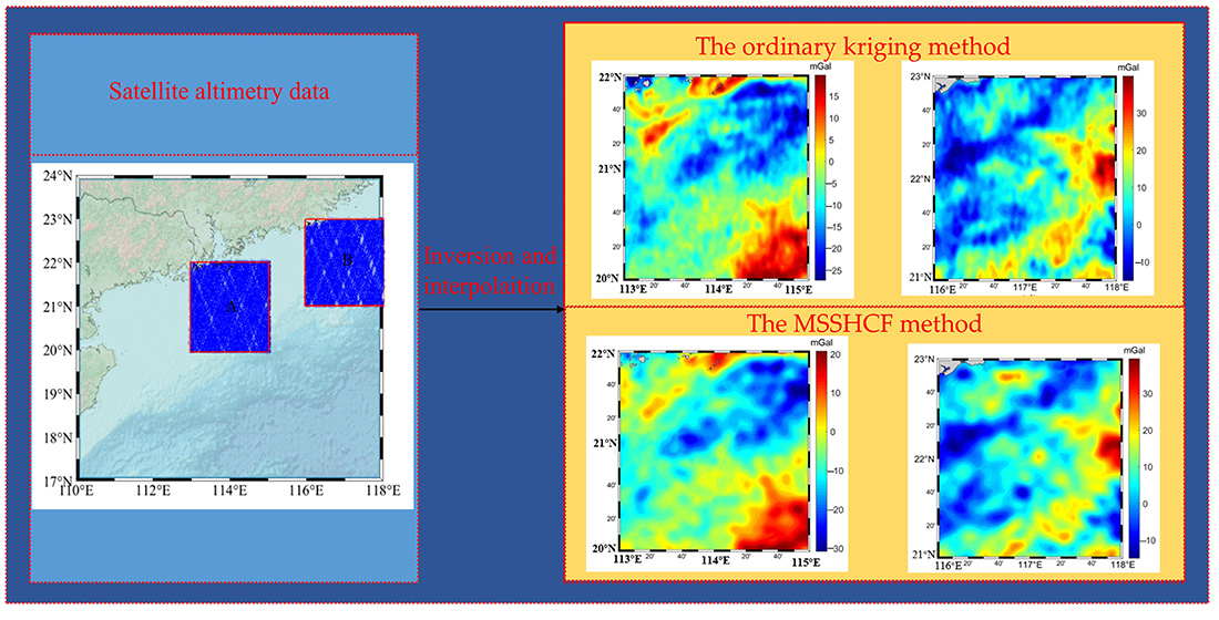
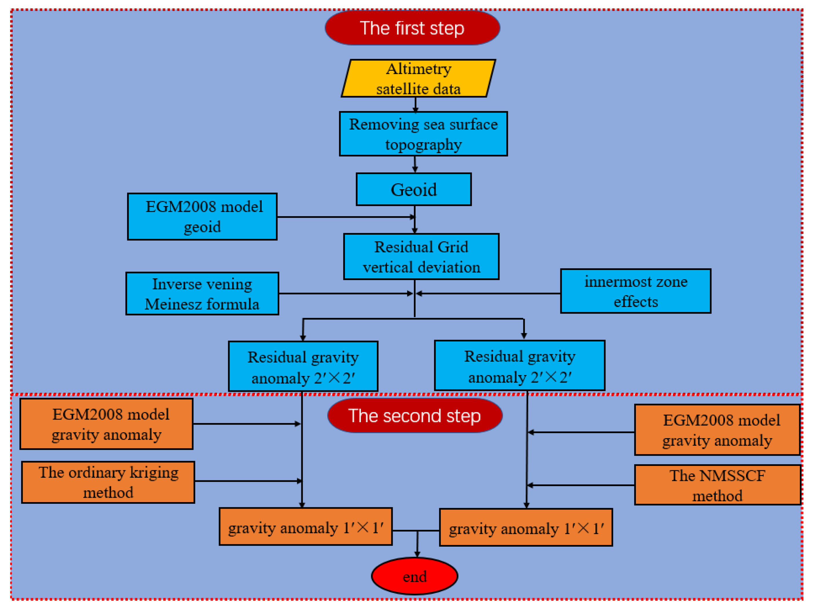
2.1. The Mean Sea Surface Height Constraints Factor (MSSHCF) Method

The methods for deriving a marine gravity field using satellite altimeter data can be broadly classified into two types: least squares configurations (LSC) and deflection of vertical (DOV). Unlike the LSC method, the DOV method can suppress long wavelength radial orbital errors below the noise level of the altimeter, using a simple gradient along the orbital geodesic [28]. We derived the marine gravity field by the Inverse Vening–Meinesz (IVM) formula based on north and east components of the deflection of vertical [38]. In order to reduce the introduction of errors while ensuring an adequate amount of gridded marine gravity data, the marine gravity field with a spatial resolution of 2-arc minute was derived for the selected region. In contrast to getting 1- and 4-arc minute marine gravity directly, this approach ensures a balance between the accuracy of the starting gravity field and the amount of computational data required for interpolation.
A high spatial resolution marine gravity field is constructed based on the principles of ordinary kriging interpolation method [29]:
G p ( x 0 , y 0 ) = i = 1 n a i ( x 0 , y 0 ) Δ g res ( x i , y i ) + g EGM   2008 ( x 0 , y 0 )
where Δ g res ( x i , y i ) is the final residual marine gravity anomaly obtained using DOV. The term g EGM   2008 denotes the reference gravity anomaly based on the EGM2008 model. The value a i ( x 0 , y 0 ) is the weight factor of known control points in the grid. The predicted values G p ( x 0 , y 0 ) in the ordinary kriging method also satisfy isotropic conditions [27]:
{ E [ Δ g res ( x 0 , y 0 ) Δ g ˜ res ( x 0 , y 0 ) ] = 0 Var [ Δ g res ( x 0 , y 0 ) Δ g ˜ res ( x 0 , y 0 ) ] = min
where Var[.] is the variance sign and Equation (2) to ensure the minimum; E[.] is the sign of the mathematical expectation of the variable. The term Δ g res ( x 0 , y 0 ) refers to the inverse gravity field residuals and Δ g ˜ res ( x 0 , y 0 ) refers to the true point gravity field residuals at the point  ( x 0 , y 0 ) . The semi-covariance function is calculated as follows:
γ ( d ) = 1 2 E [ ( Δ g ˜ res ( r ) Δ g ˜ res ( r + d ) ) 2 ]
where d is the Euclidean distance between the point ( x 0 , y 0 ) to be predicted and the current point ( x i , y i ) . The r is the position of the starting point, and γ is the semi-covariance function describing the spatial correlation of the random function. Equation (2) can be obtained based on the expected relationship between the predicted and known points:
E [ Δ g ˜ res ( x 0 , y 0 ) Δ g res ( x 0 , y 0 ) ] = E [ i = 1 n a i Δ g res ( x i , y i ) Δ g res ( x 0 , y 0 ) ] = M ( i n a i 1 )
where the M is an arbitrary constant. Based on the relationship between ( x 0 , y 0 ) and ( x i , y i ) , and according to Lagrange’s theorem, the weight coefficients a i (i = 1, 2, 3, …, n) can be obtained according to the following equation:
{ i = 1 n a i γ ij ( d ) + μ = γ j 0 ( d ) i = 1 n a i = 1
With Equation (5), the weight coefficients in the ordinary kriging method can be determined. When the mean sea surface is introduced as a constraint, the distance is redefined and calculated as follows:
{ S ij = ( x i x j ) 2 + ( y i y j ) 2 D ij = | h i h j | , ( i , j = 0 , 1 , 2 , 3 , ... , n )
where S ij and D ij are the distance variables and the variables in the vertical direction of the perpendicular face, respectively. The definition of the distance variable and the semi-variance function in the spatial domain redefined according to Equation (6) can be regained as follows [30]:
{ γ ij ( D ij , S ij ) = 1 2 ( γ ij ( D ij ) + γ ij ( S ij ) ) i = 1 n a ^ i γ ij ( D ij , S ij ) + μ = γ j 0 ( D ij , S ij ) i = 1 n λ ^ i = 1
where λ ^ i is the redetermined optimized weight factor. The values γ ij ( D ij ) and γ ij ( S ij ) are the semi-covariance functions obtained for the distance variables in Equation (6), respectively. The optimized weighting coefficients λ ^ i can be obtained by Equation (7). The values predicted by the MSSHCF method can be obtained from the following equation:
G M S S F C W ( x 0 , y 0 ) = i = 1 n λ ^ i Δ g res ( x i , y i ) + g EGM   2008 ( x 0 , y 0 )   ( i   j = 1 ,   2 ,   3 ,   ,   n )
Therefore, the inversion method of the marine gravity field is divided into two main steps: the first one is to calculate the low spatial resolution marine gravity field using the deflection of vertical method and the second step is to interpolate low spatial resolution marine gravity field using the ordinary kriging and the proposed method, i.e., to obtain a high spatial resolution marine gravity field. Before the second step is performed, the data involved in the reconstruction is simultaneously normalized to reduce errors.

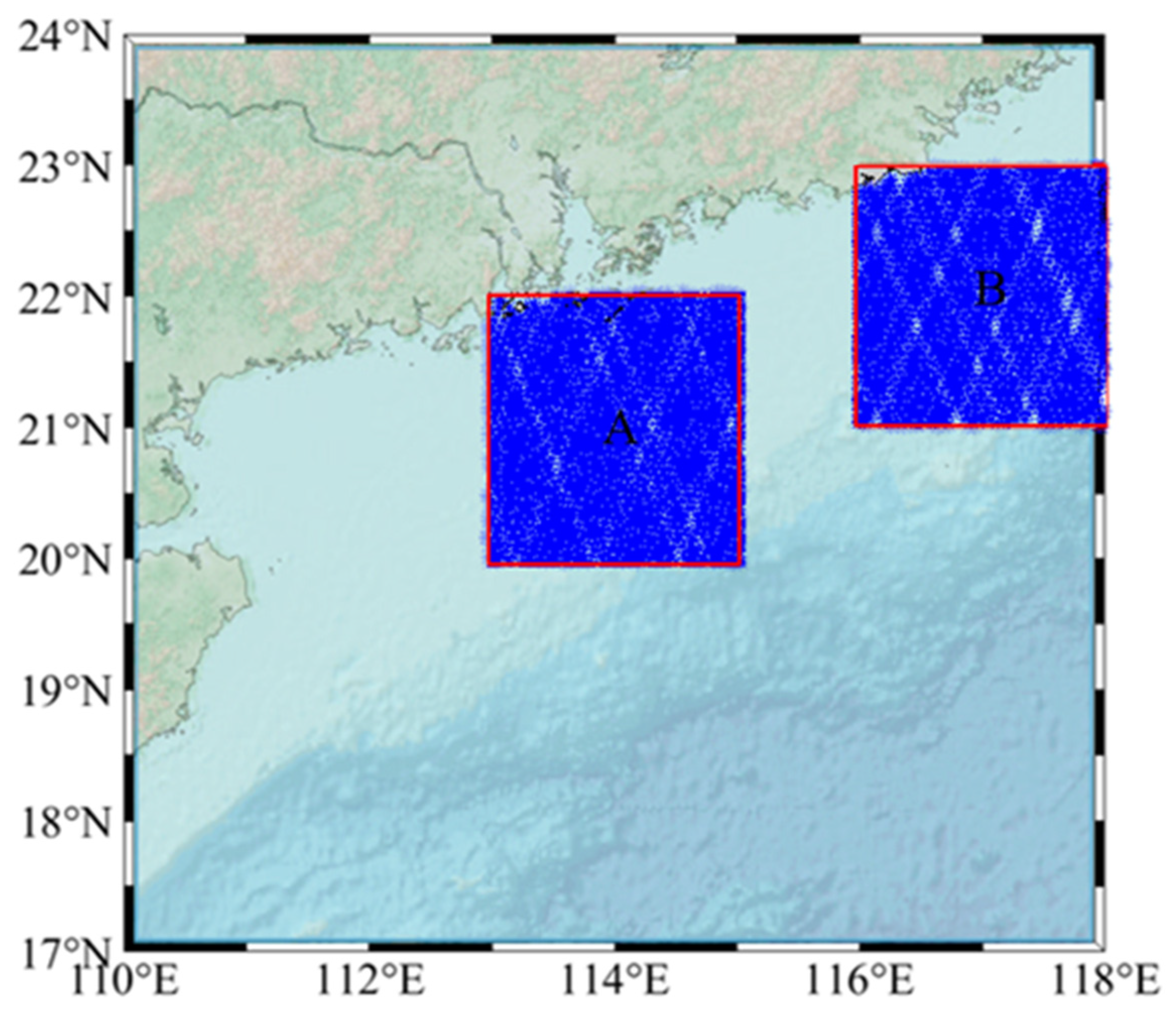
2.2. Data Preparation and Pre-Processing

Two local areas of the South China Sea (2° × 2°) are arbitrarily selected as the main experimental area A (20°~22°N, 113°E~115°E) and B (21°~23°N, 116°E~118°E). The selected areas are not only adjacent to the coast but also have a large amount of shipborne data. The satellite altimeter data sourced from Jason-1/GM is used to inverse the marine gravity field. Because the data distribution of Jason-1/GM is denser, this data provides more than three times as much geodetic missions altimetric sea surface height observations than previously available [19]. The study areas and satellite distribution trajectories are shown in Figure 1.
For the satellite altimetry data in area A and area B, we processed the data to obtain many reliable data sources before deriving the marine gravity field. The specific correction models and methods are shown in Table 1.
In Table 1, we have chosen different correction models for different errors, including the path and environmental impact errors introduced in the process of sea surface height acquisition. The ALES waveform retracking method was used to process the altimetry data to obtain more reliable data. (https://openadb.dgfi.tum.de/en/data_access/ (accessed on 27 May 2022)).

2.3. Dynamic Sea Surface Topography, Mean Sea Surface and Reference Gravity Field Model

The dynamic sea surface topography we selected was the DTU15 MDT model; it combines the gravity model EIGEN-6C4 with DTU15MSS mean sea surface model from Technical University of Denmark (DTU). Furthermore, the DTU18MSS of 1-arc minute for mean sea surface has been developed from various data sources, which contained 3 years Sentinel-3 A and the improved 7 years Cryosat-2 LRM records with a data-corrected model, which is currently the more commonly used model [39] (i.e., using FES2014 as the ocean tide model) (https://www.space.dtu.dk/ (accessed on 27 May 2022)).
The reference gravity field model plays a key role in the remove-restore technique. In our research, we used the EGM2008 global gravity field model released by the National Geospatial Intelligence Agency of the United States as a reference. The spherical harmonic expansion order of this model reached 2159, and the extended parameters extended to 2190 are also provided, which resolved the Earth’s gravity field [40] (http://icgem.gfz-potsdam.de (accessed on 27 May 2022)).

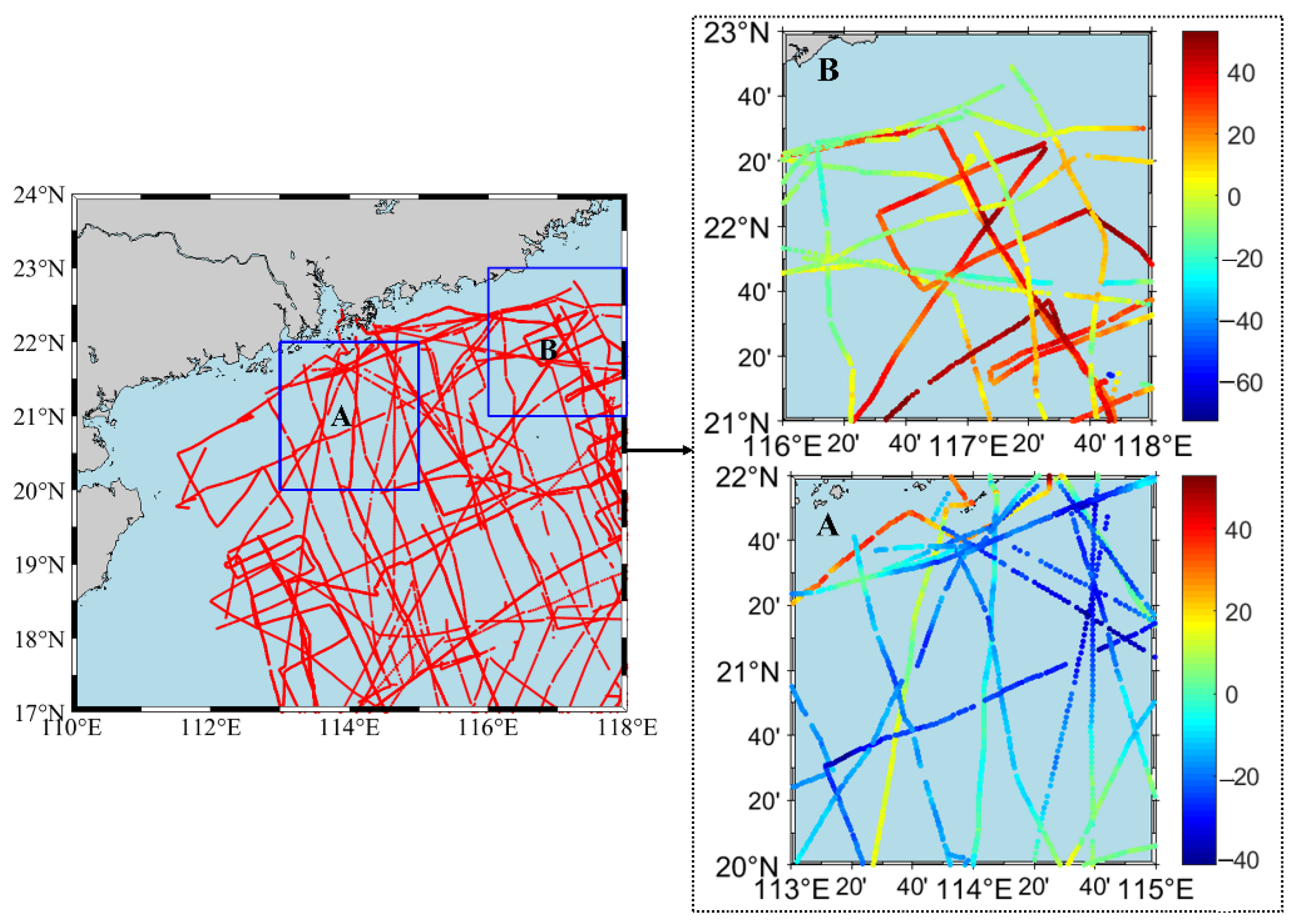
2.4. The Gravity Data Source for Comparative Verification
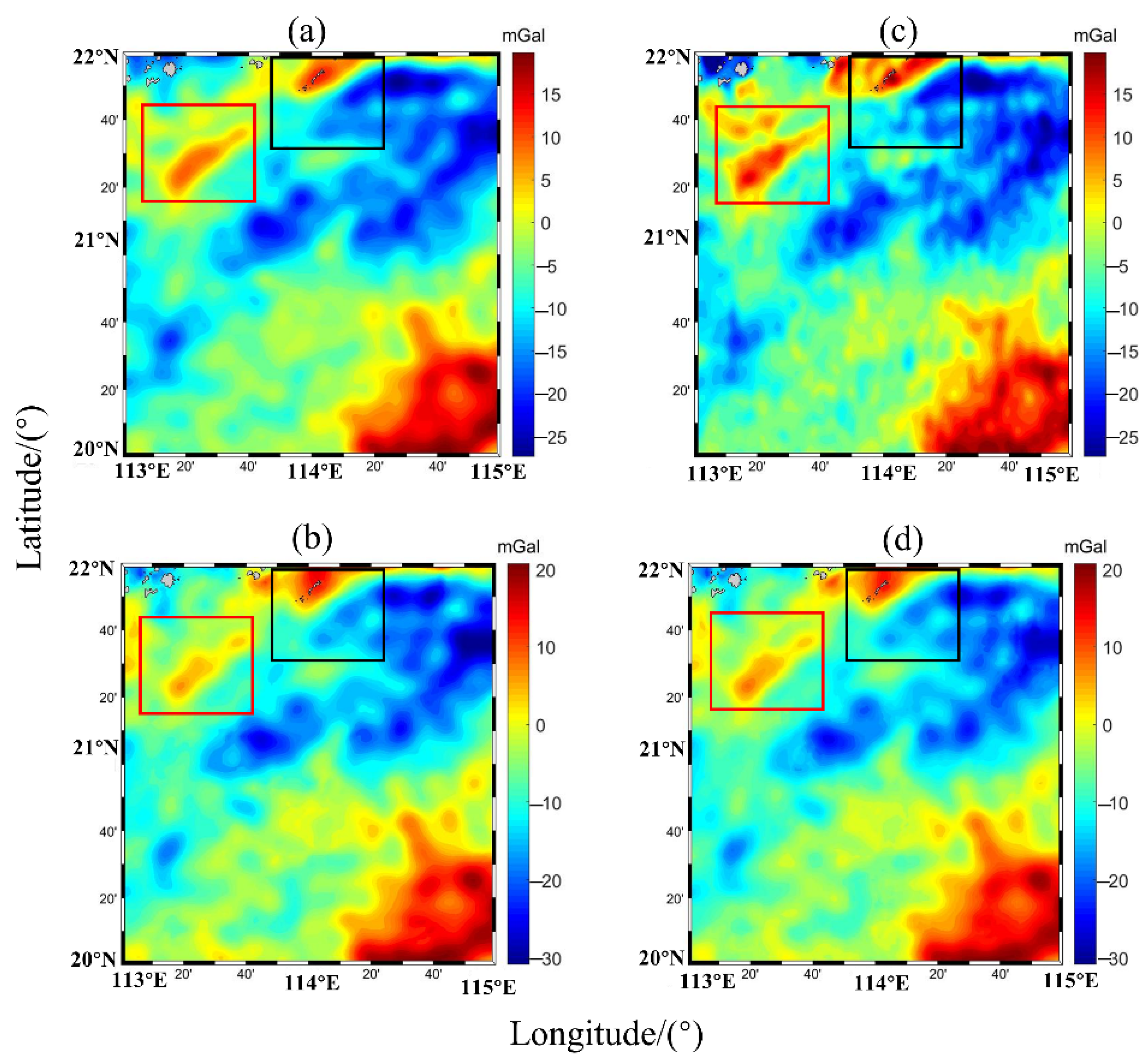
The gravity data sources for comparative verification come from two forms: global marine gravity field models and shipborne gravity data. The two marine gravity field models are DTU17 published by the Technical University of Denmark (DTU) and SS V28 published by the Scripps Institution of Oceanography (SIO), respectively. Both accurate gravity field models fused data from multiple satellite altimeters to provide the global marine gravity field values with a spatial resolution of 1′ × 1′. The shipborne gravity data comes from national geophysical data center (NGDC) [22].

3. Results

After obtaining a reliable source of satellite altimetry data, the 2-arc minute residual marine gravity field was obtained using the deflection of vertical method, and the 1-arc minute marine gravity field was obtained using the MSSHCF method, the ordinary kriging method and the EGM2008 reference gravity field model. A flow diagram showing how the 1-arc minute marine gravity reference map was acquired as shown in Figure 2. Figure 2 shows the two operations to obtain the 1-arc minute marine gravity field, including data processing, DOV, and the use of interpolation methods to obtain the final marine gravity field.
As shown, the first step consisted of data processing and the acquisition of an initial 2-arc marine gravity field by the same conditions. The second step ensured that the control conditions remained unchanged and for the normalized data to be interpolated using the proposed method and the ordinary kriging method. The results from geostatistical methods were tested by comparing the calculated values with the overlap points of the model and shipborne values. The root mean square error (RMSE) was used to assess the final results. RMSE is defined as:
R M S E = s q r t ( 1 n i n ( G M S S H C F ( X i , X i , N i ) G ( X i , X i , N i ) ) 2 ) , i = 1 , 2 , 3 ..... n
where G and G M S S H C F are the measured and predicted values, and n is the number of samples.
In the previous section, we detailed the specific process and methods used to obtain the 1′ × 1′ marine gravity field. As discussed, the MSSHCF method introduces the mean sea surface height as the weight optimization factor based on the ordinary kriging interpolation method, and the optimized weight information is used to predict unmeasured values. To compare the performance of the coastal gravity field from the ordinary kriging interpolation method and the MSSHCF method, we assessed the coastal marine gravity field using global marine gravity field models (SS V28, DTU17). The obtained final results for areas A and B and SS V28 and DTU17 marine gravity reference maps in the corresponding areas are shown in Figure 3 and Figure 4. Moreover, the corresponding final statistical results are shown in Table 2. In the black and red boxes of the marine gravity field in Figure 3 and Figure 4, we can find inconsistencies in the gravity distribution.
In Figure 3a, the distribution intervals for the DTU17 model are −27.39 to 20.80, and in Figure 3c the distribution intervals for SS V28 model are −46.63 to 21.61 mGal. Figure 3b shows a marine gravity reference map by ordinary kriging interpolation method, and it contains 14,331 points which range from −31.15 to 21.60 mGal. Figure 3d depicts the marine gravity reference map by the MSSHCF method, again containing the same amount of data with values ranging from −28.32 to 21.76 mGal. For region A, the gravity field obtained is closer to DTU17, with a larger difference in the minimum value compared with the SS V28, as can also be seen from the distribution of SS V28 in Figure 3b, but the trend of the gravity field remains unchanged. The distribution intervals from Figure 4a, c is −17.80 to 42.41 and −15.14 to 41.02 mGal, respectively. Figure 4b, d show marine gravity reference maps by the ordinary kriging and MSSHCF method, and it contains 14,224 points, which range from −15.03 to 40.49 and −15.08 to 40.55 mGal, respectively. For region B, in Figure 4, the inversion results do not vary much from the two models SS V28, DTU17, but there are still some different gravity distributions in offshore and complex regions. The final statistical results including DTU17, SS V28, EGM2008, and direct results (DR) by IVM are shown in Table 2.
Table 2 presents a comparison of the results for the tested gravity field models; we can draw the following inferences from this data. The statistical results of areas A and B in Table 2 show that when compared with the gravity field models EGM2008, DTU17, and SS V28, the Standard deviation (Std) of the MSSHCF method is more accurate than the ordinary kriging interpolation method. Furthermore, compared to the DR in region A, the Std for the ordinary Kriging interpolation and the MSSHCF methods were 9.30 and 8.78 mGal, respectively. Similarly, in region B, the Std is 9.90 for the ordinary Kriging interpolation method and 9.44 mGal for the MSSHCF method. Therefore, compared to the ordinary kriging interpolation and the MSSHCF methods, the accuracy of the gravity field obtained by using IVM directly is lower due to the sparse and low-quality data.
Scatter plots of the obtained gravity anomaly versus the global marine gravity models in areas A and B are shown in Figure 5 and Figure 6. We can see that the inversion results of the MSSHCF method and the ordinary kriging method have different coefficients of agreement with the global gravity field models.
As shown in the scatter plots for Figure 5 of area A and Figure 6 of area B, closer agreement is found between the MSSHCF method and the gravity field models, which verifies that the MSSHCF method outperforms the ordinary kriging method. Thus, the final results of MSSHCF method have a high coherence coefficient with the same global gravity field models in two regions. In contrast to the ordinary kriging method, the MSSHCF method settings were: a nested variogram consisting of two variogram function, one for the horizontal and another for the vertical direction. Under the same conditions, the weighting factor of the point to be measured can be optimized by increasing the amount of the relationship related to the oceanic gravity field. by introducing variables in the vertical direction as constraint on the gravity field. Thus, a more realistic map of the gravity distribution is possible to derive in these regions by the MSSHCF method.

4. Discussion

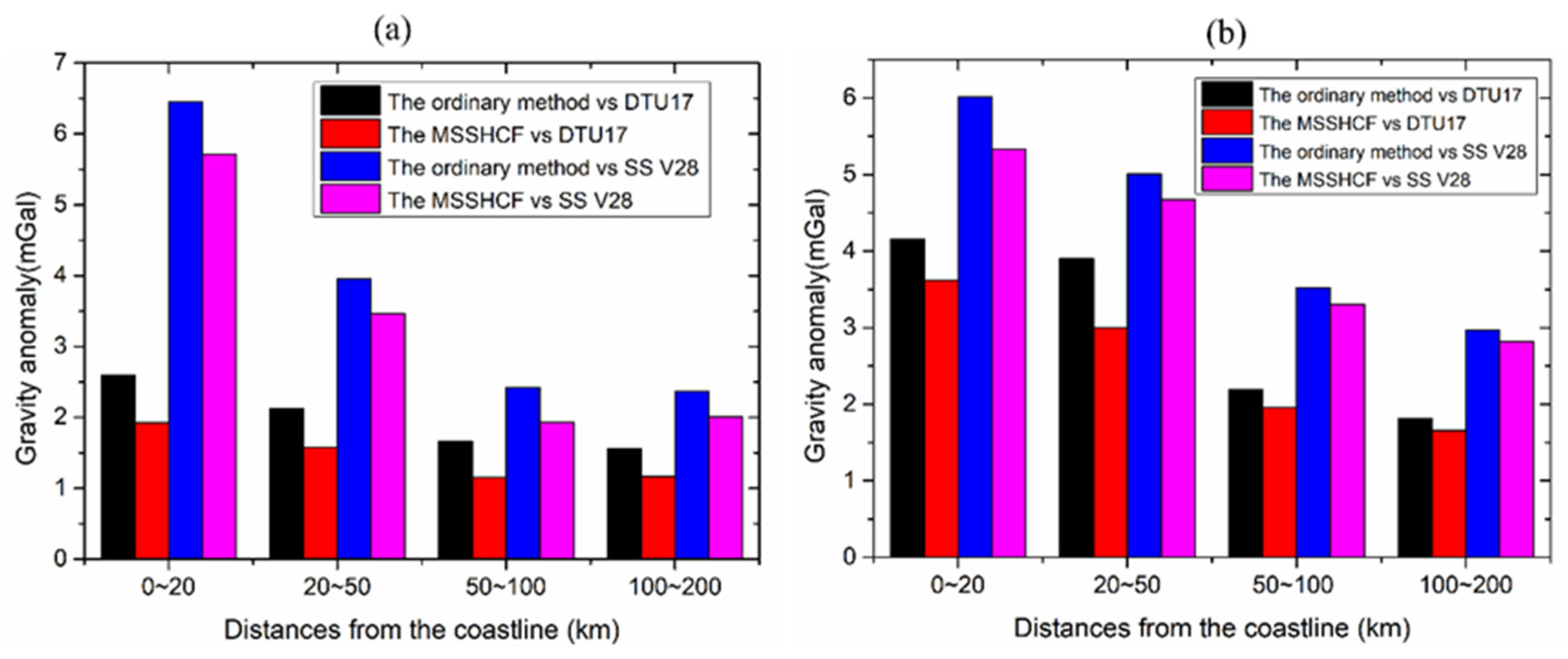
4.1. Verification from Coastal Gravity Field Models

The gravity anomaly residual maps for the corresponding locations are shown in Figure 7 and Figure 8. In the black and red boxes of the marine gravity field in Figure 7 and Figure 8, we can find some inconsistencies in the gravity residual distribution. The influence is also due precisely to the sparse amount of coastal data and the low reliability, compared to gravity field models incorporating multiple sources of data. In addition, regions with a large distribution of gravity anomaly values can be significantly different. Related research showed that there are implications for satellite altimeter inversion of the marine gravity field in some areas with significant variation in the seafloor topography [22]. In addition to the density and reliability of the satellite altimeter data, topographical factors may also lead to inconsistency in the trend of the distribution of values during the interpolation process [32]. In two figures, there are significant differences between the marine gravity fields obtained by the proposed method and the ordinary kriging method. However, excluding these data deficiencies and the topography, we find that the MSSHCF method improves the gravity field along the coast more than the ordinary kriging method.
To fully assess the performance of the two methods in coastal regions A and B, we compared the two methods with the DTU17, SS V28, and EGM2008 gravity field models and DR with varying offshore distances. The statistical results are shown in Table 3 and Table 4.
The statistical results from area A presented in Table 3 show that the proposed method improved accuracy more than the ordinary kriging method in 0 to 200 km of distance interval. The statistical results for area B in Table 4, were similar as for area A. The results in Table 3 and Table 4 also show that in the range of distances from 0 to 200 km along the coast, the accuracy of the results when directly using IVM was low when compared to results from the interpolation methods. Among these results, in the range of 0~100 km, directly using IVM had the greatest limitation on accuracy. The absolute Std results of the MSSHCF and the ordinary method after subtracting the marine gravity models are shown in Figure 9.
Figure 9a,b denote regions A and B, respectively. From the variation in Figure 9a,b, we find that as the distance changes, the inversion results are more and more accurate when compared with the gravity field models. Furthermore, when compared with the ordinary kriging method, the proposed method improves accuracy of the results more when the offshore distance is close than when the offshore distance is far. For offshore distances greater than 100 km, although the proposed method has a lower degree of improvement compared with the ordinary kriging method, it is more accurate than the ordinary method for both A and B regions. Thus, it is also demonstrated that the MSSHCF method has greater selectivity than the ordinary interpolation method in coastal areas.

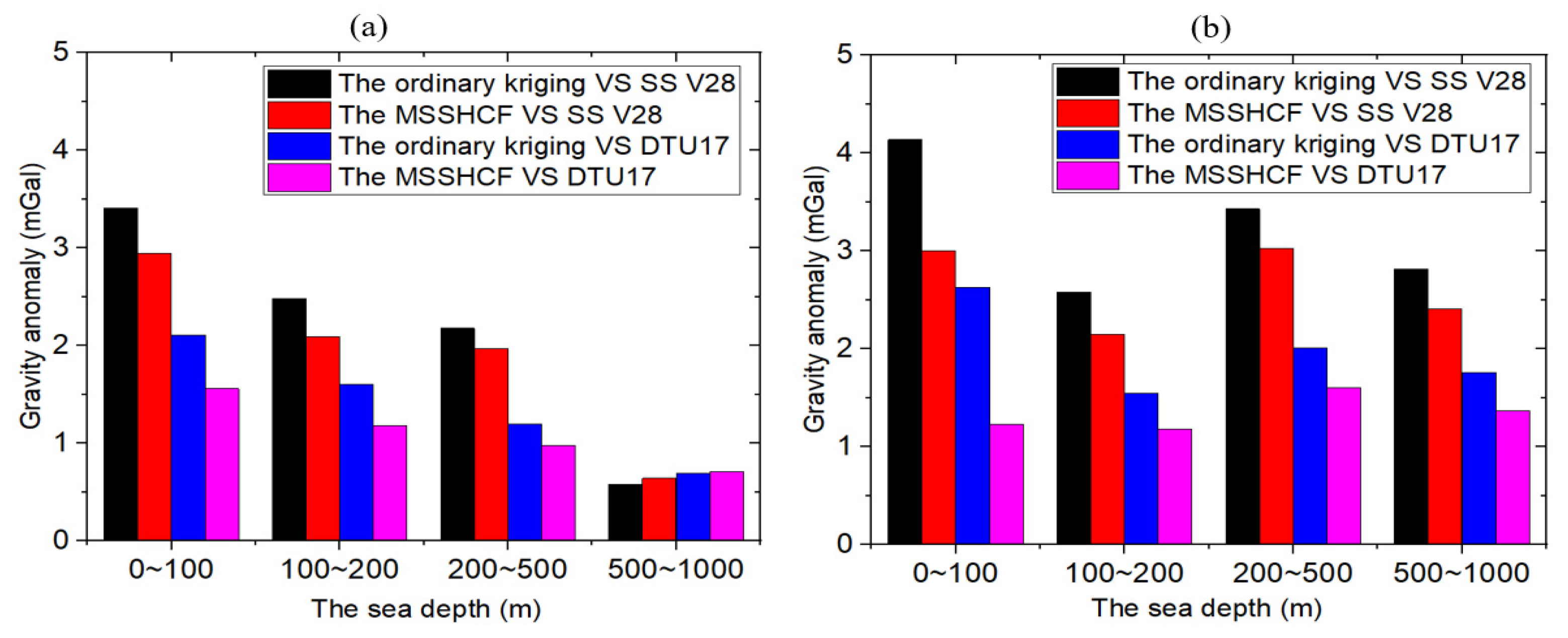
4.2. Effect of Sea Depth on Coastal Gravity Field

Different sea depth in the nearshore areas A and B were considered, and the statistical results of MSSHCF method and ordinary kriging method compared with the DTU17, SS V28, and EGM2008 gravity field models and DR at sea depths are shown in Table 5 and Table 6.
Table 5 and Table 6 show the comparative results for our research results and different gravity field models with the variations of sea depths. From the statistical results of the two tables, it can be found that with the change of sea depth, the proposed method is more accurate than the ordinary kriging method, and the accuracy of the direct results by using IVM is the least accurate. The absolute Std the results of the MSSHCF and the ordinary method after subtracting the marine gravity models at different sea depth are shown in Figure 10.
Figure 10a,b denote regions A and B, respectively. From the variation in Figure 10a, we find that accuracy of the MSSHCF method is more accurate when compared with the gravity field models at the depth of 0~500 m. Although there is little change of accuracy between 500~1000 m, the overall accuracy is still greatly improved. For Figure 10b, as the sea depth changes, the inversion results based on the MSSHCF method are the most accurate when compared with the gravity field models. Thus, compared with the ordinary method, the MSSHCF method can still optimize the coastal marine gravity field at different sea depths. We infer that this might be because the mean sea surface in the MSSHCF method is approximately equal to the ocean geodetic level, the introduction of the mean sea surface improves the prediction accuracy of the un-measured values.

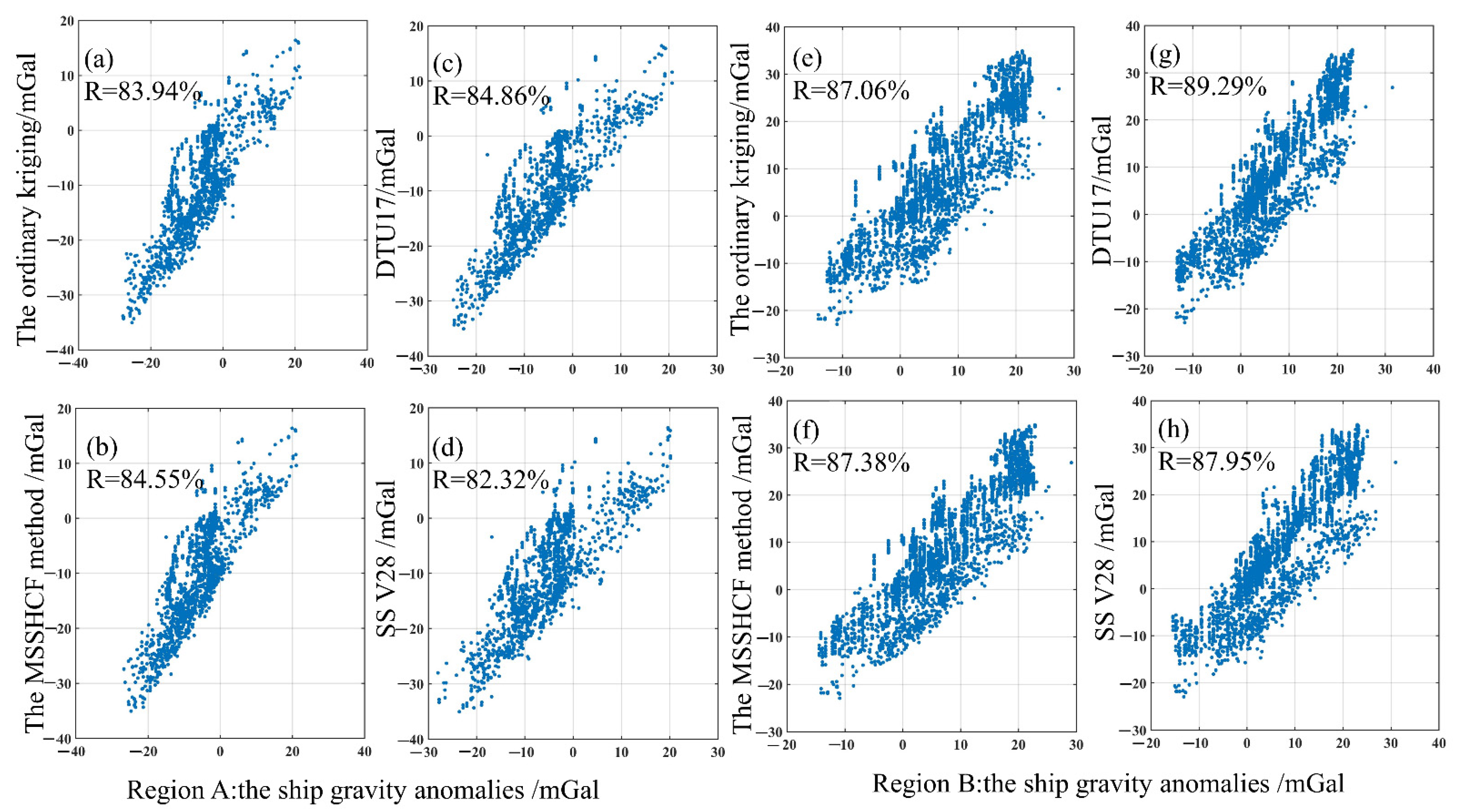
4.3. Verification against NGDC Shipboard Gravity

So far, our marine gravity field results were compared only with the current gravity field models EGM2008, SS V28, and DTU17, which was only an internal compliance test. Therefore, in external compliance tests our marine gravity field results from NMSSCF and the ordinary kriging were verified against shipborne gravity in areas A and B. The distribution of shipborne gravity in the study area is shown in Figure 11.
As shown in Figure 11, there is a relatively dense shipborne data distribution in both selected areas. There are systematic errors and outliers in the shipborne data due to the influence of sea circulation and various errors. Before using the shipboard gravity data, we processed the shipborne gravity data based on the reference Earth gravity field model EGM2008, which was used as a filter. The specific criteria were as follows: the measurement points with inconsistent values greater than 20 mGal compared with the reference gravity field model EGM2008 were eliminated for shipborne gravity data. After the systematic errors and outliers were removed, area A contained 1621 gravity data points and area B contained 3383 data points. Considering the sparsity of the shipborne data, we sampled the nearest inverse gravity data from the grid where the shipborne data was located for validation. Our marine gravity field results and the different gravity models were compared separately to shipborne gravity; the descriptive statistics are shown in Table 7.
From the results of the statistical analysis presented in Table 7, we can see that the Std of the results obtained by the MSSHCF method, the ordinary kriging method and directly by using IVM compared with the shipborne gravity are 5.39, 5.52, and 9.98 mGal in area A, respectively. When comparing the proposed MSSHCF method to the shipborne gravity, the Std of SS V28, EGM2008, and DTU17 are 5.61, 5.47, and 5.36 mGal, respectively. In Table 7, comparisons of our inversion results and shipborne gravity data show that the Std for the proposed method is almost equal to that for DTU17 and smaller than the Std for SS V28. Hence, the Std for the proposed method is smaller than that of the ordinary method. In area B, compared with the shipborne data, the Std for the proposed MSSHCF method was 5.99 mGal and for the ordinary kriging method the Std was 6.32 mGal. Compared with the ordinary kriging method, the overall accuracy of the proposed MSSHCF method in the two coastal areas was improved by 0.13 for areas A and by 0.33 mGal for area B.
We compared all gravity results with the shipborne gravity not only to verify the reasonableness of the results obtained by the MSSHCF method but also to show that it has some advantages over the ordinary kriging method. We do not deny the great advantages of global marine gravity model SS V28. However, in coastal areas with sparse data, more accuracy will be lost when the using inversion method to directly obtain the high spatial resolution marine gravity field. Therefore, it may be because the SS V28 model directly uses satellite altimetry data to derive the high spatial resolution marine gravity field in coastal areas.
Scatter plots of the gravity anomalies and shipborne gravity are shown in Figure 12. As shown in Figure 12, The overall agreement R in area A was 83.94% and the ordinary kriging method and 84.55% for the proposed MSSHCF method. In area B, there are 87.06% and 87.38% for two methods. In both areas, the agreement between the gravity field obtained by the proposed MSSHCF method and the shipborne gravity data was greater than the ordinary kriging method. Again, the results from the proposed MSSHCF method were in general agreement with the gravity field models (SS V28 and DTU17).
Using the shipborne gravity for evaluation, although the increased accuracy in the MSSHCF and the ordinary kriging method is comparatively small, it can’t be insignificant. Compared with shipborne gravity, the Std of the gravity field obtained by Zhu after fusing satellite data, such as Jason-1/2/GM, ERS-1/GM, HY-2/GM, and Cryosat-2 was 5.17 mGal [22]. However, the Std of the marine gravity field obtained by Zhu only using Jason-1/GM data is 5.79 mGal, and the overall improved accuracy is only approximately 0.6 mGal [22]. Compared with area A, although the Std of the inversion results in area B is larger than the Std of the gravity field models, this depends on the fact that we use data from only one satellite altimeter in order to validate the proposed method. However, the result also shows that the accuracy of the marine gravity field from the MSSHCF method is more accurate than the ordinary kriging method, which is closer to SS V28.
We combined the results from the proposed method with a comprehensive comparison and analysis of the shipborne coastal gravity field and the results are plausible. We only used Jason-1/GM data and did not consider other types of GM data, such as Geosat/GM, ERS-1/GM, HY-2/GM, and Cryosat-2 satellite altimeter data. However, we only verified that the proposed method is reliable for the inversion of the marine gravity field in the coastal regions, in future work more data will be considered. Our proposed approach may not be sufficiently favorable compared to the optimization of the spatial resolution and accuracy of the gravity field in coastal areas using shipborne or airborne gravity data. Numerical experiments show that the effects introduced by the proposed method appear important for coastal marine gravity optimization. Furthermore, the effects of ocean depth and offshore distance are explored in a localized 2° × 2° coastal area, which may not be rich enough to fully represent the optimization of the proposed method over the ordinary method. Here we accepted this imperfect data processing because our validation results show that the accuracy of the proposed method is more accurate with varying ocean depth and distance offshore. So, when compared with the ordinary kriging method, the proposed method has a certain degree of improvement to nearshore areas.

5. Conclusions

We investigated the effect of the interpolation methods on accuracy when inverting the high spatial resolution marine gravity fields, especially in coastal areas where altimetry data is sparse. We presented an approach based on the ordinary kriging interpolation method, which uses the mean sea surface height as the constraint component in the vertical direction to improve the weight information of the ordinary kriging method and then improved the accuracy of the un-measured values. We used the Jason-1/GM dataset with dense spatial distribution to conduct experiments in the South China Sea region. This data was subjected to error correction and waveform retracking to construct a reliable data set for the experiment [41]. In order to fully verify the validity of the method, we arbitrarily selected two coastal sub-regions with relatively dense ship data distribution; both sea and a small portion of land were included in two areas. We used the DOV method to derive the 2-arc minute residual gravity field of the experimental areas, and applied the combined MSSHCF method and the ordinary kriging method to obtain a 1-arc minute marine gravity field.
The following conclusions can be drawn. Compared to the ordinary kriging method, the experimental results show that the MSSHCF method can better assist in the construction of marine gravity fields at high spatial resolution in coastal regions. In order to fully validate the experimental results, they were evaluated in internal and external tests. The internal test used the gravity field models including the EGM2008, SS V28 and DTU17 and the external test used the shipborne gravity data. These results showed that the accuracy of the coastal marine gravity field produced by the proposed MSSHCF was improved when compared with the ordinary kriging method in two coastal areas. In addition, as the distance of the measurement values from the nearshore and its ocean depth varies, the results from the MSSHCF were more accurate than the ordinary kriging method. When the final results were evaluated with shipborne gravity, accuracy of the MSSHCF method was closer to DTU17 in area A and closer to SS V28 in area B. Thus, this is further evidence that the MSSHCF can deliver accurate coastal marine gravity field estimates in areas with sparse coastal data distribution. The validation experiments showed that the results from the proposed MSSHCF method reduces the loss of accuracy in coastal areas to some extent. This study demonstrates that the MSSHCF method is an innovative and feasible tool for the study of coastal, beach, and island areas where data are sparse and the shipborne and airborne data is lacking, and it demonstrates the validity of the proposed method in the South China Sea region.
Exploration: our results are consistent with some previous studies, where the introduction of variables related to the predicted quantity can optimize the weighting factors of the un-measured points. In order to verify the reliability of the proposed method, the single altimeter satellite data is experimented on in this paper. Thus, the fusion of data from multiple satellites to derive the marine gravity field may also have some influence on the experimental results, which will also be our next work. In addition, in the field of underwater gravity matching navigation, the proposed method can also be well applied to the reconstruction of a high spatial resolution marine gravity field map, and it has good practical significance and popularization value.

Author Contributions

Conceptualization, J.Y.; formal analysis, W.Z.; methodology, W.Z.; software, W.Z.; validation, W.Z. and J.Y.; investigation, W.Z.; resources, J.Y.; data curation, W.Z.; writing—original draft preparation, W.Z.; writing—review and editing, W.Z., J.Y. and F.L.; visualization, J.Y.; supervision, W.Z.; project administration, J.Y. and F.L.; funding acquisition, J.Y. and F.L. All authors have read and agreed to the published version of the manuscript.

Funding

This research was supported by the pre-research Project on Civil Aerospace Technologies (No. D020103) and the National Natural Science Foundation of China (42030110).

Data Availability Statement

The altimeter data for the investigated region are available from the following website: https://openadb.dgfi.tum.de/en/data_access/ (accessed on 27 May 2022) in the article under the open data source. EGM2008 can be found here: http://earth-info.nga.mil/GandG/wgs84/gravitymod/egm2008 (accessed on 27 May 2022). The NGDC shipborne data can be found here: https://maps.ngdc.noaa.gov/viewers/geophysics/ (accessed on 27 May 2022). Marine gravity: Mean Dynamic Topography and Mean Sea Surface can be obtained from the following website: https://www.space.dtu.dk/ (accessed on 27 May 2022).

Acknowledgments

The authors are thankful to the Ocean Surface Topography Science Team and its subgroup on Marine Gravity, Mean Dynamic Topography, and Mean Sea Surface for valuable discussions on the matter. All authors are thankful to the Scripps Institution of Oceanography, University of California for the marine gravity model. We are very grateful to NGDC for providing shipborne gravimetric data.

Conflicts of Interest

The authors declare no conflict of interest.

References

  1. Forsberg, R.; Olesen, A.V. Airborne Gravity Field Determination. In Sciences of Geodesy–I; Xu, G., Ed.; Springer: Berlin/Heidelberg, Germany, 2010; pp. 83–104. [Google Scholar]
  2. Claessens, S.J. Evaluation of gravity and altimetry data in Australian coastal regions. In Geodesy for Planet Earth; Kenyon, S., Pacino, C., Marti, U., Eds.; International Association of Geodesy Symposia; Springer: Berlin/Heidelberg, Germany; New York, NY, USA, 2012; Volume 136, pp. 435–442. [Google Scholar]
  3. Barzaghi, R.; Borghi, A.; Keller, K.; Forsberg, R.; Giori, I.; Loretti, I.; Olesen, A.V.; Stenseng, L. Airborne gravity tests in the Italian area to improve the geoid model of Italy. Geophys. Pros. 2009, 57, 625–632. [Google Scholar] [CrossRef]
  4. Forsberg, R.; Olesen, A.V.; Alshamsi, A.; Gidskehaug, A.; Ses, S.; Kadir, M.; Peter, B. Airborne gravimetry survey for the marine area of the United Arab Emirates. Mar. Geod. 2012, 35, 221–232. [Google Scholar] [CrossRef]
  5. Wu, Y.; Abulaitijiang, A.; Featherstone, W.E.; McCubbine, J.C.; Andersen, O.B. Coastal gravity field refinement by combining airborne and ground-based data. J. Geod. 2019, 93, 2569–2584. [Google Scholar] [CrossRef]
  6. Lu, B.; Barthelmes, F.; Li, M.; Förste, C.; Ince, E.S.; Petrovic, S.; Flechtner, F.; Schwabe, J.; Luo, Z.; Zhong, B.; et al. Shipborne gravimetry in the Baltic Sea: Data processing strategies, crucial findings and preliminary geoid determination tests. J. Geod. 2019, 93, 1059–1071. [Google Scholar] [CrossRef]
  7. Rapp, R.H. Gravity Anomalies and Sea Surface Heights Derived from a Combined GEOS 3/Seasat Altimeter Data Set. J. Geophys. Res. 1986, 91, 4867–4876. [Google Scholar] [CrossRef]
  8. Sandwell, D.; McAdoo, C. Marine gravity of the Southern Ocean and Antartic margin from Geosat. J. Geophys. Res. 1988, 93, 10389–10396. [Google Scholar] [CrossRef]
  9. Sandwell, D. Antarctic marine gravity field from high-density satellite altimetry. Geophys. J. Int. 1992, 109, 437–448. [Google Scholar]
  10. Hwang, C.; Parsons, B. An Optimal Procedure for Deriving Marine Gravity from Multi-Satellite Altimetry. Geophys. J. R. Astron. Soc. 1996, 125, 705–718. [Google Scholar] [CrossRef] [Green Version]
  11. Hwang, C.; Kao, E.; Barry, P. Global derivation of marine gravity anomalies from Marinesat, Geosat, ERS-1 and TOPEX/POSEIDON altimeter data. Geophys. J. Int. 1998, 134, 449–459. [Google Scholar] [CrossRef] [Green Version]
  12. Andersen, O.B.; Knudsen, P. Global Marine Gravity Field from the ERS-1 and Geosat Geodetic Mission Altimetry. J. Geophys. Res. 1998, 103, 8129–8137. [Google Scholar] [CrossRef]
  13. Garcia, E.S.; Sandwell, D.; Smith, H.F. Retracking CryoSat-2, Envisat and Jason-1 radar altimetry waveforms for improved gravity field recovery. Geophys. J. Int. 2014, 196, 1402–1422. [Google Scholar] [CrossRef] [Green Version]
  14. Li, Z.; Liu, X.; Guo, J.; Zhu, C.; Yuan, J.; Gao, J.; Gao, Y.; Ji, B. Performance of Jason-2/GM altimeter in deriving marine gravity with the waveform derivative retracking method: A case study in the South China Marine. Arab. J. Geosci. 2020, 13, 1–13. [Google Scholar] [CrossRef]
  15. Guo, J.; Hwang, C.; Deng, X. Editorial: Application of Satellite Altimetry in Marine Geodesy and Geophysics. Front. Earth Sci. 2022, 10, 910562. [Google Scholar] [CrossRef]
  16. Sandwell, D.T.; Garcia, E.S.; Soofi, K.; Wessel, P. Toward 1-mGal accuracy in global marine gravity from CryoSat-2, Envisat, and Jason-1. Lead. Edge 2013, 32, 892–899. [Google Scholar] [CrossRef] [Green Version]
  17. Che, D.; Li, H.; Zhang, S.; Ma, B. Calculation of Deflection of Vertical and Gravity Anomalies Over the South China Marine Derived from ICESat-2 Data. Front. Earth Sci. 2021, 9, 1–12. [Google Scholar] [CrossRef]
  18. Hwang, C.; Guo, J.; Deng, X.; Hsu, H.-Y.; Liu, Y. Coastal Gravity Anomalies from Retracked Geosat/GM Altimetry: Improvement, Limitation and the Role of Airborne Gravity Data. J. Geod. 2006, 80, 204–216. [Google Scholar] [CrossRef]
  19. Andersen, O.B.; Knudsen, P.; Berry, P. The DNSC08GRA global marine gravity field from double retracked satellite altimetry. J. Geod. 2010, 84, 191–199. [Google Scholar] [CrossRef]
  20. Passaro, M.; Kildegaard, R.; Andersen, O.B.; Boergens, E.; Calafat, F.M.; Dettmering, D.; Benveniste, J. ALES+: Adapting a homogenous marine retracker for satellite altimetry to marine ice leads, coastal and inland waters. Remote Sens. Environ. 2018, 211, 456–471. [Google Scholar] [CrossRef] [Green Version]
  21. Zhu, C.; Guo, J.; Gao, J.; Liu, X.; Hwang, C.; Yu, S.; Yuan, J.; Ji, B.; Guan, B. Marine gravity determined from multi-satellite GM/ERM altimeter data over the South China Marine: SCSGA V1.0. J. Geod. 2020, 94, 50. [Google Scholar] [CrossRef]
  22. Andersen, O.B.; Knudsen, P. The DTU17 global marine gravity field: First validation results. In International Association of Geodesy Symposia; Springer: Berlin/Heidelberg, Germany, 2019. [Google Scholar] [CrossRef]
  23. Sandwell, D.; Smith, H.F. Global marine gravity from retracked Geosat and ERS-1 altimetry: Ridge segmentation versus spreading rate. J. Geophys. Res. 2009, 114, B01411. [Google Scholar] [CrossRef] [Green Version]
  24. Tseng, K.H.; Shum, C.K.; Yi, Y.; Emery, W.J.; Kuo, C.Y.; Lee, H.; Wang, H. The Improved Retrieval of Coastal Marine Surface Heights by Retracking Modified Radar Altimetry Waveforms. IEEE Trans. Geosci. Remote Sens. 2014, 52, 991–1001. [Google Scholar] [CrossRef]
  25. Wen, H.; Jin, T.; Zhu, G.; Cheng, P. Principle and Application of Satellite Altimetry; Surveying and Mapping Press: Beijing, China, 2017; pp. 1–199. [Google Scholar]
  26. Nicolas, F.; Frédéric, M.; Michel, K. 3-Processing Geophysical Maps. Magn. Electron. 2018, 129–148. [Google Scholar] [CrossRef]
  27. Liu, Q.; Xu, K.; Jiang, M.; Wang, J. Preliminary marine gravity field from HY-2A/GM altimeter data. Acta Oceanol. Sin. 2020, 39, 127–134. [Google Scholar] [CrossRef]
  28. Zhang, Y.; Han, M.; Han, X.; Zheng, Z.; Zhai, H. Remarinerch on the applicability of Kriging method in regional gravity field interpolation. Eng. Survey Map. 2018, 27, 1–6. [Google Scholar]
  29. Li, S.; An, Z. Application of Kriging Model in Gravity Data Interpolation. Bull. Surv. Map. 2013, 10, 63–66. [Google Scholar]
  30. Kamguia, J.; Tabod, C.T.; Tadjou, J.M.; Manguelle, E.; Nouayou, R.; Kande, L.H. Accurate gravity anomaly interpolation: A case-study in Cameroon, Central Africa. Int. J. Earth Sci. 2007, 2, 108–116. [Google Scholar]
  31. Xu, Y.; Fang, Z.; Cao, W.; Huang, S.; Hao, T. Gravity anomaly reconstruction based on nonequispaced Fourier transform. Geophysics 2019, 84, G83–G92. [Google Scholar] [CrossRef]
  32. Zhang, W.; Zheng, W.; Li, Z.; Li, K.; Zhang, H. Improving the Reconstruction Accuracy of Marine Gravity Anomaly Encrypted Reference Map Using the New Mean Marine Surface 3-D Correction Method. IEEE Access 2020, 8, 214756–214774. [Google Scholar] [CrossRef]
  33. Deng, Y.; Gu, S. Spatial distribution characteristics of multipath error based on Kriging interpolation method. Sci. Survey Map. 2018, 43, 17–23. [Google Scholar]
  34. Mitchell, R.; Porth, C.B.; Porth, L.; Milton, B.; Katerina, R. Improving agricultural microinsurance by applying universal kriging and generalised additive models for interpolation of mean daily temperature. Geneva Pap. Risk Insur. Issues Pract. 2019, 44, 446–480. [Google Scholar]
  35. Ruehaak, W. 3-D interpolation of subsurface temperature data with measurement error using kriging. Environ. Earth Sci. 2015, 73, 1893–1900. [Google Scholar] [CrossRef]
  36. Nicolas, H. Defining mean sea level in military simulations with DTED. In Proceedings of the 2009 Spring Simulation Multiconference, SpringSim 2009, San Diego, CA, USA, 22–27 March 2009; Volume 115, pp. 1–3. [Google Scholar]
  37. Huang, L.; Zhang, H.; Xu, P.; Geng, J.; Wang, C.; Liu, J. Kriging with Unknown Variance Components for Regional Ionospheric Reconstruction. Sensors 2017, 17, 468. [Google Scholar] [CrossRef] [PubMed] [Green Version]
  38. Hwang, C. Inverse Vening Meinesz formula and deflection geoid formula: Application to prediction of gravity and geoid over the South China Sea. J. Geod. 1998, 72, 304–312. [Google Scholar] [CrossRef]
  39. Andersen, O.B.; Knudsen, P.; Stenseng, L. A New DTU18 MSS Mean Sea Surface–Improvement from SAR Altimetry. In Proceedings of the 25 Years of Progress in Radar Altimetry Symposium, Ponta Delgada, Portugal, 24–29 September 2018. [Google Scholar]
  40. Pavlis, N.; Holmes, S.; Kenyon, S.; Factor, J. The development and evaluation of the Earth Gravitational Model 2008(EGM2008). J. Geophys. Res. 2012, 117, B04406. [Google Scholar] [CrossRef] [Green Version]
  41. Li, Q.; Bao, L.; Wang, Y. Accuracy Evaluation of Altimeter-Derived Gravity Field Models in Offshore and Coastal Regions of China. Front. Earth Sci. 2021, 9, 722019. [Google Scholar] [CrossRef]
Figure 1. The ground track distribution of study areas from Jason-1/GM, including experimental areas A and B, respectively.
Remotesensing 14 04125 g001
Figure 2. Flow chart of 1′ marine gravity anomaly acquisition.
Remotesensing 14 04125 g002
Figure 3. The marine gravity anomaly reference maps in area A, (a) DTU17, (b) The ordinary kriging method, (c) SS V28, (d) The MSSHCF method. (Notes: The red and black squares indicate selected small areas of greater variation.).
Remotesensing 14 04125 g003
Figure 4. The marine gravity anomaly reference maps in area B, (a) DTU17, (b) The ordinary kriging method, (c) SS V28, (d) The MSSHCF method. (Notes: The red and black squares indicate selected small areas of greater variation).
Remotesensing 14 04125 g004
Figure 5. Scatter plots of gravity anomalies by the ordinary kriging interpolation method and MSSHCF method versus gravity field models in area A, (a) and (b) denote SS V28, (c) and (d) denote DTU17.
Remotesensing 14 04125 g005
Figure 6. Scatter plots of gravity anomalies by the ordinary kriging method and the MSSHCF method versus gravity field models in area B, (a,b) denote SS V28, (c,d) denote DTU17.
Remotesensing 14 04125 g006
Figure 7. The marine gravity anomaly residual maps in area A, (a) DTU17, (b) The ordinary kriging method, (c) SS V28, (d) The MSSHCF method.
Remotesensing 14 04125 g007
Figure 8. The marine gravity anomaly residual maps in area B, (a) DTU17, (b) The ordinary kriging method, (c) SS V28, (d) The MSSHCF method.
Remotesensing 14 04125 g008
Figure 9. The absolute Std of the results of the MSSHCF and the ordinary method after subtracting the gravity field models DTU17 and SS V28 at different coastal distances, (a) indicates regions A, (b) indicates region B.
Remotesensing 14 04125 g009
Figure 10. The absolute Std of the results of the MSSHCF and the ordinary method after subtracting the gravity field models DTU17 and SS V28 at different sea depth, (a) indicates regions A, (b) indicates region B.
Remotesensing 14 04125 g010
Figure 11. Shipborne gravity distribution trajectory in the study areas and the range of the shipborne gravity data in areas A and B.
Remotesensing 14 04125 g011
Figure 12. Scatter plots of gravity anomalies in areas A and B. (Notes: (ah) indicate different gravity field models and ship-borne gravity data).
Remotesensing 14 04125 g012
Table 1. Correction methods and models for obtaining sea surface height from Jason-1/GM.
CorrectionModification Model or Method
Reprocessed methodALES
Dry troposphere correctionEuropean Center for Medium Range Weather Forecasting
Wet troposphere correctionEuropean Center for Medium Range Weather Forecasting
Ionospheric correctionCNES
Marine state biasCNES
Derived barometer height correctionEuropean Center for Medium Range Weather Forecasting
High frequency fluctuations of the sea surface topographyLEGOS/CLS/CNES
Marine tideLEGOS/CNES
Load tideGOT4.10
Pole tideAviso
Table 2. Statistical results of the comparison between the marine gravity models and the final results for areas A and B (units: mGal).
RegionMethodModelMaxMinMeanStd
AThe ordinary kriging interpolation method VSSS28.32−20.2−0.833.25
DTU9.68−7.15−0.452.01
DR43.24−33.74−1.279.3
EGM20089.25−5.58−0.351.79
SS28.61−19.36−0.662.78
The MSSHCF method VSDTU8.34−5.650.281.48
DR36.13−33.87−1.098.78
EGM20087.88−6.37−0.181.29
SS15.53−13.480.3833.86
BThe ordinary kriging interpolation method VSDTU12.73−12.43−0.412.44
DR61.04−41.210.89.9
EGM200810.29−12.450.281.9
SS14.58−11.440.33.5
The MSSHCF method VSDTU9.5−6.410.332.04
DR58.74−34.450.729.44
EGM20087.79−5.830.21.44
Note: DR denotes the direct result with a spatial resolution of 1′ × 1′ by IVM.
Table 3. The statistical results of the two methods at different coastal distances, area A (units: mGal).
Distance/kmModel Comparison ResultsMaxMin MeanStd
The ordinary kriging4.07−9.02−1.522.59
The MSSHCF VS DTU173.72−7.51−1.031.92
0~20The ordinary kriging3.8−8.06−2.032.46
The MSSHCF VS EGM20084.55−7.88−1.531.99
The ordinary kriging15.84−33.89−13.939.97
The MSSHCF VS DR13.98−33.57−13.449.47
The ordinary kriging18.9−26.38−0.196.45
The MSSHCF VS SS V2818.22−26.250.35.71
The ordinary kriging6.3−5.640.92.13
The MSSHCF VS DTU174.09−4.920.571.58
20~50The ordinary kriging 4.77−7.340.581.83
The MSSHCF VS EGM20083.53−4.960.311.19
The ordinary kriging 23.4−31.360.88.9
The MSSHCF VS DR21.51−28.280.538.25
The ordinary kriging 11.95−9.291.393.96
The MSSHCF VS SS V2811.04−8.571.073.47
The ordinary kriging7.12−2.31.71.66
The MSSHCF VS DTU174.47−2.071.071.16
50~100The ordinary kriging 5.57−1.481.691.46
The MSSHCF VS EGM20085.23−0.951.041.04
The ordinary kriging33.72−10.78.387.6
The MSSHCF VS DR33.87−9.867.727.14
The ordinary kriging8.32−4.141.792.42
The MSSHCF VS SS V286.6−4.141.171.93
The ordinary kriging 5.12−5.26−0.081.56
The MSSHCF VS DTU173.53−3.45−0.071.16
100~200The ordinary kriging3.0128−4.1208−0.17921.28
The MSSHCF VS EGM20082.7119−2.9765−0.12550.9
The ordinary kriging 29.24−16.08−0.316.53
The MSSHCF VS DR29.07−14.3−0.266.14
The ordinary kriging7.82−8.290.172.37
The MSSHCF VS SS V287.38−6.680.182.01
Table 4. The statistical results of the two methods at different coastal distances, area B (units: mGal).
Distance/kmModel Comparison ResultsMaxMin MeanStd
The ordinary kriging 12.53−5.20.394.16
The MSSHCF VS DTU177.81−5.360.363.62
0~20The ordinary kriging 12.1−6.030.324.57
The MSSHCF VS EGM20085.17−4.34−0.072.49
The ordinary kriging 38.81−29.58−1.9817.11
The MSSHCF VS DR31.87−29.31−2.3715.15
The ordinary kriging14.61−9.353.076.02
The MSSHCF VS SS V2814.11−7.42.955.33
The ordinary kriging5.93−12.31−1.783.9
The MSSHCF VS DTU178.29−9.29−1.253
20~50The ordinary kriging 12.4−10.17−1.593.95
The MSSHCF VS EGM20085.52−7.79−1.252.5
The ordinary kriging 41.16−61.04−10.1618.31
The MSSHCF VS DR34.45−58.74−9.8216.98
The ordinary kriging 11.76−15.39−2.825.01
The MSSHCF VS SS V286.99−16.43−3.014.67
The ordinary kriging5.58−8.8−0.292.19
The MSSHCF VS DTU174.54−6.86−0.31.96
50~100 The ordinary kriging 3.6−6.870.11.52
The MSSHCF VS EGM20082.54−4.930.081.24
The ordinary kriging 21.34−32.711.818.02
The MSSHCF VS DR20.83−30.771.87.73
The ordinary kriging7.92−10.22−0.623.52
The MSSHCF VS SS V287.06−9.77−0.643.3
The ordinary kriging 5.12−5.83−0.271.82
The MSSHCF VS DTU174.7−5.63−0.241.65
100~200The ordinary kriging 2.61−2.01−0.261.04
The MSSHCF VS EGM20082.53−2.4−0.230.87
The ordinary kriging 13.45−10.24−0.84.99
The MSSHCF VS DR13.57−10.02−0.784.81
The ordinary kriging10.38−7.330.692.97
The MSSHCF VS SS V2810.48−6.990.712.82
Table 5. The statistical results of the two methods at different sea depth, area A (units: mGal).
Sea Depth Model Comparison ResultsMaxMin MeanStd
The ordinary kriging VS SS V2820.31−28.611.043.41
The MSSHCF VS SS V2819.36−28.590.82.95
0~100 The ordinary kriging 5.58−9.250.431.9
The MSSHCF VS EGM20086.37−7.880.211.38
The ordinary kriging 33.74−43.241.339.92
The MSSHCF VS DR33.87−36.131.119.37
The ordinary kriging VS DTU177.38−9.20.572.11
The MSSHCF VS DTU175.65−8.340.331.56
The ordinary kriging VS SS V287.82−9.260.362.48
The MSSHCF VS SS V287.77−7.650.312.09
100~200 The ordinary kriging 3.01−4.120.11.4
The MSSHCF VS EGM20083.2−3.410.081
The ordinary kriging 16.85−16.121.297
The MSSHCF VS DR16.9−15.231.266.56
The ordinary kriging VS DTU174.37−5.540.181.6
The MSSHCF VS DTU173.65−3.70.131.18
The ordinary kriging VS SS V286.46−5.37−0.482.18
The MSSHCF VS SS V286.01−5.21−0.541.97
200~500 The ordinary kriging 2.78−1.30.220.67
The MSSHCF VS EGM20081.87−0.650.190.47
The ordinary kriging 16.14−9.251.234.1
The MSSHCF VS DR14.84−8.51.23.88
The ordinary kriging VS DTU173.79−3.490.011.2
The MSSHCF VS DTU172.37−3.06−0.050.98
The ordinary kriging VS SS V28−0.49−2.5−1.380.58
500~1000 The MSSHCF VS SS V28−0.03−2.23−1.170.64
The ordinary kriging −0.12−0.69−0.420.18
The MSSHCF VS EGM2008−0.07−0.46−0.210.11
The ordinary kriging −1.54−3.05−2.30.36
The MSSHCF VS DR−1.49−2.57−2.10.32
The ordinary kriging VS DTU17−0.63−2.98−1.670.69
The MSSHCF VS DTU17−0.51−2.75−1.450.71
Table 6. The statistical results of the two methods at different sea depth, area B (units: mGal).
Sea DepthModel Comparison ResultsMaxMin MeanStd
The ordinary kriging VS DTU1712.73−12.43−1.032.63
The MSSHCF VS DTU178.29−12.31−0.431.23
0~100 mThe ordinary kriging 12.44−10.29−0.772.27
The MSSHCF VS EGM20085.83−7.79−0.571.67
The ordinary kriging 41.21−61.04−3.4111.92
The MSSHCF VS DR34.45−58.74−3.2111.34
The ordinary kriging VS SS V2813.48−15.53−1.084.14
The MSSHCF VS SS V2816.43−10.48−0.473
The ordinary kriging VS DTU175.24−4.18−0.691.55
The MSSHCF VS DTU173.8−3.94−0.231.18
100~200 mThe ordinary kriging 3.82−1.98−0.750.82
The MSSHCF VS EGM20082.53−2.24−0.590.72
The ordinary kriging 13.16−10.67−2.954.19
The MSSHCF VS DR13.46−10.98−2.84.09
The ordinary kriging VS SS V287.13−10.27−0.562.58
The MSSHCF VS SS V286.99−9.64−0.092.15
The ordinary kriging VS DTU175.96−5.830.372.01
The MSSHCF VS DTU175.29−4.750.171.6
200~500 mThe ordinary kriging 2.66−2.450.391.07
The MSSHCF VS EGM20082.81−2.170.340.93
The ordinary kriging 14.13−17.52.835.4
The MSSHCF VS DR14.86−18.022.785.25
The ordinary kriging VS SS V289.92−11.890.143.43
The MSSHCF VS SS V289.77−11.45−0.063.03
The ordinary kriging VS DTU175.54−3.11.221.76
The MSSHCF VS DTU174.13−5.120.451.37
500~1000 mThe ordinary kriging 2.62−1.970.910.93
The MSSHCF VS EGM20082.88−1.960.690.77
The ordinary kriging 14.33−6.614.974.39
The MSSHCF VS DR14.27−6.384.754.22
The ordinary kriging VS SS V2812.27−5.322.532.82
The MSSHCF VS SS V2810.14−5.241.762.41
Table 7. The Shipborne gravity comparison between the inversion results and marine gravity models in the coastal area.
AreaSource of Results MaxMinMeanStd
AThe MSSHCF method VS shipborne
gravity
13.69−15.94−4.505.39
The ordinary kriging 14.16−18.57−4.355.52
SS V28 15.74−19.74−5.195.61
DR30.74−33.74−5.849.98
EGM200812.99−12.85−4.715.47
DTU1714.97−14.65−4.925.36
BThe MSSHCF method VS shipborne
gravity
14.15−15.90−1.075.99
The ordinary kriging17.80−16.35−1.056.32
SS V28 17.55−17.11−1.205.91
DR27.66−17.42−0.516.82
EGM200813.00−12.99−1.125.84
DTU 17 15.12−17.36−1.325.83
Publisher’s Note: MDPI stays neutral with regard to jurisdictional claims in published maps and institutional affiliations.

