A Robust Sparse Imaging Algorithm Using Joint MIMO Array Manifold and Array Channel Outliers

Abstract

The multiple-input multiple-output (MIMO) radar imaging technology has attracted many scholars due to its many inherent advantages, such as avoiding complex motion compensation and imaging a quickly maneuvering target, compared to inverse synthetic aperture radar (ISAR) imaging. Although some imaging algorithms, such as the 2D fast iterative shrinkage thresholding algorithm (2D-FISTA), can meet the demand for super-resolution, they are not directly suited to MIMO radar imaging, for which the MIMO manifold needs to be considered. In this paper, based on the above questions, we propose the MIMO radar imaging algorithm, utilizing the sparsity of the scattering map in space and the MIMO array manifold, even achieving a good performance in the presence of MIMO channel error. The sparse reconstruction algorithm is developed with the alternative direction method of multipliers (ADMM) with the help of 2D-FISTA and the $l_p$-norm. Then, two algorithms are derived: one is the exact sparse recovery algorithm, and the other is the inexact sparse recovery algorithm. Although the exact sparse recovery algorithm can converge to a more accurate precision than the inexact algorithm, the latter can converge at a faster speed. Finally, the results on simulation data validated the effectiveness of the algorithm.

1. Introduction

The inverse synthetic aperture radar (ISAR) technology is an important method to estimate the distribution of moving targets in space, which utilizes the signal bandwidth and the coherent accumulation time to improve the range resolution and the cross-range resolution [1,2,3]. Interferometric ISAR (InISAR) can achieve three-dimensional (3D) imaging now, but complex image registration, motion compensation, and other algorithms need to be considered seriously in practice [4]. Compared to the imaging technology based on relative motion, real aperture radar imaging can achieve fast imaging, avoid complex motion compensation, and image a quickly maneuvering target, but real radar imaging achieves a high resolution by increasing the array aperture, which increases the hardware complexity of the system [5].

Multiple-input multiple-output (MIMO) radar imaging is one of the real aperture imaging methods. MIMO radar can achieve a higher degree of freedom by transmitting several orthogonal waveforms, these being the time-division multiplexing (TDM) signal, frequency-division multiplexing (FDM) signal, and code-division multiplexing (CDM) signal [6,7,8,9]. It can also achieve a larger array aperture compared to the traditional phased array radar (PAR). Especially, MIMO radar imaging can directly be used to image with one snapshot to avoid the complex motion compensation compared to ISAR technology, and it has attracted many scholars because of its inherent advantages with respect to ISAR imaging technology. In this paper, we researched collocated MIMO radar imaging, improving the performance by the virtual array aperture technology according to the equivalent phase center principle (PCA). Two-dimensional (2D) imaging with MIMO radar has been studied by many researchers [10,11,12]. Recently, 3D MIMO imaging methods have drawn the attention of many scholars [13,14,15]. One of the core questions is how to achieve a better resolution along with the finite array elements in MIMO radar. As the number of array elements increases, on the one hand, the resolution along with the cross-range dimension can be improved, but on the other hand, the hardware cost and the calculation amount of signal processing will simultaneously increase rapidly. The authors especially point out that compressive sensing (CS) is utilized to achieve the super-resolution of both cross-range dimensions with a finite number of array elements [15,16].

The 2D fast Fourier transform (2D-FFT) is commonly used to finish focusing along both cross-range dimensions, but the imaging resolution is poor, especially under the limited virtual aperture in MIMO radar. CS can recover a sparse signal from far fewer observed samples, which has drawn many researchers’ attention during the last decade [17]. Many sparse recovery algorithms have been derived, such as greedy iterative algorithms [18], sparse Bayesian learning (SBL) [19], convex optimization algorithms, iterative thresholding algorithms [20,21], etc. The threshold iteration algorithm is widely used in the field of signal processing because of its fast convergence and sufficient theoretical guarantee. The radar super-resolution imaging algorithm based on CS has been widely studied in synthetic aperture radar (SAR) imaging [22], ISAR imaging [23,24], and MIMO radar imaging [12,25,26] due to the sparsity of the imaging scene. However, it is essential for these imaging algorithms to make the observed matrix and grid matrix vectorized [27], which leads to the consequence that the dimension of the measurement matrix of CS is tremendously large and the computational complexity increases sharply. The 2D fast iterative shrinkage thresholding algorithm (2D-FISTA) and sequential smoothed L0 (SL0) can quickly converge, and they can achieve super-resolution withoutthe computational complexity of converting the 2D observed matrix and grid map into vectors [28,29,30]. We utilized some prior conditions, the sparsity of scattering points in space and the MIMO array manifold, to establish a new sparse imaging method in this paper. Besides, there is limited research on MIMO radar imaging in the presence of outliers, and in practice, this can be caused by radio interference, miscalibrated sensors, and other aspects of the MIMO radar system [31,32,33,34].

In this paper, we research a MIMO radar super-resolution imaging method, considering the array manifold and the outliers. We firstly reformulated the question as minimizing the $l_1$-norm and $l_p$-norm and subjecting themto the signal model. On the one hand, there is a guarantee that the targets’ location in space can be obtained by the $l_1$-norm; on the other hand, the $l_p$-norm is robust to outliers with $0<p<1$. However, the $l_p$-norm is a non-convex question, and to solve this, a complex generalized iterated shrinkage algorithm (CGISA) is developed to resist outliers in the snapshot matrix. To the best of our knowledge, we are the first to consider sparse imaging exploiting the array manifold and outlier noise in transreceivers in MIMO imaging. Comparisons with state-of-the-art algorithms show that our methods are superior in terms of robustness and resolution, and the proposed algorithm is validated on a public dataset.

This paper is organized as follows. Section 2 gives a brief introduction to the MIMO imaging model, and a detailed description of the proposed sparse recovery algorithm is given in Section 3. Section 4 gives the simulation experiments and the imaging result of the ISAR simulated data. Finally, Section 5 presents the conclusion and introduces the future work.

In this paper, we use the following notation. We use ${\parallel ·\parallel }_F$, ${\parallel ·\parallel }_1$ and ${\parallel ·\parallel }_p$ to denote the Frobenius norm, the  $l_1$-norm, and the $l_p$-norm of a matrix, respectively. The notations ${(·)}^T$, ${(·)}^H$, and ${(·)}^{-1}$ represent the transpose, the Hermitian transpose, and the inverse operation, respectively. The symbols ∇ and $tr(·)$ stand for the gradient and trace of a matrix, respectively. Boldface lower-case and upper-case letters represent vectors and matrices, respectively. $\mathfrak{K}(·)$ and $\mathfrak{I}(·)$ represent the real and imaginary parts of a complex number vector or matrix, respectively. $max(a,b)$ indicates the maximum between a and b. Finally, $\mathbb{R}$ and $\mathbb{C}$ are used to denote the set of real and complex numbers, respectively.

2. Methods

2.1. MIMO Imaging Model

Consider the MIMO radar with a 2D planar antenna array; an imaging model of it is given in Figure 1, where there are $M_t^2$ transmitted elements and $N_r^2$ received elements. The interval spaces between adjacent transmitters and receivers are $N_{r}d$ and d, respectively. The central frequency is $f_c$, and the bandwidth is B. Suppose that $M^2$ orthogonal mutually phase code modulation signals with the same center frequency and bandwidth are transmitted, and the m-th transmitted signal can be expressed by

$$\begin{array}{c}\hfill S_m\left(t\right)=A{\phi }_m\left(t\right)exp\left(j2\pi f_{c}t\right)\end{array}$$

(1)

where ${\phi }_m\left(t\right)$ denotes the phase code function, A is the amplitude of the transmit signal, and $m\in \{1,2,\cdots ,M^2\}$. Assume that there are K scatterers in the imaging scene and $\mathbf{O}$ is the imaging center. The distance between the m-th transmitted element and the k-th scattering points is $R_m^k$; the distance between the n-th received element and the k-th scattering points is $R_n^k$; then, the radar echo can be shown as

$$\begin{array}{c}\hfill \begin{array}{cc}\hfill S_n\left(t\right)=& \sum _{k=1}^K\sum _{m=1}^{M^2}{\sigma }_k{\phi }_m\left(t-{\tau }_{mn}^k\right)exp\left(-j2\pi f_c{\tau }_{mn}^k\right)\hfill \\ & (n\in \{1,2,\cdots ,N^2\})\hfill \end{array}\end{array}$$

(2)

where ${\sigma }_k$ is the backscattering coefficient and time delay ${\tau }_{mn}^k=\left(R_m^k+R_n^k\right)/c$.

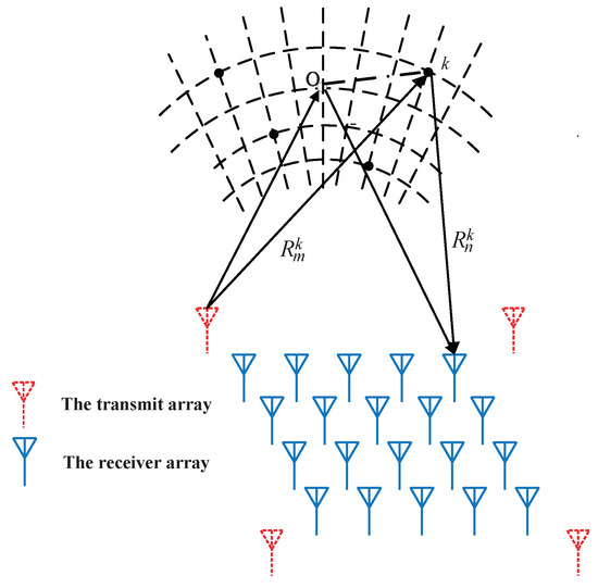
Figure 1. The MIMO radar 3D imaging model.

The echo signal can be separated into $M^2$ by a group of matched filter banks for signal $S_n\left(t\right)$, and then, the signal that the m-th transmitted element transmits and the n-th received element can be denoted as    

$$\begin{array}{c}\hfill \begin{array}{cc}\hfill S_{mn}\left(t\right)& =\sum _{k=1}^K{\sigma }_k{p}_m\left(t-\left(R_m^k+R_n^k\right)/c\right)\hfill \\ & \times exp\left(-j2\pi \left(R_m^k+R_n^k\right)/\lambda \right)\hfill \end{array}\end{array}$$

(3)

where $p(·)$ is the autocorrelation function of the m-th transmitted signal, c is the propagation velocity of the electromagnetic wave in space, and $\lambda =c/f_c$ is the wavelength of the electromagnetic wave in space.

Suppose that target scattering points in the far field are considered. The approximation conditions meet that $R_m^k+R_n^k-R_m^o-R_n^o=2{\overrightarrow{OK}}^T{\mathbf{n}}_0$, where $R_m^o$ and $R_n^o$ are the distance between the m-th transmitted element and imaging center $\mathbf{O}$ and the distance between the n-th received element and imaging center $\mathbf{O}$, respectively. ${\mathbf{n}}_0$ is a unit vector between the imaging geometry center and the array center, and it can be understood as the coordinate originof the virtual array. Then, the radar echo can be updated as

$$\begin{array}{c}\hfill \begin{array}{cc}\hfill S_n\left(t\right)& \approx \sum _{k=1}^K\sum _{m=1}^{M^2}{\sigma }_k{\phi }_m\left(t-2{\mathbf{q}}^T{\mathbf{n}}_0/c\right)\hfill \\ & \times exp\left(-j2\pi \left(R_m^k+R_n^k\right)/\lambda \right)\hfill \end{array}\end{array}$$

(4)

Based on the description in the paper [13,15], the radar echo can be rewritten as

$$\begin{array}{c}\hfill \begin{array}{cc}\hfill y_{mn}\left(t\right)& =\sum _{k=1}^K{\sigma }_{k}p\left(t-\frac{2{\mathbf{q}}^T{\mathbf{n}}_0}{c}\right)exp\left(\frac{j2\pi \Delta R}{\lambda }\right)\hfill \\ & \times exp\left(\frac{j4\pi d}{\lambda r}\left(a{x}_k+b{y}_k\right)\right)\hfill \end{array}\end{array}$$

(5)

where $\Delta R=T_{0}O+R_{0}O-T_{0}Q-R_{0}Q$ is a constant and $\mathbf{q}=\overrightarrow{OK}$. r is the distance from the imaging center O to the reference virtual element. Assume that the signal of the k-th scattering point location $\left(x_k,y_k,z_k\right)$ in space can be shown as

$$\begin{array}{c}\hfill \begin{array}{c}\hfill y_{mn}\left(t\right)=\sum _{k=1}^K\delta (t-z_k)exp\left(\frac{j4\pi da{x}_k}{\lambda r}\right)exp\left(\frac{j4\pi db{y}_k}{\lambda r}\right)\end{array}\end{array}$$

(6)

where $\delta (t-z_k)={\sigma }_{k}p\left(t-\frac{2z_k}{c}\right)$, $a,b\in \{1,2,\cdots ,MN\}$ is the row and column of the virtual array, and r is the distance from the imaging center $\mathbf{O}$ to the reference virtual element.

The 2D-FFT is employed along the cross-range of the MIMO virtual array, and the MIMO imaging model about two cross-range dimensions can be rewritten as

$$\begin{array}{c}\hfill \begin{array}{c}\hfill \mathbf{Y}=\mathbf{A}\mathbf{\Sigma }{\mathbf{B}}^T\end{array}\end{array}$$

(7)

where $\mathbf{A}$ and $\mathbf{B}$ are the overcomplete Fourier matrix, which is related to the MIMO virtual array manifold, $\mathbf{\Sigma }\in {\mathbb{C}}^{P\times Q}$ is the 2D scattering coefficients map in space, and $\mathbf{Y}$ is the snapshot matrix corresponding to the virtual array. $\mathbf{A}=\left[{\mathbf{a}}_1,{\mathbf{a}}_2,\cdots ,{\mathbf{a}}_P\right]\in {\mathbb{C}}^{M_t{N}_r\times P}$, and $\mathbf{B}=\left[{\mathbf{b}}_1,{\mathbf{b}}_2,\cdots ,{\mathbf{b}}_Q\right]\in {\mathbb{C}}^{M_t{N}_r\times Q}$, which are given by

$$\begin{array}{c}\hfill \begin{array}{c}\hfill {\mathbf{a}}_p={\left[0,exp\left(j\frac{4\pi d{x}_p}{\lambda r}\right),\cdots ,exp\left(j\frac{4\pi (M_t{N}_r-1)d{x}_p}{\lambda r}\right)\right]}^T\\ \hfill {\mathbf{b}}_q={\left[0,exp\left(j\frac{4\pi d{y}_q}{\lambda r}\right),\cdots ,exp\left(j\frac{4\pi (M_t{N}_r-1)d{y}_q}{\lambda r}\right)\right]}^T.\end{array}\end{array}$$

(8)

2.2. The Composite Optimization

Many signal processing approaches can be established as a composite optimization model, which is given by

$$\begin{array}{c}\hfill \begin{array}{c}\hfill \underset{x}{min}f\left(x\right):=g\left(x\right)+h\left(x\right)\end{array}\end{array}$$

(9)

where $g\left(x\right)$ is a convex, continuously differentiable function and $h\left(x\right)$ is a convex, continuous, but  not differentiable penalty function [20,35]. The FISTA algorithm is one of the important methods to solve optimization, and the most notable feature of this algorithm is the fast convergence speed. The FISAT algorithm is also used in low-rank matrix completion (MC), sparse recovery, and other signal processing approaches [36].

2.3. The Proposed Imaging Method

In this subsection, we clarify the signal model in the presence of outliers and provide the detailed pseudo-code of the two proposed algorithms.

Based on the above description, we exploited some prior conditions, such as the sparsity of scattering points in space, to establish the 2D sparse recovery model, in order to reduce the computational complexity and improve the effectiveness of sparse recovery. We used the fast composite optimization algorithm and threshold iteration algorithm to obtain the sparse location of scattering points. The signal model can be seen as

$$\begin{array}{c}\hfill \begin{array}{cc}\hfill & \underset{\mathbf{\Sigma }}{min}{\parallel \mathbf{\Sigma }\parallel }_0\hfill \\ & s.t.\mathbf{Y}=\mathbf{A}\mathbf{\Sigma }{\mathbf{B}}^T\hfill \end{array}\end{array}$$

(10)

(10) is a non-convex optimization problem and an NP-hard problem. In [29], the authors proposed that the above (10) can be relaxed to a convex optimization problem by the $l_1$-norm. When the impulsive signal is considered in MIMO virtual channels, the observed snapshot matrix contains some outliers. In [37], the authors pointed out that the $l_p$-norm is robust to outliers, and thereby, the $l_p$ regularization terms can be added in (10) to minimize the outliers’ error. (10) can be updated as

$$\begin{array}{c}\hfill \begin{array}{cc}\hfill & \underset{\mathbf{\Sigma }}{min}{\lambda \parallel \mathbf{\Sigma }\parallel }_1+{\parallel \mathbf{E}\parallel }_p^p\hfill \\ & s.t.\mathbf{E}=\mathbf{Y}-\mathbf{A}\mathbf{\Sigma }{\mathbf{B}}^T\hfill \end{array}\end{array}$$

(11)

where $\lambda$ is the regularization parameter and $p\in (0,1)$. The entries of $\mathbf{E}$ are expressed as

$$\begin{array}{c}\hfill \begin{array}{c}\hfill {\mathbf{E}}_{i,j}=\left\{\begin{array}{c}{\rho }_{i,j}{e}^{j{\varphi }_{i,j}},(i,j)\in \mathrm{\Omega }\\ 0,(i,j)\notin \mathrm{\Omega }\end{array}\right.\end{array}\end{array}$$

(12)

where $\mathrm{\Omega }$ denotes the entries of the outliers in the snapshot matrix and $\rho$ and $\varphi$ represent the amplitude and phase of the outliers, respectively. ${\parallel \mathbf{E}\parallel }_p^p$ can be defined as

$$\begin{array}{c}\hfill {\parallel \mathbf{E}\parallel }_p^p={\left(\sum _{i,j}{\left|E_{i,j}\right|}^p\right)}^{1/p}\end{array}$$

(13)

The optimization problem in (11) can be solved with the help of the alternative direction method of multipliers (ADMM), and the augmented Lagrangian function associated with Problem (11) is given by

$$\begin{array}{c}\hfill \begin{array}{cc}\hfill \mathcal{L}(\mathbf{\Sigma },\mathbf{E},\mathbf{R},\mu )& ={\lambda \parallel \mathbf{\Sigma }\parallel }_1+{\parallel \mathbf{E}\parallel }_p^p+\frac{\mu }{2}{\parallel \mathbf{Y}-\mathbf{A}\mathbf{\Sigma }{\mathbf{B}}^T-\mathbf{E}\parallel }_F^2\hfill \\ & +⟨\mathbf{R},\mathbf{Y}-\mathbf{A}\mathbf{\Sigma }{\mathbf{B}}^T-\mathbf{E}⟩\hfill \end{array}\end{array}$$

(14)

where $\mathbf{R}$ is the Lagrange constant and $\mu$ is a penalty coefficient. Then, the ADMM algorithm is employed to estimate the optimal variable $\mathbf{\Sigma }$, $\mathbf{E}$, $\mathbf{R}$, and $\mu$ alternately, until the convergence criterion is satisfied. Every sub-optimization problem can be formulated as

$$\begin{array}{c}\hfill \left\{\begin{array}{c}{\mathbf{\Sigma }}^{k+1}=arg\underset{\mathbf{\Sigma }}{min}\left\{\mathcal{L}\left(\mathbf{\Sigma },{\mathbf{E}}^k,{\mathbf{R}}^k,{\mu }^k\right)\right\}\hfill \\ {\mathbf{E}}^{k+1}=arg\underset{\mathbf{E}}{min}\left\{\mathcal{L}\left({\mathbf{\Sigma }}^{k+1},\mathbf{E},{\mathbf{R}}^k,{\mu }^k\right)\right\}\hfill \\ {\mathbf{R}}^{k+1}=arg\underset{\mathbf{R}}{min}\left\{\mathcal{L}\left({\mathbf{\Sigma }}^{k+1},{\mathbf{E}}^{k+1},\mathbf{R},{\mu }^k\right)\right\}\hfill \\ {\mu }^{k+1}=\rho {\mu }^k\hfill \end{array}\right.\end{array}$$

(15)

where $\rho$ is a constant to ensure the penalty coefficient $\mu$ is increasing gradually. In the next algorithmic step, we give a detailed introduction to updating every optimal variable according to the ADMM algorithm.

Updating $\mathbf{\Sigma }$

The updating of $\mathbf{\Sigma }$ can be written as

$$\begin{array}{c}\hfill \begin{array}{cc}\hfill {\mathbf{\Sigma }}^{k+1}=& arg\underset{\mathbf{\Sigma }}{min}{\lambda \parallel \mathbf{\Sigma }\parallel }_1+\frac{\mu }{2}{\parallel \mathbf{Y}-\mathbf{A}\mathbf{\Sigma }{\mathbf{B}}^T-{\mathbf{E}}^k\parallel }_F^2\hfill \\ & +⟨{\mathbf{R}}^k,\mathbf{Y}-\mathbf{A}\mathbf{\Sigma }{\mathbf{B}}^T-{\mathbf{E}}^k⟩\hfill \end{array}\end{array}$$

(16)

With some constant items omitted, the optimal variable ${\mathbf{\Sigma }}^{k+1}$ can be updated as

$$\begin{array}{c}\hfill \begin{array}{cc}\hfill {\mathbf{\Sigma }}^{k+1}& =arg\underset{\mathbf{\Sigma }}{min}{\lambda \parallel \mathbf{\Sigma }\parallel }_1+\frac{\mu }{2}{\parallel \mathbf{Y}-\mathbf{A}\mathbf{\Sigma }{\mathbf{B}}^T-{\mathbf{E}}^k+\frac{1}{\mu }{\mathbf{R}}^k\parallel }_F^2\hfill \end{array}\end{array}$$

(17)

Let ${\mathbf{D}}^k=\mathbf{Y}-{\mathbf{E}}^k+\frac{1}{{\mu }_1}{\mathbf{R}}^k$, and then, (17) can be shown in a more concise form (18).

$$\begin{array}{c}\hfill \begin{array}{cc}\hfill {\mathbf{\Sigma }}^{k+1}& =arg\underset{\mathbf{\Sigma }}{min}{\lambda \parallel \mathbf{\Sigma }\parallel }_1+\frac{\mu }{2}{\parallel {\mathbf{D}}^k-\mathbf{A}\mathbf{\Sigma }{\mathbf{B}}^T\parallel }_F^2\hfill \\ & =arg\underset{\mathbf{\Sigma }}{min}\lambda {\parallel \mathbf{\Sigma }\parallel }_1+\frac{\mu }{2}tr\left\{{\left(\mathbf{A}\mathbf{\Sigma }{\mathbf{B}}^T-{\mathbf{D}}^k\right)}^H\left(\mathbf{A}\mathbf{\Sigma }{\mathbf{B}}^T-{\mathbf{D}}^k\right)\right\}\hfill \end{array}\end{array}$$

(18)

The classical problem of the nonsmooth convex optimization model can be solved by FISTA [20]. According to the description of the composite optimization, let nonsmooth function $h\left(\mathbf{\Sigma }\right)=\lambda {\parallel \mathbf{\Sigma }\parallel }_1$ and smooth function $g\left(\mathbf{\Sigma }\right)=\frac{\mu }{2}{\parallel \mathbf{D}-\mathbf{A}\mathbf{\Sigma }{\mathbf{B}}^T\parallel }_F^2$. The gradient of $g\left(\mathbf{\Sigma }\right)$ can be written as (19).

$$\begin{array}{c}\hfill \begin{array}{cc}\hfill \nabla g\left(\mathbf{\Sigma }\right)& ={\nabla }_{\mathbf{\Sigma }}\frac{{\mu }_1}{2}\left\{tr\left(\mathbf{A}\mathbf{\Sigma }{\mathbf{B}}^T{\mathbf{B}}^{\ast }{\mathbf{\Sigma }}^H{\mathbf{A}}^H\right)-2tr\left(\mathbf{A}\mathbf{\Sigma }{\mathbf{B}}^H\left({\left({\mathbf{D}}^k\right)}^H\right)\right)\right\}\hfill \\ & =\frac{\mu }{2}\left(2{\mathbf{A}}^H\mathbf{A}\mathbf{\Sigma }{\mathbf{B}}^T{\mathbf{B}}^{\ast }-2\mathbf{A}{\mathbf{D}}^k{\mathbf{B}}^{\ast }\right)\hfill \\ & =\mu {\mathbf{A}}^H\left(\mathbf{A}\mathbf{\Sigma }{\mathbf{B}}^T-{\mathbf{D}}^k\right){\mathbf{B}}^{\ast }\hfill \end{array}\end{array}$$

(19)

To obtain the accurate target location, the temporary variable $\mathbf{X}$ is brought in, and the relationship among $\mathbf{\Sigma }$, $\mathbf{X}$, and $\nabla f\left(\mathbf{X}\right)$ can be shown as

$$\begin{array}{c}\hfill \begin{array}{c}\hfill \mathbf{\Sigma }=\underset{\mathbf{\Sigma }}{argmin}\left\{h\left(\mathbf{\Sigma }\right)+\frac{L}{2}{∥\mathbf{\Sigma }-\left(\mathbf{X}-\frac{1}{L}\nabla g\left(\mathbf{X}\right)\right)∥}_F^2\right\}\end{array}\end{array}$$

(20)

where L is the Lipschitz constant, enabling $\nabla f\left(X\right)$ to meet the Lipschitz continuity. The pseudo-code of this algorithm to obtain the sparse solution at the j-th iteration is shown in Algorithm 1, The algorithm can converge quickly with $\mathcal{O}\left(\frac{1}{j^2}\right)$, and this was demonstrated in [20]. The soft in Algorithm 1 is the soft thresholding function, which is defined as    

$$\begin{array}{c}\hfill soft(\mathbf{X},\eta )=max\left(1-\frac{\eta }{\left|\mathbf{X}\right|},0\right)\mathbf{X}.\end{array}$$

(21)

Algorithm 1 Two-dimensional sparse solution of imaging results.

Input:Convergence accuracy $ϵ$; the maximum number of iterations K; ${\mathbf{D}}^k={\mathbf{Y}}^k-{\mathbf{E}}^k+\frac{1}{{\mu }^k}{\mathbf{R}}^k$  Output: ${\mathbf{\Sigma }}^{k+1}$. 1: Initialization: 2: Initiate algorithm parameters ${\mathbf{X}}_0=\mathbf{0}$; $t_0=0$; 3: while (1) do 4:    ${\mathbf{F}}_{j+1}={\mathbf{X}}_j-\frac{1}{L}\nabla g\left({\mathbf{X}}_j\right)$ 5:    ${\mathbf{\Sigma }}_{j+1}^k=soft({\mathbf{F}}_{j+1},\frac{\lambda }{L})$ 6:    $t_{j+1}=\frac{\sqrt{1+4t_j^2}+1}{2}$ 7:    ${\mathbf{X}}_{j+1}={\mathbf{\Sigma }}_{j+1}^k+\frac{t_j-1}{t_{j+1}}\left({\mathbf{\Sigma }}_{j+1}^k-{\mathbf{\Sigma }}_j^k\right)$ 8:    if $\frac{{∥{\mathbf{\Sigma }}_{\mathbf{j}+\mathbf{1}}^{\mathbf{k}}-{\mathbf{\Sigma }}_j^k∥}_F^2}{{∥{\mathbf{\Sigma }}_{j+1}^k∥}_F^2}<ϵ$ or $j\ge K$ then 9:      ${\mathbf{\Sigma }}^{k+1}={\mathbf{\Sigma }}_{j+1}^k$; 10:      break; 11:    end if 12:    $j=j+1$ 13: end while

Updating$\mathbf{E}$

The updating of $\mathbf{E}$ can be shown as

$$\begin{array}{c}\hfill \begin{array}{cc}\hfill \mathbf{E}=& arg\underset{\mathbf{E}}{min}{\parallel \mathbf{E}\parallel }_p^p+\frac{\mu }{2}{\parallel \mathbf{Y}-\mathbf{A}{\mathbf{\Sigma }}^{k+1}{\mathbf{B}}^T-\mathbf{E}\parallel }_F^2\hfill \\ & +⟨{\mathbf{R}}^k,\mathbf{Y}-\mathbf{A}{\mathbf{\Sigma }}^{k+1}{\mathbf{B}}^T-\mathbf{E}⟩\hfill \\ & =arg\underset{\mathbf{E}}{min}{\parallel \mathbf{E}\parallel }_p^p+\frac{\mu }{2}{\parallel \mathbf{E}-\mathbf{Y}+\mathbf{A}{\mathbf{\Sigma }}^{k+1}{\mathbf{B}}^T-\frac{1}{\mu }{\mathbf{R}}^k\parallel }_F^2\hfill \end{array}\end{array}$$

(22)

Like (18), let ${\mathbf{H}}^k=\mathbf{Y}-\mathbf{A}{\mathbf{\Sigma }}^{k+1}{\mathbf{B}}^T+\frac{1}{\mu }{\mathbf{R}}^k$, and then, (22) can be defined as

$$\begin{array}{c}\hfill \mathbf{E}=arg\underset{\mathbf{E}}{min}{\parallel \mathbf{E}\parallel }_p^p+\frac{\mu }{2}{\parallel \mathbf{E}-{\mathbf{H}}^k\parallel }_F^2\end{array}$$

(23)

This is a non-convex optimization question, but fortunately, the authors proposed a generalized iterated shrinkage algorithm (GISA) for non-convex sparse coding algorithm in the paper [38], which is used to solve the $l_p$-norm optimization question. The method is easily implemented and has a good performance. However, the GISA algorithm is often used for real signals, and the radar data used for imaging are the complex signal. In this article, taking into account the characteristics of radar data, the GISA algorithm is separately performed on the real part and the imaginary part of the radar echo signal, respectively. The concrete algorithmic processing of GISTA is shown in Algorithm 2.

Then, $\mathbf{E}$ is written as

$$\begin{array}{c}\hfill \left\{\begin{array}{c}{\mathbf{H}}^k=\mathbf{Y}-\mathbf{A}{\mathbf{\Sigma }}^{k+1}{\mathbf{B}}^T+{\frac{1}{\mu }}^k{\mathbf{R}}^k\hfill \\ {\mathbf{E}}^{k+1}=CGISA\left({\mathbf{H}}^k,{\mu }^k,p,J\right)\hfill \end{array}\right.\end{array}$$

(24)

Empirically, we set $J=3$, in order to balance the gap between the computational complexity and the convergence precision.

Algorithm 2 Signal processing of CGISA.

Input signal: $\mathbf{x}\in {\mathbb{C}}^{M\times N}$, $\lambda$, p, J  Output signal: $\mathbf{y}\in {\mathbb{C}}^{M\times N}$. 1: Initialization: 2: ${\mathbf{x}}_1=\mathfrak{R}\left(\mathbf{x}\right)$; ${\mathbf{x}}_2=\mathfrak{I}\left(\mathbf{x}\right)$; ${\mathbf{y}}_1=zeros(M,N)$; ${\mathbf{y}}_2=zeros(M,N)$ 3: ${\tau }_p={\left(2\lambda (1-p)\right)}^{\frac{1}{2-p}}+\lambda p{\left(2\lambda (1-p)\right)}^{\frac{p-1}{2-p}}$ 4: for $i=1$ to J do 5:    if $|{\mathbf{x}}_i|<{\tau }_p$ then 6:      ${\mathrm{\Omega }}_i=find\left(\right|{\mathbf{x}}_i|\le {\tau }_p)$; ${\mathbf{y}}_i\left({\mathrm{\Omega }}_i\right)=0$; 7:    else 8:      $k=0,{\mathbf{x}}_i^k=\left|{\mathbf{y}}_i\right|$ 9:      while (1) do 10:         ${\mathbf{x}}_i^{k+1}=\left|{\mathbf{y}}_i\right|-\lambda p{\left({\mathbf{x}}_i^k\right)}^{p-1}$; 11:         $k=k+1$ 12:         if $k\ge J$ then 13:           break; 14:         end if 15:      end while 16:    end if 17:    $\overline{{\mathrm{\Omega }}_i}=find\left(\right|{\mathbf{x}}_i|>{\tau }_p)$; ${\mathbf{y}}_i\left(\overline{{\mathrm{\Omega }}_i}\right)=sgn\left({\mathbf{x}}_i^k\left(\overline{{\mathrm{\Omega }}_i}\right)\right){\mathbf{x}}_i^k\left({\mathrm{\Omega }}_i\right)$ 18: end for

Updating Lagrange multiplier $\mathbf{R}$ and penalty coefficient $\mu$

Lagrange multiplier $\mathbf{R}$ and Lagrange penalty parameter $\mu$ can be updated as follows:

$$\begin{array}{c}\hfill \left\{\begin{array}{c}{\mathbf{R}}^{k+1}=\mathbf{Y}-\mathbf{A}{\mathbf{\Sigma }}^{k+1}{\mathbf{B}}^T-{\mathbf{E}}^{k+1}\hfill \\ {\mu }^{k+1}=\rho {\mu }^k\hfill \end{array}\right.\end{array}$$

(25)

The pseudo-code of the proposed super-resolution imaging algorithm is shown in Algorithm 3, called the exact sparse recovery algorithm. It will consume much times, and we extended the algorithm in Algorithm 3 to the algorithm in Algorithm 4, which is dubbed the inexact sparse recovery algorithm. Compared to the exact sparse recovery algorithm, the inexact algorithm reduces the iterative process of $\mathbf{\Sigma }$. The algorithm was omitted in the iterative process of $\mathbf{\Sigma }$ inside the algorithm, and thereby, it can reduce the algorithm’s runtime.

Algorithm 3 The exact sparse algorithm.

Input: $\mathbf{Y}$, $\mathbf{A}$, and $\mathbf{B}$  Output: $\mathbf{\Sigma }$. 1: Initialization: 2: Initiate some parameters, ${\mathbf{\Sigma }}_0={\mathbf{X}}_0={\mathbf{0}}^{P\times Q}$, ${\mathbf{R}}_0={\mathbf{0}}^{P\times Q}$, $L>0$, $ϵ=1\times {10}^{-6}$, $\lambda >0$, ${\mu }_0>0$$\rho >0$, and the maximum iteration K. 3: while (1) do 4:    Update ${\mathbf{\Sigma }}^{k+1}$ using Algorithm 1 until it converges 5:    Update ${\mathbf{E}}^{k+1}$ with (24) 6:    Update ${\mathbf{R}}^{k+1}$ and $\mu$ with (25), respectively 7:    if $\frac{{∥{\mathbf{\Sigma }}_{\mathbf{j}+\mathbf{1}}^{\mathbf{k}}-{\mathbf{\Sigma }}_j^k∥}_F^2}{{∥{\mathbf{\Sigma }}_{j+1}^k∥}_F^2}<ϵ$ or $j\ge K$ then 8:      ${\mathbf{\Sigma }}^{k+1}={\mathbf{\Sigma }}_{j+1}^k$; 9:      break; 10:    end if 11:    $k=k+1$ 12: end while 13: $\mathbf{\Sigma }={\mathbf{\Sigma }}_k$

Algorithm 4 The inexact sparse algorithm.

Input: $\mathbf{Y}$, $\mathbf{A}$, and $\mathbf{B}$  Output: $\mathbf{\Sigma }$. 1: Initialization: 2: Initiate some parameters, ${\mathbf{\Sigma }}_0={\mathbf{X}}_0={\mathbf{0}}^{P\times Q}$, ${\mathbf{R}}_0={\mathbf{0}}^{P\times Q}$, $L>0$, $ϵ=1\times {10}^{-6}$, $\lambda >0$, ${\mu }_0>0$$\rho >0$, and the maximum iteration K. 3: while (1) do 4:    Update ${\mathbf{D}}^k={\mathbf{Y}}^k-{\mathbf{E}}^k+\frac{1}{{\mu }^k}{\mathbf{R}}^k$ 5:    Update ${\mathbf{F}}^k={\mathbf{X}}^k-\frac{1}{L}\nabla f\left({\mathbf{X}}^k\right)$ 6:    Update ${\mathbf{\Sigma }}^{k+1}=soft\left({\mathbf{F}}^k,\frac{\lambda }{L}\right)$ 7:    Update $t^{k+1}=\frac{\sqrt{1+4{t^k}^2}+1}{2}$ 8:    Update ${\mathbf{X}}^{k+1}={\mathbf{X}}^k+\frac{t^k-1}{t^{k+1}}\left({\mathbf{\Sigma }}^{k+1}-{\mathbf{X}}^k\right)$ 9:    Update ${\mathbf{E}}^{k+1}$ with (24) 10:    Update ${\mathbf{R}}^{k+1}$ and $\mu$ with (25), respectively 11:    if $\frac{{∥{\mathbf{\Sigma }}_{\mathbf{j}+\mathbf{1}}^{\mathbf{k}}-{\mathbf{\Sigma }}_j^k∥}_F^2}{{∥{\mathbf{\Sigma }}_{j+1}^k∥}_F^2}<ϵ$ or $j\ge K$ then 12:      ${\mathbf{\Sigma }}^{k+1}={\mathbf{\Sigma }}_{j+1}^k$; break; 13:    end if 14:    $k=k+1$ 15: end while 16: $\mathbf{\Sigma }={\mathbf{\Sigma }}_k$

3. Results

In this section, we perform a detailed simulation of MIMO radar imaging, present the imaging result, and analyze the difference between the algorithm we propose and the other existing algorithms.

4. Simulation Experiments

We used the phase-coded signal as the transmitted signal, and the number of transmitted arrays was $2\times 2$, while the number of the received arrays was $20\times 20$. The carrier frequency of the radar was $12GHz$; the bandwidth was $500MHz$; the sampling frequency was $1GHz$. The simulation parameters of the MIMO radar can be seen in Table 1.

Table 1. MIMO radar simulation parameters.

Parameters	Symbol	Value
Center frequency	$f_c$	$12GHz$
Bandwidth	B	$500MHz$
Sampling frequency	$f_s$	$1GHz$
The number of transmitters	$M_t\times M_t$	$2\times 2$
The number of receivers	$N_r\times N_r$	$20\times 20$

Suppose that the location coordinate of the center of the scatterers is $O(4000,3000,5000)$. The targets’ locations in the Cartesian coordinate system with respect to $\mathbf{O}$ are $(6,0,5)$, $(4,0,4)$, $(0,0,0)$, $(-3,-3,1)$, $(-3,3,1)$, $(-6,-7,-1)$, $(-6,7,-1)$, $(-4,0,-3)$, $(-8,3,-6)$, $(-6,0,-6)$, and $(-8,-3,-6)$. The target distribution in space and the top view of the target distribution are shown as Figure 2a,b, respectively.

Figure 2. (a) is the space distribution of the target scattering points; (b) is the distribution along the cross-range.

Here, we made the assumption that the signal can be separated by the matched filter for convenience. We extracted the observed snapshot matrix from the virtual array in the MIMO radar, which contains impulsive signals caused by the array channels. Assume that the target location in space $\mathbf{\Sigma }$ recovered by the algorithms can be denoted by $\acute{\mathbf{\Sigma }}$. Two parameters were defined to evaluate the performance of the proposed algorithm. One is the normal mean-squared error (NMSE) to measure the performance of the algorithms with its definition as follows:

$$\begin{array}{c}\hfill NMSE=\frac{{∥\mathbf{\Sigma }-\widehat{\mathbf{\Sigma }}∥}_F^2}{{∥\mathbf{\Sigma }∥}_F^2}\end{array}$$

(26)

where $\mathbf{\Sigma }$ and $\widehat{\mathbf{\Sigma }}$ are the original sparse signal and the reconstructed sparse signal, respectively. The other is the correlation (Corr) coefficient used to evaluate the imaging performance and to measure the influence of false targets on the imaging quality. The mathematical expression of the Corr can be defined as follows:

$$\begin{array}{c}\hfill Corr\left(\mathbf{\Sigma },\widehat{\mathbf{\Sigma }}\right)=\frac{⟨vec\left(\mathbf{\Sigma }\right),vec\left(\widehat{\mathbf{\Sigma }}\right)⟩}{{\parallel \mathbf{\Sigma }\parallel }_F{\parallel \widehat{\mathbf{\Sigma }}\parallel }_F}\end{array}$$

(27)

where $vec\left(\mathbf{\Sigma }\right)$ and $vec\left(\widehat{\mathbf{\Sigma }}\right)$ denote the vector form of $\mathbf{\Sigma }$ and $\widehat{\mathbf{\Sigma }}$, respectively.

All experiments were performed with MATLAB and run on a computer with an Inter(R) Core(TM) i7-8565U at @1.80 GHz, 1.99 GHz, and RAM 16 GB.

In this section, the inexact recovery algorithm was chosen to validate the algorithms’ performance, and the difference between the exact recovery algorithm and the inexact recovery algorithm is discussed in the next section. The impulsive signal is generated based on (12), for which $\rho >0$ and $\varphi$ are randomly produced. MIMO imaging results with these recovery algorithms along the cross-range are shown in Figure 3, in which the signal-to-noise ratio (SNR) is $10dB$ and the percentage of outliers in the array is about $33\%$. Moreover, in order to ensure the algorithms’ convergence, we set $L={∥\mathbf{A}{\mathbf{A}}^H∥}_F^2{∥{\mathbf{B}}^T{\mathbf{B}}^{\ast }∥}_F^2$, the algorithm parameters $P=Q=201$, the regularization constant $\lambda =0.5$, and $p=0.1,0.3,0.5,0.7,0.9$. The snapshot matrix $\mathbf{Y}$ contains some impulsive signals, which makes the the imaging results very poor when the traditional imaging algorithms are used, such as 2D-FFT, 2D-FISTA, and 2D-SL0. What we can see in Figure 3 is that there is dense background noise for 2D-FFT, 2D-FISTA, and 2D-SL0; however, the algorithm we propose can well inhibit the background noise and outliers. The concrete imaging indicator of Figure 3 can be seen in Table 2, which shows that the proposed algorithm is obviously superior to the other algorithms.

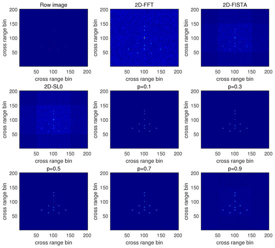
Figure 3. MIMO imaging results with 2D-FFT, 2D-FISTA, 2D-SL0, and the proposed algorithm with $p=0.1$, $p=0.3$, $p=0.5$, $p=0.7$, and $p=0.9$.

Table 2. Imaging performance.

Algorithm	2D-FFT	2D-FISTA	2D-SL0	p = 0.1	p = 0.3	p = 0.5	p = 0.7	p = 0.9
NMSE	4.048	2.0923	2.4894	0.4836	0.5100	0.5443	0.5629	0.8544
Corr	0.0450	0.1868	0.1703	0.8177	0.8025	0.7827	0.7788	0.6771

Both Figure 4 and Figure 5 illustrate the variation curve of the SNR with the NMSE and Corr, respectively, where the performance of the proposed algorithm is obviously better than the 2D-FFT, 2D-FISTA, and 2D-SL0 algorithms, especially under low SNRs. Meanwhile, the NMSE gradually decreases and the Corr ascends for all algorithms contained in Figure 4 and Figure 5, respectively, with the increase of the SNR. The result implies that the algorithm is more robust compared to the other algorithms. In our algorithm, we added the augmented Lagrange multiplier and $l_p$ penalty function to inhibit the outliers and improve the robustness of the algorithm.

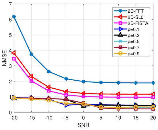
Figure 4. The relationship between the SNR and NMSE.

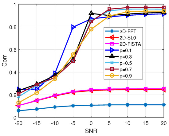
Figure 5. The relationship between the SNR and Corr.

Next, the influence of the percentage of outliers in the array on imaging performance was studied, and we set the percentage from $10\%$ to $60\%$. Their relationship can be seen in Figure 6 and Figure 7, which show that our algorithm is more robust than 2D-FISTA, 2D-SL0, and 2D-FISTA. The results also imply that the proposed algorithm is more robust to outliers.

Figure 6. The relationship between the percentage of outliers and the NMSE.

Figure 7. The relationship between the percentage of outliers and the Corr.

Public Dataset Experiment

Finally, we used a public dataset, the Boeing-727 dataset, to validate the performance of the proposed algorithm, which demonstrated that the dataset is consistent with the signal model for MIMO imaging. Suppose that every point in the radar echo matrix can be seen as the snapshot of the MIMO virtual array. The dataset is generated by an X-band (9.0 GHz) stepped frequency radar. The radar parameters are shown in the Table 3.

Table 3. The parameters of the step radar.

Parameters	Value
Center frequency	$9GHz$
Bandwidth	$150MHz$
Sampling points	64
Pulse number	256
SNR	$10dB$

In this experiment, we chose the number of transmitted frequencies and the number of weeps as 64 and 256, respectively, and the algorithm parameters were $p=0.1$, $\lambda =0.4$, $SNR=10dB$, and $P=1024,Q=256$. The radar imaging result can be seen in Figure 8 and Figure 9, whose percentage of outliers were set as $12\%$ and $39\%$, respectively. Our algorithm can well inhibit background noise and outliers compared to the existing algorithms.

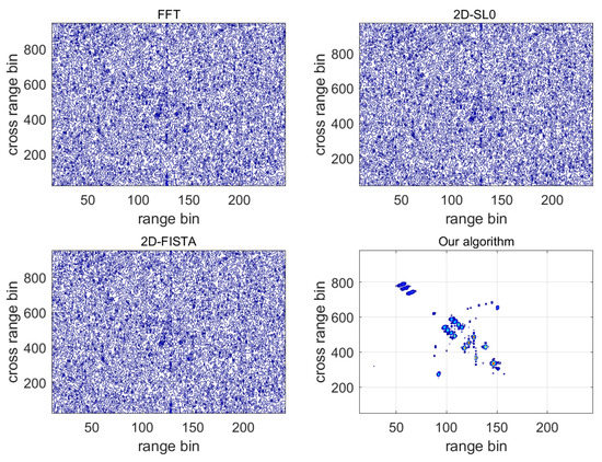
Figure 8. Imaging result with the percentage of outliers being $12\%$.

Figure 9. Imaging result with the the percentage of outliers being $39\%$.

5. Discussion

5.1. Algorithm Convergence Analysis

To evaluate the converge of both algorithms, the experiment conditions were $p=0.5$, $L=1\times {10}^6$, $\lambda =0.5$, and $SNR=10dB$. In Figure 10, although the exact algorithm can converge to a more concise result compared to the inexact algorithm, it can converge at a higher speed. The runtime and convergence error of both algorithms are presented in Table 4.

Figure 10. Convergence error curve of both algorithms.

Table 4. Runtime and convergence error of both algorithms.

Algorithm	Items	p = 0.1	p = 0.3	p = 0.5	p = 0.7
Exact recovery	Time (s)	179.1385	179.1395	179.1375	179.1363
	Error	0.0032	0.0041	0.0042	0.0042
Inexact recovery	Time (s)	3.3559	3.342	3.341	3.358
	Error	0.0088	0.0088	0.0086	0.0088

In Table 4, the result shows that the exact algorithm will speed up the time until the convergence condition is met, and the inexact recovery algorithm reduces the time complexity at the expense of the convergence accuracy.

5.2. Algorithm Complexity Analysis

On the one hand, we successfully recovered the uniform snapshot matrix from the contaminated snapshot matrix by the array outliers. On the other hand, the two algorithms, the exact recovery algorithm and the inexact recovery algorithm, were proposed to present the sparse imaging result, and $\mathbf{\Sigma }$ reflected the sparse position of the scattering points in space. In addition, the proposed algorithm was dominant in computational complexity.

Assume that the size of a contaminated snapshot matrix is $M\times N$, and the Fourier matrices are $M\times P$ and $N\times Q$. Generally, the computational complexity of SVD is around $\mathcal{O}\left(N{M}^2\right)+\mathcal{O}\left(M^3\right)$. The proposed algorithm in this paper was divided into three steps, and the computational complexity of every step can be seen below:

(1)

Updating $\mathbf{\Sigma }$: $\mathcal{O}\left(P^{2}M\right)+\mathcal{O}\left(P^{2}Q\right)+\mathcal{O}\left(Q^{2}N\right)$;

(2)

Updating $\mathbf{E}$: $\mathcal{O}\left(MPQ\right)+\mathcal{O}\left(MNQ\right)+\mathcal{O}\left(JPQ\right)$;

(3)

Updating $\mathbf{R}$: $\mathcal{O}\left(MPQ\right)+\mathcal{O}\left(MNQ\right)$.

For the exact recovery algorithm, the inner algorithm in Table 1 converges when it iterates K times. Thereby, the exact recovery algorithm will speed up the time more than the inexact recovery algorithm.

6. Conclusions

For MIMO radar 3D imaging, we achieved super-resolution imaging along the cross-range. The algorithm we proposed does not convert the grid matrix into the larger matrix and the observed matrix into the 1D vector and is more robust to noise than the existing algorithms, 2D-FISTA and 2D-SL0. We proposed two sparse recovery algorithms, the exact recovery algorithm and the inexact recovery algorithm, to inhibit the impact of outliers on the imaging performance. The simulation experiments and public dataset experiment validated the effectiveness of the algorithm.

References

- Ozdemir, C. Inverse Synthetic Aperture Radar Imaging with MATLAB Algorithms; Wiley: New York, NY, USA, 2012. [Google Scholar]
- Shakya, P.; Raj, A.B. Inverse Synthetic Aperture Radar Imaging Using Fourier Transform Technique. In Proceedings of the 2019 1st International Conference on Innovations in Information and Communication Technology (ICIICT), Chennai, India, 25–26 April 2019; pp. 1–4. [Google Scholar]
- Zhang, L.; Xing, M.; Qiu, C.W.; Li, J.; Sheng, J.; Li, Y.; Bao, Z. Resolution Enhancement for Inversed Synthetic Aperture Radar Imaging Under Low SNR via Improved Compressive Sensing. IEEE Trans. Geosci. Remote Sens. 2010, 48, 3824–3838. [Google Scholar] [CrossRef]
- Tian, B.; Lu, Z.; Liu, Y.; Li, X. Review on Interferometric ISAR 3D Imaging: Concept, Technology and Experiment. Signal Process. 2018, 153, 164–187. [Google Scholar] [CrossRef]
- Wang, D.W.; Ma, X.Y.; Chen, A.L.; Su, Y. High-resolution imaging using a wideband MIMO radar system with two distributed arrays. IEEE Trans. Image Process. 2009, 19, 1280–1289. [Google Scholar] [CrossRef]
- Bechter, J.; Roos, F.; Waldschmidt, C. Compensation of Motion-Induced Phase Errors in TDM MIMO Radars. IEEE Microw. Wirel. Components Lett. 2017, 27, 1164–1166. [Google Scholar] [CrossRef] [Green Version]
- Jian, L.; Stoica, P. MIMO Radar with Colocated Antennas. IEEE Signal Process. Mag. 2007, 24, 106–114. [Google Scholar]
- Miwa, T.; Ogiwara, S.; Yamakoshi, Y. MIMO Radar System for Respiratory Monitoring Using Tx and Rx Modulation with M-Sequence Codes. IEICE Trans. Commun. 2010, 93, 2416–2423. [Google Scholar] [CrossRef]
- Deng, H. Polyphase code design for Orthogonal Netted Radar systems. IEEE Trans. Signal Process. 2004, 52, 3126–3135. [Google Scholar] [CrossRef]
- Roberts, W.; Stoica, P.; Li, J.; Yardibi, T.; Sadjadi, F.A. Iterative Adaptive Approaches to MIMO Radar Imaging. IEEE Jour Sel. Top. Signal Process 2010, 4, 5–20. [Google Scholar] [CrossRef]
- Tan, X.; Roberts, W.; Li, J.; Stoica, P. Sparse Learning via Iterative Minimization with Application to MIMO Radar Imaging. IEEE Trans. Signal Process. 2011, 59, 1088–1101. [Google Scholar] [CrossRef]
- Ding, L.; Chen, W.; Zhang, W.; Poor, H.V. MIMO radar imaging with imperfect carrier synchronization: A point spread function analysis. IEEE Trans. Aerosp. Electron. Syst. 2015, 51, 2236–2247. [Google Scholar] [CrossRef]
- Ma, C.; Yeo, T.S.; Tan, C.S.; Liu, Z. Three-Dimensional Imaging of Targets Using Colocated MIMO Radar. IEEE Trans. Geosci. Remote Sens. 2011, 49, 3009–3021. [Google Scholar] [CrossRef]
- Zhu, Y.T.; Yi, S. A type of M 2-transmitter N 2-receiver MIMO radar array and 3D imaging theory. Sci. China 2011, 54, 2147–2157. [Google Scholar] [CrossRef]
- Hu, X.; Tong, N.; Zhang, Y.; Huang, D. MIMO Radar Imaging With Nonorthogonal Waveforms Based on Joint-Block Sparse Recovery. IEEE Trans. Geosci. Remote Sens. 2018, 56, 5985–5996. [Google Scholar] [CrossRef]
- Hu, X.; Tong, N.; Zhang, Y.; Wang, Y. 3D imaging using narrowband MIMO radar and ISAR technique. In Proceedings of the 2015 International Conference on Wireless Communications Signal Processing (WCSP), Nanjing, China, 15–17 October 2015; pp. 1–5. [Google Scholar] [CrossRef]
- Candes, E.J.; Wakin, M.B. An Introduction To Compressive Sampling. IEEE Signal Process. Mag. 2008, 25, 21–30. [Google Scholar] [CrossRef]
- Tropp, J.A.; Gilbert, A.C. Signal Recovery From Random Measurements Via Orthogonal Matching Pursuit. IEEE Trans. Inf. Theory 2007, 53, 4655–4666. [Google Scholar] [CrossRef] [Green Version]
- Babacan, S.D.; Molina, R.; Katsaggelos, A.K. Bayesian Compressive Sensing Using Laplace Priors. IEEE Trans. Image Process. 2010, 19, 53–63. [Google Scholar] [CrossRef]
- Beck, A.; Teboulle, M. A fast iterative shrinkage-thresholding algorithm for linear inverse problems. SIAM J. Imaging Sci. 2009, 2, 183–202. [Google Scholar] [CrossRef] [Green Version]
- Blumensath, T.; Davies, M.E. Iterative hard thresholding for compressed sensing. Appl. Comput. Harmon. Anal. 2009, 27, 265–274. [Google Scholar] [CrossRef] [Green Version]
- Wei, Z.; Zhang, B.; Xu, Z.; Han, B.; Hong, W.; Wu, Y. An Improved SAR Imaging Method Based on Nonconvex Regularization and Convex Optimization. IEEE Geosci. Remote Sens. Lett. 2019, 16, 1580–1584. [Google Scholar] [CrossRef]
- Xu, G.; Xing, M.; Zhang, L.; Liu, Y.; Li, Y. Bayesian Inverse Synthetic Aperture Radar Imaging. IEEE Geosci. Remote Sens. Lett. 2011, 8, 1150–1154. [Google Scholar] [CrossRef]
- Kang, H.; Li, J.; Guo, Q.; Martorella, M. Pattern Coupled Sparse Bayesian Learning Based on UTAMP for Robust High Resolution ISAR Imaging. IEEE Sens. J. 2020, 20, 13734–13742. [Google Scholar] [CrossRef]
- Ding, J.; Wang, M.; Kang, H.; Wang, Z. MIMO Radar Super-Resolution Imaging Based on Reconstruction of the Measurement Matrix of Compressed Sensing. IEEE Geosci. Remote Sens. Lett. 2022, 19, 1–5. [Google Scholar] [CrossRef]
- Ding, L.; Chen, W. MIMO Radar Sparse Imaging With Phase Mismatch. IEEE Geosci. Remote Sens. Lett. 2015, 12, 816–820. [Google Scholar] [CrossRef]
- Duarte, M.F.; Baraniuk, R.G. Kronecker compressive sensing. IEEE Trans. Image Process. 2011, 21, 494–504. [Google Scholar] [CrossRef]
- Ghaffari, A.; Babaie-Zadeh, M.; Jutten, C. Sparse decomposition of two dimensional signals. In Proceedings of the 2009 IEEE International Conference on Acoustics, Speech and Signal Processing, Taipei, Taiwan, 19–24 April 2009; pp. 3157–3160. [Google Scholar] [CrossRef] [Green Version]
- Wimalajeewa, T.; Eldar, Y.C.; Varshney, P.K. Recovery of sparse matrices via matrix sketching. arXiv 2013, arXiv:1311.2448. [Google Scholar]
- Liu, Z.; You, P.; Wei, X.; Li, X. Dynamic ISAR Imaging of Maneuvering Targets Based on Sequential SL0. IEEE Geosci. Remote Sens. Lett. 2013, 10, 1041–1045. [Google Scholar] [CrossRef]
- Jiang, X.; Yasotharan, A.; Kirubarajan, T. Robust Beamforming with Sidelobe Suppression for Impulsive Signals. IEEE Signal Process. Lett. 2015, 22, 346–350. [Google Scholar] [CrossRef]
- Wang, B.; Zhang, Y.D.; Wang, W. Robust DOA Estimation in the Presence of Miscalibrated Sensors. IEEE Signal Process. Lett. 2017, 24, 1073–1077. [Google Scholar] [CrossRef]
- Kou, J.; Li, M.; Jiang, C. Robust Direction-of-Arrival Estimation for Coprime Array in the Presence of Miscalibrated Sensors. IEEE Access 2020, 8, 27152–27162. [Google Scholar] [CrossRef]
- Kou, J.X.; Li, M.; Wang, L.; Yang, K.; Jiang, C.L. Generalized weight function selection criteria for the compressive sensing based robust DOA estimation methods. Signal Process. 2020, 175, 107663. [Google Scholar] [CrossRef]
- Rakotomamonjy, A.; Flamary, R.; Gasso, G. DC Proximal Newton for Nonconvex Optimization Problems. IEEE Trans. Neural Netw. Learn. Syst. 2016, 27, 636–647. [Google Scholar] [CrossRef] [PubMed] [Green Version]
- Candes, E.J.; Plan, Y. Matrix Completion With Noise. Proc. IEEE 2010, 98, 925–936. [Google Scholar] [CrossRef] [Green Version]
- Zeng, W.J.; So, H.C. Outlier-Robust Matrix Completion via ℓp-Minimization. IEEE Trans. Signal Process. 2018, 66, 1125–1140. [Google Scholar] [CrossRef]
- Zuo, W.; Meng, D.; Zhang, L.; Feng, X.; Zhang, D. A Generalized Iterated Shrinkage Algorithm for Non-convex Sparse Coding. In Proceedings of the 2013 IEEE International Conference on Computer Vision, Sydney, Australia, 1–8 December 2013; pp. 217–224. [Google Scholar] [CrossRef] [Green Version]
Publisher’s Note: MDPI stays neutral with regard to jurisdictional claims in published maps and institutional affiliations. |
© 2022 by the authors. Licensee MDPI, Basel, Switzerland. This article is an open access article distributed under the terms and conditions of the Creative Commons Attribution (CC BY) license (https://creativecommons.org/licenses/by/4.0/).