
A Robust Sparse Imaging Algorithm Using Joint MIMO Array Manifold and Array Channel Outliers


Abstract
:1. Introduction
2. Methods
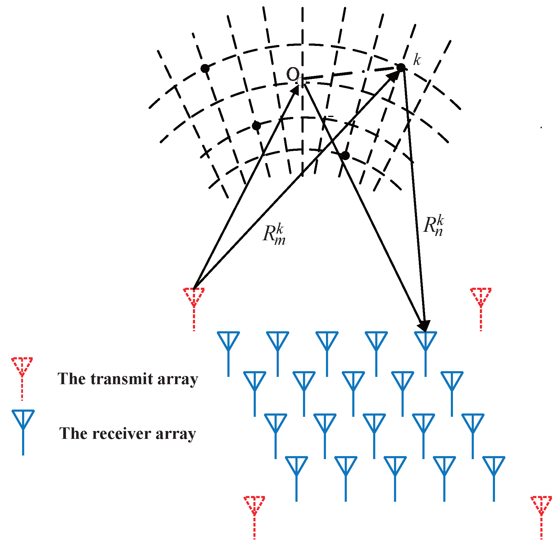
2.1. MIMO Imaging Model
2.2. The Composite Optimization
2.3. The Proposed Imaging Method
| Algorithm 1 Two-dimensional sparse solution of imaging results. |
Input:Convergence accuracy ; the maximum number of iterations K; Output: .
|
| Algorithm 2 Signal processing of CGISA. |
Input signal: , , p, J Output signal: .
|
| Algorithm 3 The exact sparse algorithm. |
Input: , , and Output: . |
| Algorithm 4 The inexact sparse algorithm. |
Input: , , and Output: . |
3. Results
4. Simulation Experiments
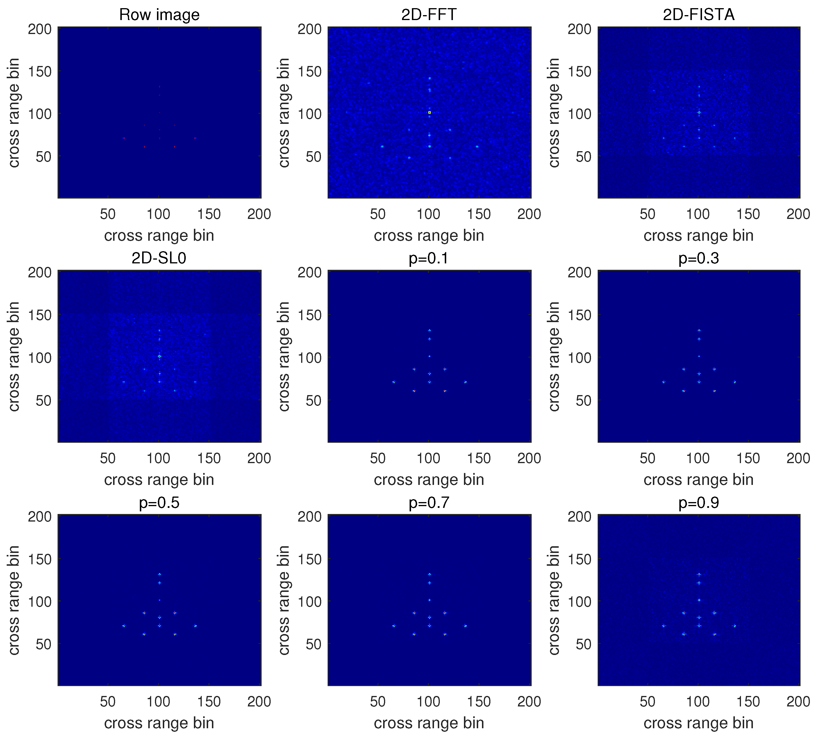
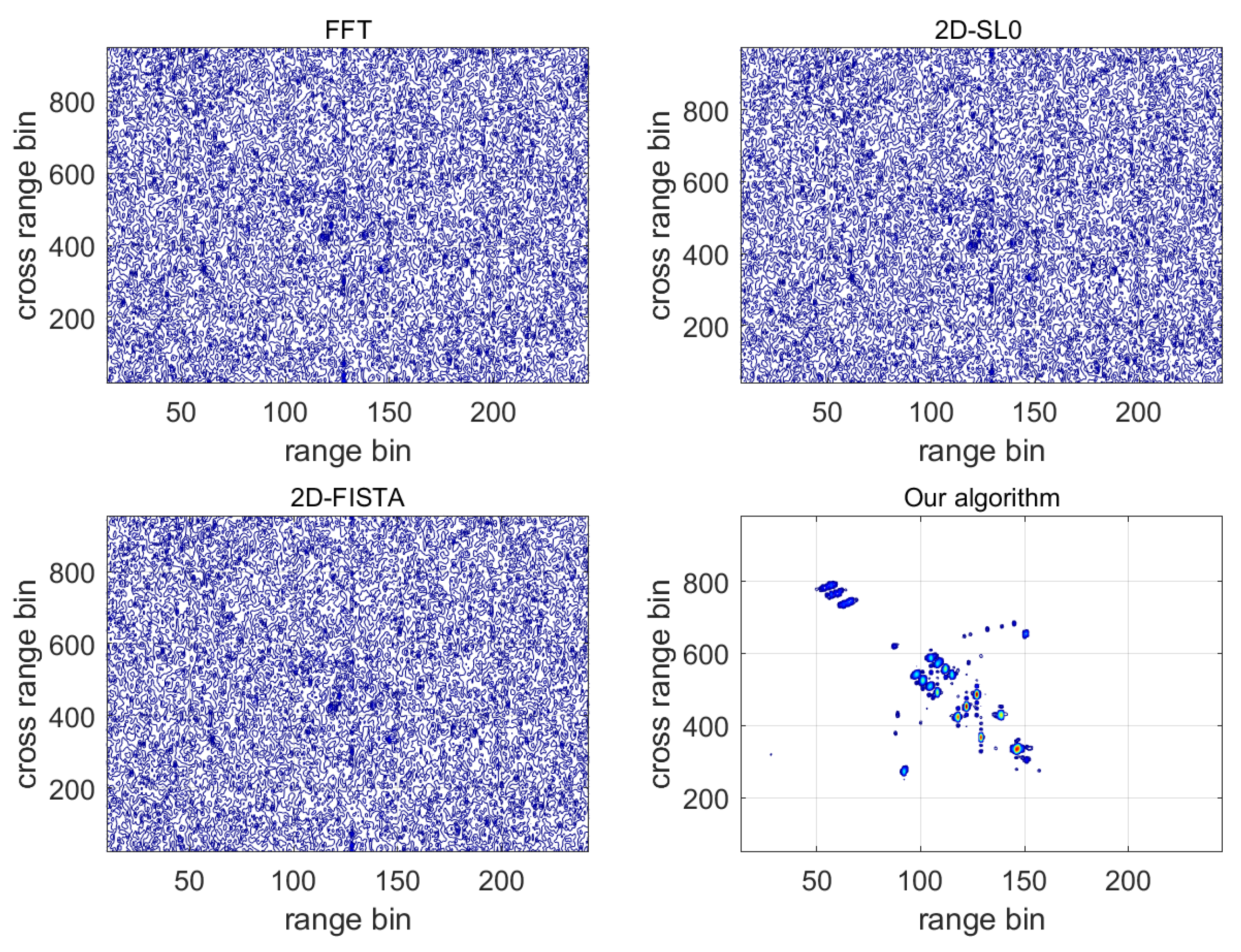
Public Dataset Experiment
5. Discussion
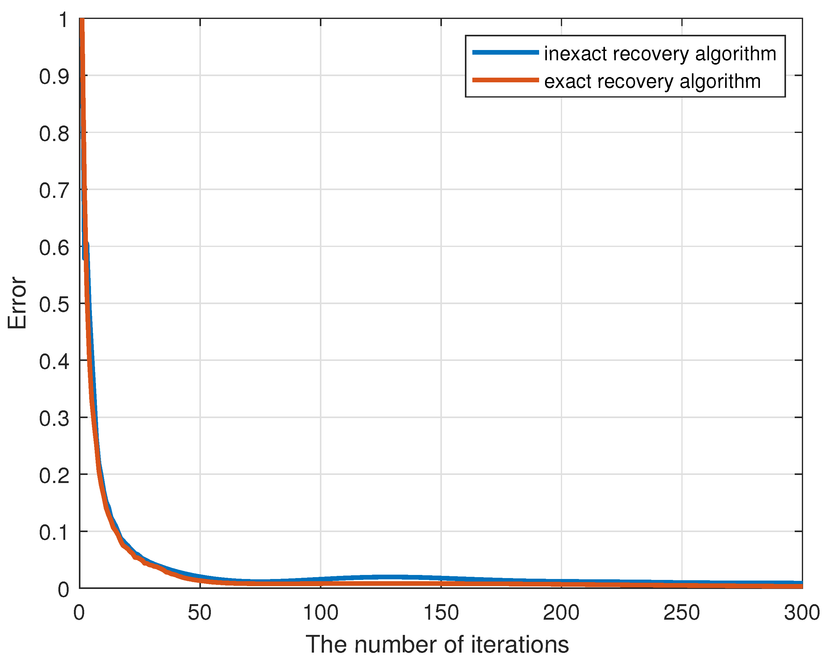
5.1. Algorithm Convergence Analysis
5.2. Algorithm Complexity Analysis
- (1)
- Updating : ;
- (2)
- Updating : ;
- (3)
- Updating : .
6. Conclusions
Author Contributions
Funding
Data Availability Statement
Acknowledgments
Conflicts of Interest
Abbreviations
| MIMO | multiple-input multiple-output |
| PAR | phased array radar |
| ADMM | alternative direction method of multipliers |
| ISAR | inverse synthetic aperture radar |
| SAR | synthetic aperture radar |
| MC | matrix completion |
| InISAR | interferometric ISAR |
| FDM | frequency-division multiplexing |
| TDM | time-division multiplexing |
| CDM | code-division multiplexing |
| PCA | phase center principle |
| BP | back projection |
| FRI | finite rate of innovation |
| SVT | singular-value thresholding |
| SBL | sparse Bayesian learning |
| GISA | generalized iterated shrinkage algorithm |
| CGISA | complex generalized iterated shrinkage algorithm |
| SL0 | smoothed L0 |
| ALM | augmented Lagrange multiplier method |
| SNR | signal-to-noise ratio |
| CS | compressive sensing |
| FFT | fast Fourier transform |
| FISTA | fast iterative shrinkage thresholding algorithm |
| SVD | singular-value decomposition |
| IALM | inexact augmented Lagrange multiplier |
| RAM | random access memory |
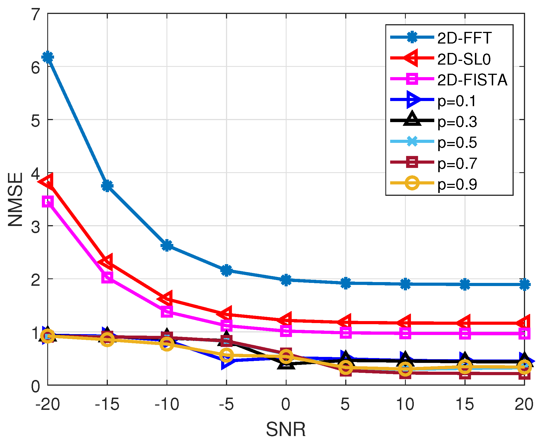
| NMSE | normal mean-squared error |
References
- Ozdemir, C. Inverse Synthetic Aperture Radar Imaging with MATLAB Algorithms; Wiley: New York, NY, USA, 2012. [Google Scholar]
- Shakya, P.; Raj, A.B. Inverse Synthetic Aperture Radar Imaging Using Fourier Transform Technique. In Proceedings of the 2019 1st International Conference on Innovations in Information and Communication Technology (ICIICT), Chennai, India, 25–26 April 2019; pp. 1–4. [Google Scholar]
- Zhang, L.; Xing, M.; Qiu, C.W.; Li, J.; Sheng, J.; Li, Y.; Bao, Z. Resolution Enhancement for Inversed Synthetic Aperture Radar Imaging Under Low SNR via Improved Compressive Sensing. IEEE Trans. Geosci. Remote Sens. 2010, 48, 3824–3838. [Google Scholar] [CrossRef]
- Tian, B.; Lu, Z.; Liu, Y.; Li, X. Review on Interferometric ISAR 3D Imaging: Concept, Technology and Experiment. Signal Process. 2018, 153, 164–187. [Google Scholar] [CrossRef]
- Wang, D.W.; Ma, X.Y.; Chen, A.L.; Su, Y. High-resolution imaging using a wideband MIMO radar system with two distributed arrays. IEEE Trans. Image Process. 2009, 19, 1280–1289. [Google Scholar] [CrossRef]
- Bechter, J.; Roos, F.; Waldschmidt, C. Compensation of Motion-Induced Phase Errors in TDM MIMO Radars. IEEE Microw. Wirel. Components Lett. 2017, 27, 1164–1166. [Google Scholar] [CrossRef] [Green Version]
- Jian, L.; Stoica, P. MIMO Radar with Colocated Antennas. IEEE Signal Process. Mag. 2007, 24, 106–114. [Google Scholar]
- Miwa, T.; Ogiwara, S.; Yamakoshi, Y. MIMO Radar System for Respiratory Monitoring Using Tx and Rx Modulation with M-Sequence Codes. IEICE Trans. Commun. 2010, 93, 2416–2423. [Google Scholar] [CrossRef]
- Deng, H. Polyphase code design for Orthogonal Netted Radar systems. IEEE Trans. Signal Process. 2004, 52, 3126–3135. [Google Scholar] [CrossRef]
- Roberts, W.; Stoica, P.; Li, J.; Yardibi, T.; Sadjadi, F.A. Iterative Adaptive Approaches to MIMO Radar Imaging. IEEE Jour Sel. Top. Signal Process 2010, 4, 5–20. [Google Scholar] [CrossRef]
- Tan, X.; Roberts, W.; Li, J.; Stoica, P. Sparse Learning via Iterative Minimization with Application to MIMO Radar Imaging. IEEE Trans. Signal Process. 2011, 59, 1088–1101. [Google Scholar] [CrossRef]
- Ding, L.; Chen, W.; Zhang, W.; Poor, H.V. MIMO radar imaging with imperfect carrier synchronization: A point spread function analysis. IEEE Trans. Aerosp. Electron. Syst. 2015, 51, 2236–2247. [Google Scholar] [CrossRef]
- Ma, C.; Yeo, T.S.; Tan, C.S.; Liu, Z. Three-Dimensional Imaging of Targets Using Colocated MIMO Radar. IEEE Trans. Geosci. Remote Sens. 2011, 49, 3009–3021. [Google Scholar] [CrossRef]
- Zhu, Y.T.; Yi, S. A type of M 2-transmitter N 2-receiver MIMO radar array and 3D imaging theory. Sci. China 2011, 54, 2147–2157. [Google Scholar] [CrossRef]
- Hu, X.; Tong, N.; Zhang, Y.; Huang, D. MIMO Radar Imaging With Nonorthogonal Waveforms Based on Joint-Block Sparse Recovery. IEEE Trans. Geosci. Remote Sens. 2018, 56, 5985–5996. [Google Scholar] [CrossRef]
- Hu, X.; Tong, N.; Zhang, Y.; Wang, Y. 3D imaging using narrowband MIMO radar and ISAR technique. In Proceedings of the 2015 International Conference on Wireless Communications Signal Processing (WCSP), Nanjing, China, 15–17 October 2015; pp. 1–5. [Google Scholar] [CrossRef]
- Candes, E.J.; Wakin, M.B. An Introduction To Compressive Sampling. IEEE Signal Process. Mag. 2008, 25, 21–30. [Google Scholar] [CrossRef]
- Tropp, J.A.; Gilbert, A.C. Signal Recovery From Random Measurements Via Orthogonal Matching Pursuit. IEEE Trans. Inf. Theory 2007, 53, 4655–4666. [Google Scholar] [CrossRef] [Green Version]
- Babacan, S.D.; Molina, R.; Katsaggelos, A.K. Bayesian Compressive Sensing Using Laplace Priors. IEEE Trans. Image Process. 2010, 19, 53–63. [Google Scholar] [CrossRef]
- Beck, A.; Teboulle, M. A fast iterative shrinkage-thresholding algorithm for linear inverse problems. SIAM J. Imaging Sci. 2009, 2, 183–202. [Google Scholar] [CrossRef] [Green Version]
- Blumensath, T.; Davies, M.E. Iterative hard thresholding for compressed sensing. Appl. Comput. Harmon. Anal. 2009, 27, 265–274. [Google Scholar] [CrossRef] [Green Version]
- Wei, Z.; Zhang, B.; Xu, Z.; Han, B.; Hong, W.; Wu, Y. An Improved SAR Imaging Method Based on Nonconvex Regularization and Convex Optimization. IEEE Geosci. Remote Sens. Lett. 2019, 16, 1580–1584. [Google Scholar] [CrossRef]
- Xu, G.; Xing, M.; Zhang, L.; Liu, Y.; Li, Y. Bayesian Inverse Synthetic Aperture Radar Imaging. IEEE Geosci. Remote Sens. Lett. 2011, 8, 1150–1154. [Google Scholar] [CrossRef]
- Kang, H.; Li, J.; Guo, Q.; Martorella, M. Pattern Coupled Sparse Bayesian Learning Based on UTAMP for Robust High Resolution ISAR Imaging. IEEE Sens. J. 2020, 20, 13734–13742. [Google Scholar] [CrossRef]
- Ding, J.; Wang, M.; Kang, H.; Wang, Z. MIMO Radar Super-Resolution Imaging Based on Reconstruction of the Measurement Matrix of Compressed Sensing. IEEE Geosci. Remote Sens. Lett. 2022, 19, 1–5. [Google Scholar] [CrossRef]
- Ding, L.; Chen, W. MIMO Radar Sparse Imaging With Phase Mismatch. IEEE Geosci. Remote Sens. Lett. 2015, 12, 816–820. [Google Scholar] [CrossRef]
- Duarte, M.F.; Baraniuk, R.G. Kronecker compressive sensing. IEEE Trans. Image Process. 2011, 21, 494–504. [Google Scholar] [CrossRef]
- Ghaffari, A.; Babaie-Zadeh, M.; Jutten, C. Sparse decomposition of two dimensional signals. In Proceedings of the 2009 IEEE International Conference on Acoustics, Speech and Signal Processing, Taipei, Taiwan, 19–24 April 2009; pp. 3157–3160. [Google Scholar] [CrossRef] [Green Version]
- Wimalajeewa, T.; Eldar, Y.C.; Varshney, P.K. Recovery of sparse matrices via matrix sketching. arXiv 2013, arXiv:1311.2448. [Google Scholar]
- Liu, Z.; You, P.; Wei, X.; Li, X. Dynamic ISAR Imaging of Maneuvering Targets Based on Sequential SL0. IEEE Geosci. Remote Sens. Lett. 2013, 10, 1041–1045. [Google Scholar] [CrossRef]
- Jiang, X.; Yasotharan, A.; Kirubarajan, T. Robust Beamforming with Sidelobe Suppression for Impulsive Signals. IEEE Signal Process. Lett. 2015, 22, 346–350. [Google Scholar] [CrossRef]
- Wang, B.; Zhang, Y.D.; Wang, W. Robust DOA Estimation in the Presence of Miscalibrated Sensors. IEEE Signal Process. Lett. 2017, 24, 1073–1077. [Google Scholar] [CrossRef]
- Kou, J.; Li, M.; Jiang, C. Robust Direction-of-Arrival Estimation for Coprime Array in the Presence of Miscalibrated Sensors. IEEE Access 2020, 8, 27152–27162. [Google Scholar] [CrossRef]
- Kou, J.X.; Li, M.; Wang, L.; Yang, K.; Jiang, C.L. Generalized weight function selection criteria for the compressive sensing based robust DOA estimation methods. Signal Process. 2020, 175, 107663. [Google Scholar] [CrossRef]
- Rakotomamonjy, A.; Flamary, R.; Gasso, G. DC Proximal Newton for Nonconvex Optimization Problems. IEEE Trans. Neural Netw. Learn. Syst. 2016, 27, 636–647. [Google Scholar] [CrossRef] [PubMed] [Green Version]
- Candes, E.J.; Plan, Y. Matrix Completion With Noise. Proc. IEEE 2010, 98, 925–936. [Google Scholar] [CrossRef] [Green Version]
- Zeng, W.J.; So, H.C. Outlier-Robust Matrix Completion via ℓp-Minimization. IEEE Trans. Signal Process. 2018, 66, 1125–1140. [Google Scholar] [CrossRef]
- Zuo, W.; Meng, D.; Zhang, L.; Feng, X.; Zhang, D. A Generalized Iterated Shrinkage Algorithm for Non-convex Sparse Coding. In Proceedings of the 2013 IEEE International Conference on Computer Vision, Sydney, Australia, 1–8 December 2013; pp. 217–224. [Google Scholar] [CrossRef] [Green Version]


| Parameters | Symbol | Value |
|---|---|---|
| Center frequency | ||
| Bandwidth | B | |
| Sampling frequency | ||
| The number of transmitters | ||
| The number of receivers |
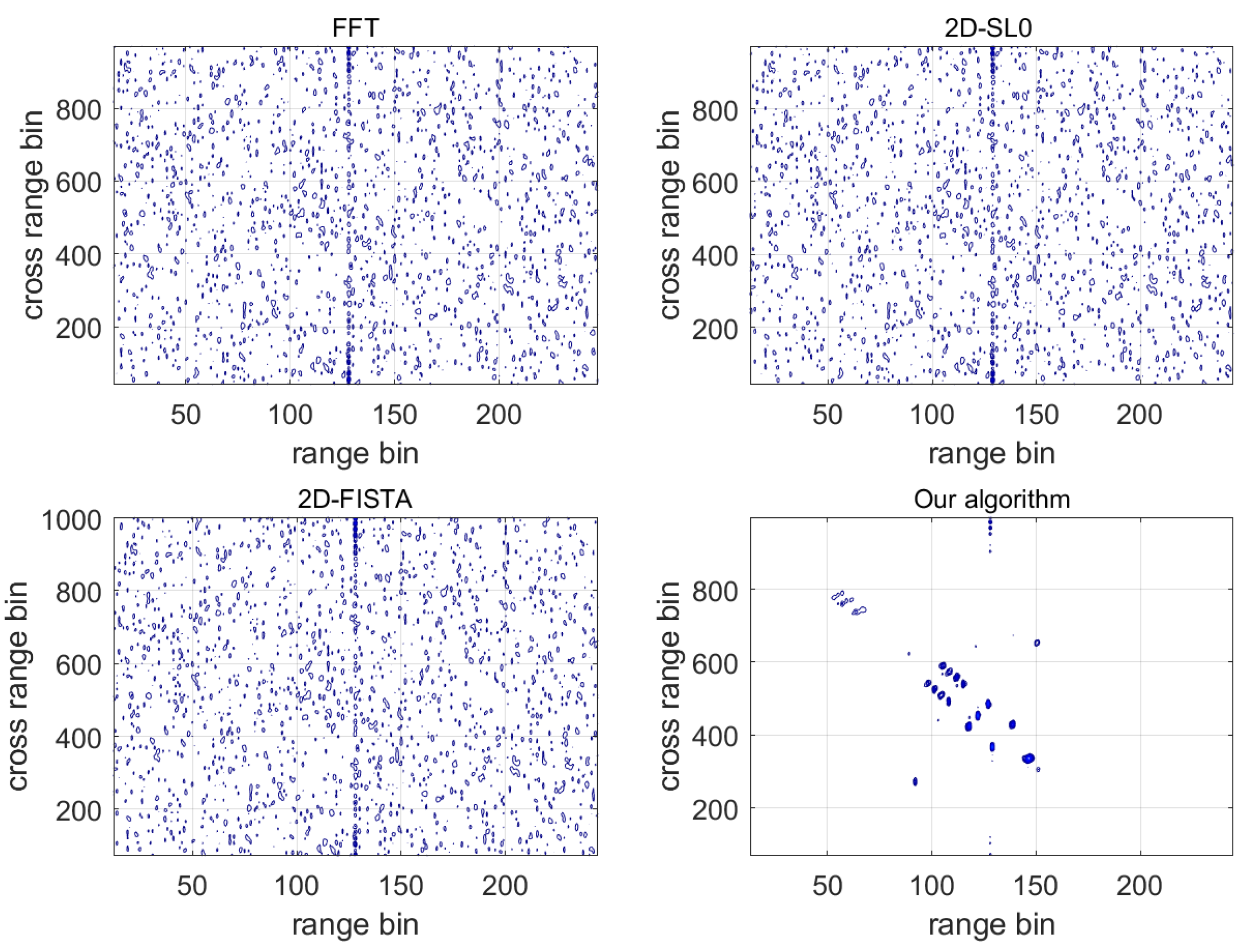
| Algorithm | 2D-FFT | 2D-FISTA | 2D-SL0 | p = 0.1 | p = 0.3 | p = 0.5 | p = 0.7 | p = 0.9 |
|---|---|---|---|---|---|---|---|---|
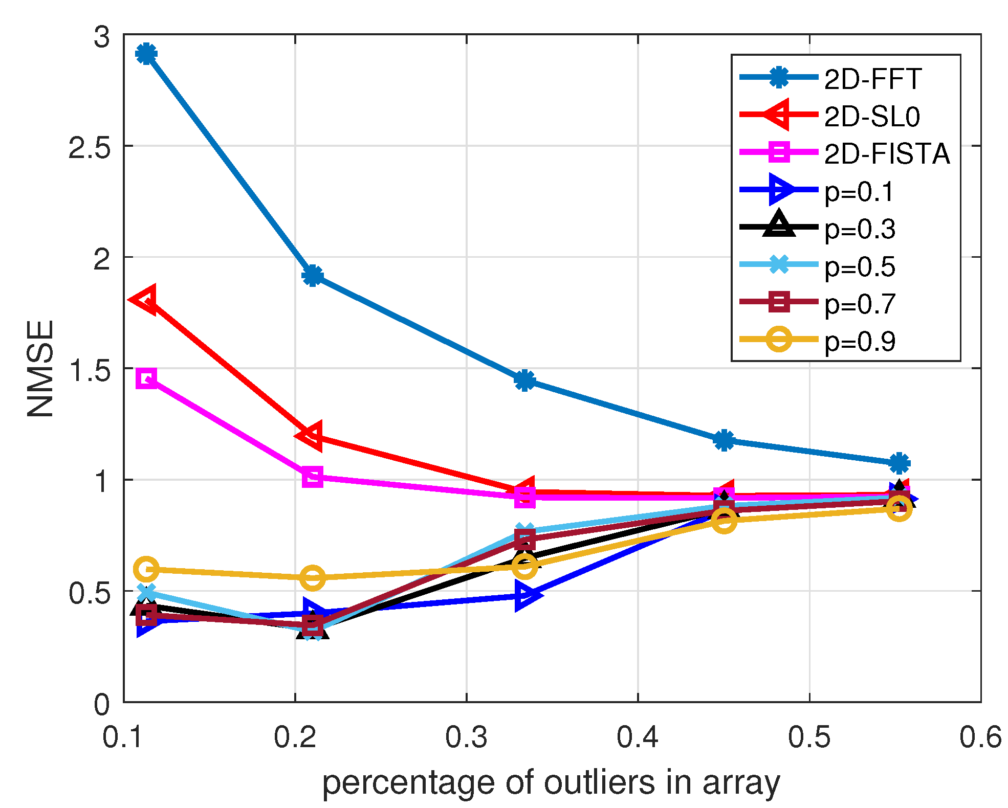
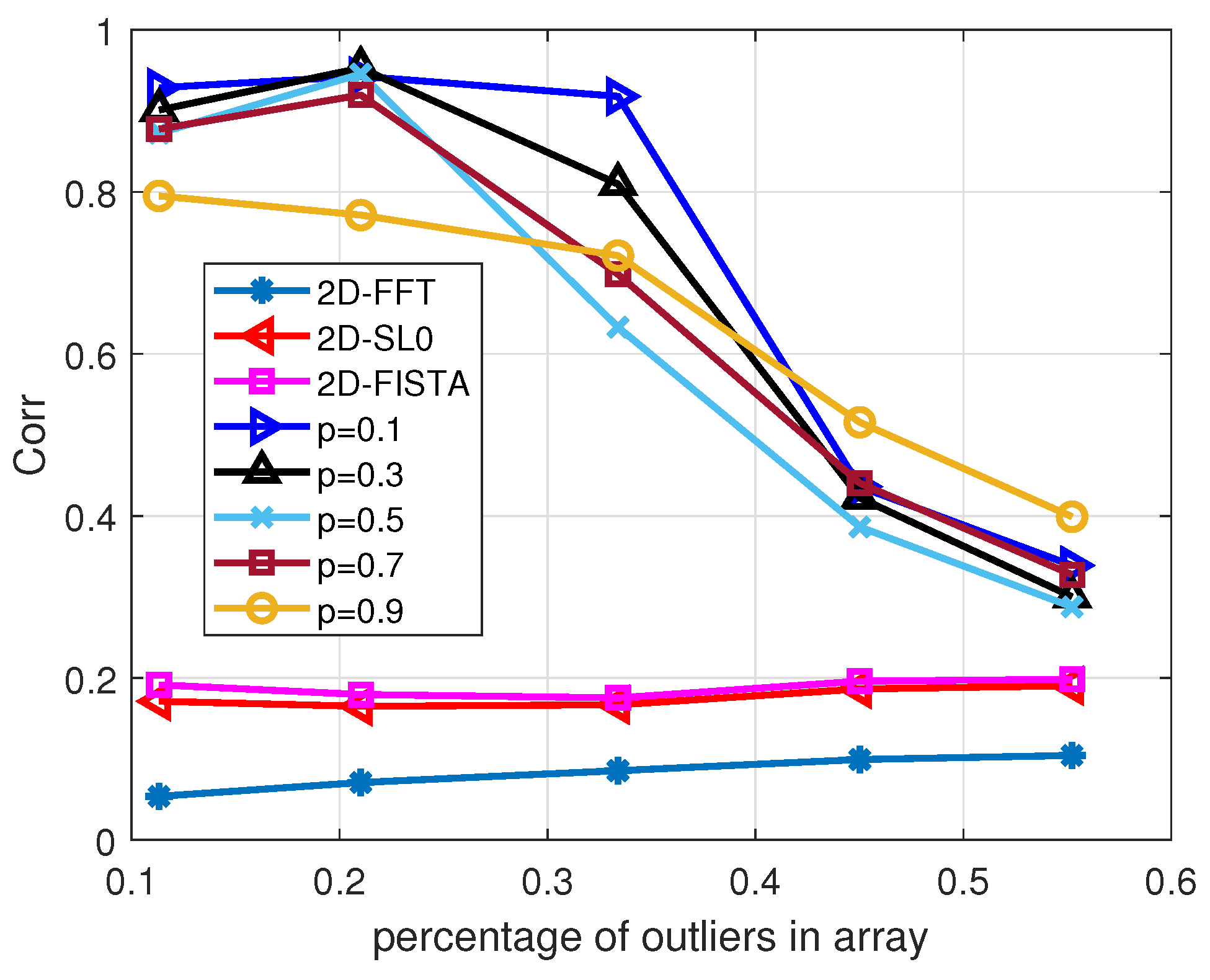
| NMSE | 4.048 | 2.0923 | 2.4894 | 0.4836 | 0.5100 | 0.5443 | 0.5629 | 0.8544 |
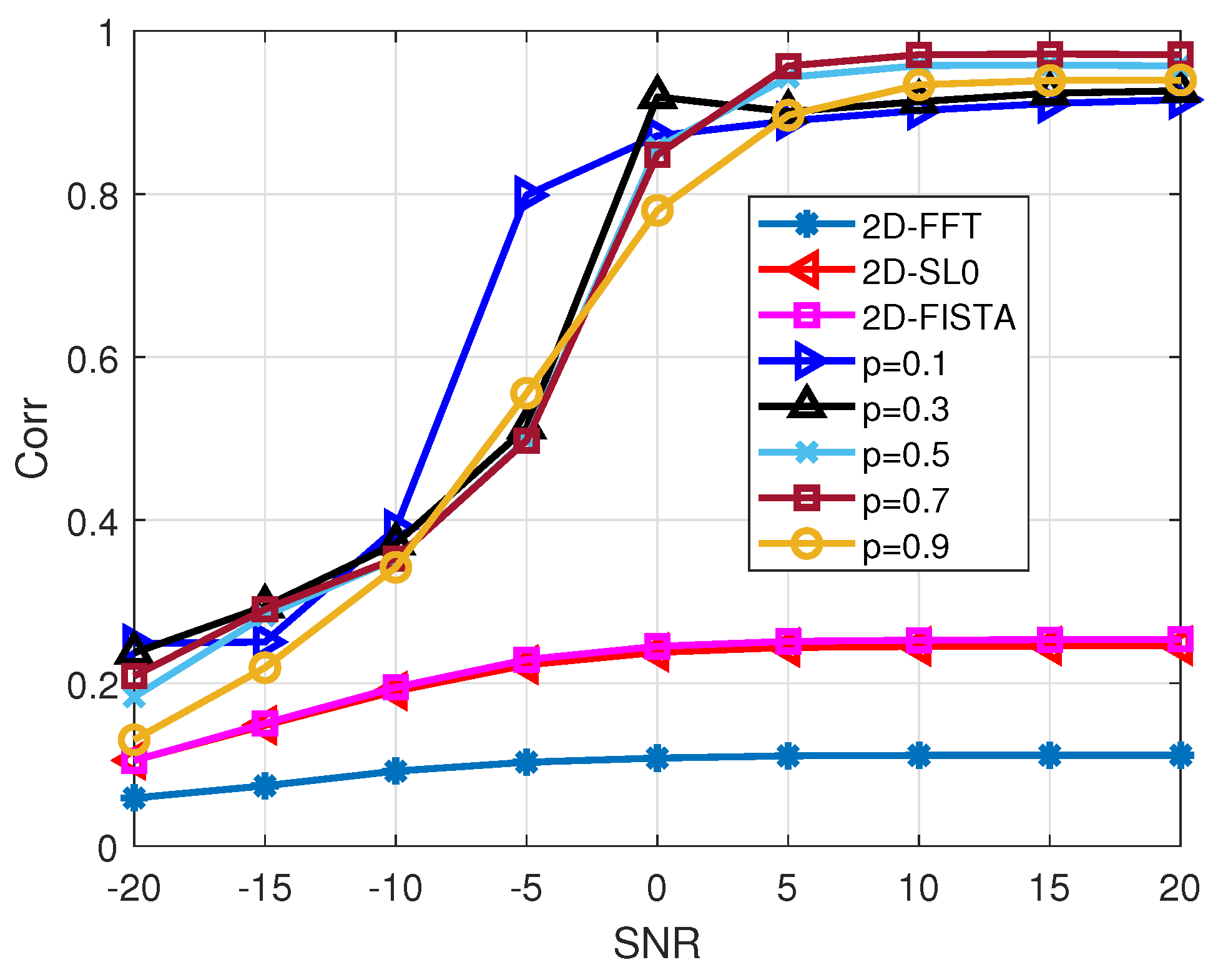
| Corr | 0.0450 | 0.1868 | 0.1703 | 0.8177 | 0.8025 | 0.7827 | 0.7788 | 0.6771 |
| Parameters | Value |
|---|---|
| Center frequency | |
| Bandwidth | |
| Sampling points | 64 |
| Pulse number | 256 |
| SNR |
| Algorithm | Items | p = 0.1 | p = 0.3 | p = 0.5 | p = 0.7 |
|---|---|---|---|---|---|
| Exact recovery | Time (s) | 179.1385 | 179.1395 | 179.1375 | 179.1363 |
| Error | 0.0032 | 0.0041 | 0.0042 | 0.0042 | |
| Inexact recovery | Time (s) | 3.3559 | 3.342 | 3.341 | 3.358 |
| Error | 0.0088 | 0.0088 | 0.0086 | 0.0088 |
Publisher’s Note: MDPI stays neutral with regard to jurisdictional claims in published maps and institutional affiliations. |
© 2022 by the authors. Licensee MDPI, Basel, Switzerland. This article is an open access article distributed under the terms and conditions of the Creative Commons Attribution (CC BY) license (https://creativecommons.org/licenses/by/4.0/).
Share and Cite
Ding, J.; Wang, Z.; Wu, X.; Wang, M. A Robust Sparse Imaging Algorithm Using Joint MIMO Array Manifold and Array Channel Outliers. Remote Sens. 2022, 14, 4120. https://doi.org/10.3390/rs14164120
Ding J, Wang Z, Wu X, Wang M. A Robust Sparse Imaging Algorithm Using Joint MIMO Array Manifold and Array Channel Outliers. Remote Sensing. 2022; 14(16):4120. https://doi.org/10.3390/rs14164120
Chicago/Turabian StyleDing, Jieru, Zhiyi Wang, Xinghui Wu, and Min Wang. 2022. "A Robust Sparse Imaging Algorithm Using Joint MIMO Array Manifold and Array Channel Outliers" Remote Sensing 14, no. 16: 4120. https://doi.org/10.3390/rs14164120
APA StyleDing, J., Wang, Z., Wu, X., & Wang, M. (2022). A Robust Sparse Imaging Algorithm Using Joint MIMO Array Manifold and Array Channel Outliers. Remote Sensing, 14(16), 4120. https://doi.org/10.3390/rs14164120