Abstract
Vegetation phenology not only describes the life cycle events of periodic plants during the growing season but also acts as an indicator of biological responses to climate change. Satellite monitoring of vegetation phenology can capture the spatial patterns of vegetation dynamics at global scales. However, the existing satellite products of global vegetation phenology still show uncertainties in estimating phenological metrices, especially for dormancy onset. The Second-Generation Global Imager (SGLI) onboard the satellite Global Change Observation Mission—Climate (GCOM-C) that launched in 2017 provides a new opportunity to improve the estimation of global vegetation phenology with a spatial resolution of 250 m. In this study, SGLI land surface reflectance data were employed to estimate the green-up and dormancy dates for different vegetation types based on a relative threshold method, in which a snow-free vegetation index (i.e., the normalized difference greenness index, NDGI) was adopted. The validation results show that there are significant agreements between the trajectories of the SGLI-based NDGI and the near-surface green color coordinate index (GCC) at the PhenoCam sites with different vegetation types. The SGLI-based estimation of the green-up dates slightly outperformed that of the existing MODIS and VIIRS phenology products, with an RMSE and R2 of 11.0 days and 0.71, respectively. In contrast, the estimation of the dormancy dates based on the SGLI data yielded much higher accuracies than the MODIS and VIIRS products, with an RMSE decreased from >23.8 days to 15.6 days, and R2 increased from <0.51 to 0.72. These results suggest that GCOM-C/SGLI data have the potential to generate improved monitoring of global vegetation phenology in the future.
1. Introduction
Vegetation phenology records certain seasonal events, such as germination, flowering, and falling leaves, and it is a highly sensitive indicator of terrestrial ecosystems’ response to long-term changes in climate [1,2,3]. The traditional method of collecting vegetation phenology is through in situ direct visual assessment, which has provided long-term records of specific phenological events for several decades [4,5]. To overcome the limitations of in situ observations (e.g., lack of consistency, continuity, and objectivity), remote sensing approaches have been proposed for phenology detection at local to global scales [6,7,8,9,10]. Over the past three decades, satellite-based studies of phenology have used coarse to moderate spatial resolution imagery from the Advanced Very High Resolution Radiometer (AVHRR), the MODerate resolution Imaging Spectroradiometer (MODIS), the Visible Infrared Imaging Radiometer Suite (VIIRS), and the Advanced Himawari Imager (AHI) [6,7,8,9,10,11,12]. The MODIS Global Land Cover Dynamics product (MCD12Q2) was operationally produced by NASA from time series of MODIS observations from 2000 to 2018 [13,14]. However, because the MODIS is nearing the end of its duty cycles, the VIIRS is intended to provide the operational standard to continue the MODIS records. The collection 1 VIIRS Global Land Surface Phenology (LSP) product (VNP22Q2) was released by NASA in late 2018 [10,15]. The MCD12Q2 and VNP22Q2 are the only global land surface phenology products currently available to the public. These products have been used to explore local and global phenological dynamics [16]. In addition to the MODIS and VIIRS phenology products, surface phenology estimated by medium- and high-resolution satellites, such as Landsat [17] and Sentinel-2 [18], and geosynchronous satellites, such as GOES [19] and Himawari-8 [12], has been discussed in many satellite-based surface phenology studies.
The current studies of satellite-based phenology, using optical remote sensing data, have developed a variety of different methods to extract phenological transition dates from the time series of vegetation indices [20,21], such as the normalized difference vegetation index (NDVI), the enhanced vegetation index (EVI) [7], the two-band enhanced vegetation index (EVI2), the plant phenology index (PPI) [22], and the normalized difference phenology index (NDPI) [23]. The NDVI and EVI2 are most used for characterizing vegetation dynamics from satellite data at local and global scales. However, both indices rise not only in response to vegetation greenness increasing in the spring phase but also in response to snowmelt, which may introduce uncertainty in phenology detection [24,25]. The novel developed vegetation index, the normalized difference greenness index (NDGI), was found to have improved performance in addressing the snowmelt effect on phenological detection [26]. Yang et al. [26] found that the potential of the NDGI for monitoring vegetation phenology was verified in tundra and grassland sites. In addition, the underlying idea of detecting the phenological transition dates from time series data is to use a function to fit the vegetation growth curve (i.e., asymmetric Gaussian, logistic, spline) and dates extracted by either a parameter inversion of the vegetation growth curve or a predefined threshold of the vegetation growth amplitude [7,13,14,27,28,29]. The parameter inversion method solves the inflection point of the vegetation growth curve from an approximately linear stage to another stage [7,10]. Usually, the maximum change rate in curvature is defined as the beginning or the end of vegetation growth. Unlike the parameter inversion method, the definition of the threshold method is more flexible [29]. The threshold can be set as needed to extract phenological indicators, for example, at 10% [21,30], 15% [14,21], 20% [8], 25% [31], or 50% [32].
It is challenging to evaluate satellite-retrieved phenology by in situ observation due to the limitations of the geographic scope of any given ground-based observation model [5,10]. Recently, the rapid development of near-surface phenological observation networks has provided monitoring of vegetation changes at the canopy to landscape scales. For example, the PhenoCam Network and the Phenological Eyes Network use a network camera installed at the top of the tower to automatically capture repeated images at high frequencies (several photos per day) [33,34]. Combining visual interpretation and image processing from these quantities of digital photos enables the phenology of the observed vegetation canopy to be characterized. The long-term records of these digital images have been proven to be a powerful tool for testing phenological indicators retrieved from satellites [12,21,35,36].
The Global Change Observation Mission—Climate (GCOM-C), carrying the optical sensor, the Second-Generation Global Imager (SGLI) with a 250 m spatial resolution and a 2–3 day revisit period, could provide the newest opportunity to monitor global vegetated surface since 2018 [37]. This paper presents a study aimed at generating and evaluating vegetation phenology estimated from 250 m SGLI NDGI data. To this end, the following questions are explored:
- (1)
- Are the observed seasonal trajectories of vegetation between the SGLI and near-surface consistent?
- (2)
- What is the agreement between the phenological transition dates derived from the SGLI and near-surface?
- (3)
- What is the difference in the spatial pattern of the phenological transition dates between the SGLI and the VIIRS?
2. Materials and Methods
2.1. SGLI Land Surface Reflectance and Vegetation Indices
The SGLI land surface reflectance product (RSRF) was retrieved from the top-of-atmosphere radiance (LTOA) with an algorithm developed mainly by the JAXA/Earth Observation Research Center (EORC) and obtained by integrating knowledge of atmospheric properties (aerosol scattering and absorption and radiative transfer models), land surface characteristics (spectral reflectance), and cloud and snow area detection [38]. We obtained the 250 m surface reflectance of SGLI band 3 (443 μm), band 5 (530 μm), band 8 (673.5 μm), and band 11 (868.5 μm) in 2018 in the northern hemisphere from the Globe Portal System by the Japanese Aerospace Exploration Agency (https://gportal.jaxa.jp/ (accessed on 16 June 2022)), and as the primary input to calculate vegetation indices. The SGLI RSRF product also provided quality assurance (QA) flags, including data lack, land/ocean, cloud, cloud shadow, snow/ice, etc. To maintain the simplicity of satellite data processing, we only processed cloud pixel masking without further processing snow contamination.
The NDGI was calculated using the SGLI cloud-free reflectance data to track seasonal variation in the land surface. The NDGI was developed by Yang et al. [26] and was shown to overcome the influence of phenology detection on snowmelt. The NDGI is calculated as follows:
where , and represent the reflectance from the green, red, and NIR bands of the SGLI, respectively. was determined to be 0.64 for the SGLI, which depends on the spectral configuration of a sensor (see Table S1 in Yang et al. [26]). Since the raw time series still needed to be smoothed to reduce noise, we used a moving three-window median to smooth abruptly changing outliers in the time series [39,40].
To define the land covers of the SGLI pixels, we used the MODIS 500 m land cover product (MCD12Q1) from 2018 to implement the phenology detection at the pixels with natural vegetation [41]. Note that we did not estimate the phenological transition dates at pixels with an artificial vegetation domain or indistinctive seasonal changes, including cropland, urban, permafrost, barren, and water bodies. The 500 m MODIS land cover data were resampled to a 250 m grid using the nearest neighbor method to match the spatial resolution of the SGLI RSRF data.
2.2. Detection of Phenological Transition Dates from Time Series
The logistic model was originally used to monitor crop growth in the scenario of field observation [42,43], and has been adopted to characterize vegetation growth patterns from remote sensing data [7,9,20]. Here, we used the double logistic model to fit the SGLI time series of each pixel. The double logistic model is expressed as follows:
where denotes the pixel value at the day of the year (DOY) , and are the maximum and background values during the year, respectively, and are the DOYs of the maximum slopes of the curve in the increasing and decreasing stages, and and are the slopes of the curve at DOYs and , respectively.
The six parameters used to describe the shape of the curve were determined by the least square method, which minimized the residual between Equation (2) and the time series of the vegetation index. We extracted 9 phenological transition dates (i.e., 10% to 50% of the threshold by 5% of the step) corresponding to the green-up and dormancy dates for each pixel in the rising and falling phases of vegetation greenness, respectively. Finally, we compared the near-surface phenological observations to determine the appropriate threshold.
2.3. Near-Surface Phenology Observation Data
The PhenoCam Network (PCN) was established in 2008 and mainly covers the United States and parts of Europe. The PCN has been established with over 600 sites to date in different ecosystems around the world, providing a record of vegetation change. In this study, we selected green-up and dormancy dates from 115 near-surface observation sites (Table S1). Sites that did not provide a record for 2018 and sites for which the corresponding satellite-scale phenology could not be estimated were removed. In all the selected sites, the dominant vegetation types included deciduous forest (DF: 64 sites, including 63 sites of broadleaf and 1 site of needleleaf), followed by grassland (GR: 24 sites), shrubs (SH: 14 sites), wetland (WL: 7 sites), and tundra (TN: 6 sites). The spatial distribution of the selected sites is shown in Figure 1.
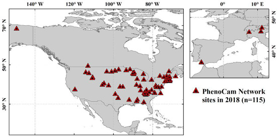
Figure 1.
Spatial distribution of near-surface phenology observation sites from PhenoCam Network.
The PhenoCam Network monitors the terrestrial ecosystem using digital repeat photography technology, which provides digital images every 30 min between 04:00–21:30 local time [44]. The data are stored on the PhenoCam server (https://phenocam.sr.unh.edu/ (accessed on 16 June 2022)) at the University of New Hampshire. Seyednasrollah et al. [44] generated the latest version of vegetation phenology datasets (version 2) from digital images during 2000–2018. The major two improvements of the version 2 dataset were that (1) the coverage was increased to 393 sites, and (2) the effect was corrected on the quality of the derived greenness time series due to the automatic white balancing. The PCN vegetation phenology dataset version 2 provided 6 phenological transition dates with 10%, 25%, and 50% of seasonal amplitude in the rising and falling phases at each site [33]. In this study, we used the green-up date (10% of amplitude in the rising phase) and dormancy date (10% of amplitude in the falling phase) from 115 sites in 2018.
2.4. MODIS and VIIRS Land Surface Phenology Products
In this study, we used satellite-based phenology data from the MCD12Q2 and VNP22Q2 products. The datasets were downloaded from the online Data Pool, courtesy of the NASA EOSDIS Land Processes Distributed Active Archive Center (LP DAAC) (https://lpdaa.usgs.gov/tools/data-pool/ (accessed on 16 June 2022)). Both products provide global land surface phenology with a 500 m spatial resolution and an annual step [14,45]. Phenological transition dates in the VNP22Q2 and MCD12Q2 are detected from the time series of the 2-band enhanced vegetation index (EVI2) using nadir bidirectional reflectance distribution function (BRDF)-adjusted reflectance (NBAR) data from the VIIRS and MODIS. However, the algorithms for detecting the transition dates in the MCD12Q2 and VNP22Q2 are different. Specifically, the MCD12Q2 uses penalized cubic splines to smooth the EVI2 time series and uses the thresholds of seasonal amplitude to determine (1) the green-up onset and dormancy onset (15% of amplitude), (2) mid-green-up and mid-senescence (50% of amplitude), and (3) maturity onset and senescence onset (90% of amplitude) [14]. The VNP22Q2 uses piecewise logistic functions to fit the EVI2 time series and uses the maxima of the rate of change in the curvature to determine the phenological transition dates, including (1) the onset of greenness increase, (2) the onset of the mid-green-up phase, (3) the onset of the greenness maximum, (4) the onset of greenness decrease, (5) the onset of the mid-senescence phase, and (6) the onset of the greenness minimum [10,45].
2.5. Evaluation of SGLI Phenology Using Near-Surface Phenology Observation
We tested a range of thresholds from 5% to 50% in steps of 5% to find the best thresholds for green-up and dormancy dates. We therefore initially assessed the agreement between 2 phenological transition dates from the SGLI and the near-surface observations. For each comparison, we computed the root mean square error (RMSE), standard deviation (SD), bias, coefficient of determination (R2), and statistical significance (p value). The bias was calculated relative to near-surface observations, so a positive bias indicates that the near-surface transition dates were earlier than the satellite-based transition dates. We randomly selected 70% of the sites (81 sites) from each vegetation type and, based on the results of the above comparison, chose a threshold value that minimized the uncertainty between the SGLI and the near-surface phenology observations. The remaining 30% of sites (34 sites) were used to verify whether the selected threshold was reasonable.
In addition, to illustrate the differences among satellite-based phenology, we also compared the phenological transition dates from the SGLI (our results), MODIS (MCD12Q2), and VIIRS (VNP22Q2) with those from the PCN at all 115 sites.
2.6. Comparison of SGLI Phenology with VIIRS Phenology
SGLI phenology was compared with VIIRS phenology to study the differences in the phenological transition dates between the two sensors. The VIIRS phenological detection method is briefly described in Section 2.4. As the MODIS duty cycle is coming to an end, the SGLI and VIIRS can replace the MODIS to continue to provide global surface vegetation observations. Therefore, it is also important to understand the agreement between the phenological transition dates retrieved from the SGLI and VIIRS. Here, we mainly compare the spatial distribution characteristics of the green-up and dormancy dates in the northern hemisphere of the SGLI and VIIRS and the differences between them.
3. Results
3.1. Time Series of SGLI and Near-Surface Observations and Determined Phenological Transition Dates
Figure 2 shows sample time series from raw satellite data and near-surface observations at five sites with different vegetation types (i.e., deciduous forest, grassland, shrub, tundra, and wetland). The raw time series of the NDGI and EIV2 derived from SGLI pixels show relatively large gaps and noises. The GCC time series derived from near-surface imagery exhibit more stable curves because of minimal atmospheric effects. At all sites, the coherence between the SGLI NDGI and the near-surface GCC is generally excellent, particularly in the greenness rising phase. It can be seen, however, that the GCC declined in autumn in advance of the NDGI. For the EVI2 time series, it started to increase earlier than the NDGI in spring, and the gradual decrease was slower than the NDGI in the green-up falling phase. In general, this shows that the SGLI NDGI can well characterize the seasonal changes in surface vegetation and is in good agreement with the near-surface observations. On the other hand, the NDGI did effectively suppress the effect of snow contamination. As can be seen in Figure 2a, the value of the EVI2 suddenly decreased from 0.4 to below 0.2 near day 50, while the NDGI was stable between 0.2 and 0.3. Using the photographs taken by the near-surface camera, we can see that snowfall caused a decrease in the EVI2 values (Figure S1).
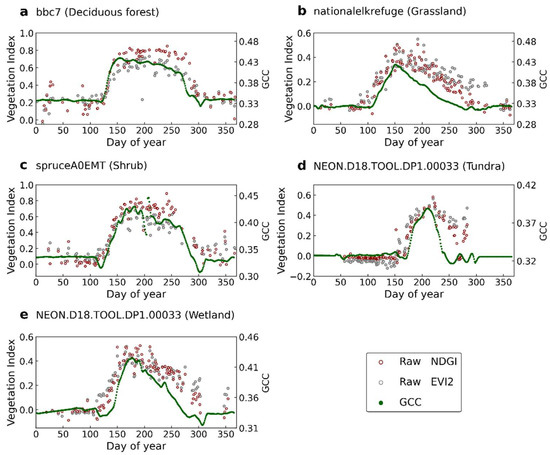
Figure 2.
The time series of the NDGI (red), EVI2 (gray), and GCC (green) at five locations with different vegetation types. Dots are raw observations from the SGLI. Green dots indicate the GCC obtained from near-surface observation data.
Table 1 shows a statistical summary that compares the green-up and dormancy dates from PCN observations at 81 sites against the SGLI based on different thresholds of the seasonal amplitude using a double logistic function. As the threshold continued to increase, the three statistical relationships gradually became smaller and then increased. By evaluating the consistency between the SGLI and the near-surface phenology observations, the 25% and 45% thresholds correspond to the green-up and dormancy dates for the PCN observations (Table 1 and Figure 3a,c) because they minimized the overall bias between the SGLI and the near-surface phenological transition dates. Using the determined thresholds, we also compared the SGLI and PCN phenology transition dates at the 34 sites used for validation (Figure 3b,d).

Table 1.
Statistical summaries for comparison between near-surface phenology and SGLI phenology using different thresholds for green-up date and dormancy date. The selected thresholds are shown in bold.
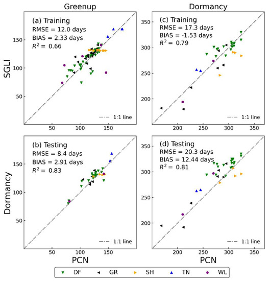
Figure 3.
Comparison of green-up and dormancy dates from SGLI and PCN observation by land cover types (DF: deciduous forest; GR: grassland, SH: shrub; TN: tundra; WL: wetland). (a,c) are comparisons at the 81 sites used to confirm the thresholds; (b,d) are comparisons at the 34 sites used to test the thresholds.
3.2. Comparison of Satellite Phenology with Near-Surface Phenology Observation
Figure 4 compares the satellite-based and near-surface-observed green-up and dormancy dates across the 115 PCN observation sites. Considering all the vegetation types, the green-up and dormancy dates estimated from the SGLI exhibited the best agreement with the near-surface observations, with RMSEs of 11–16 days, biases of less than 2.5 days, and R2 values higher than 0.71 (Figure 4a,b). By comparison, for the VIIRS and MODIS, the RMSEs ranged from 14 to 27 days, the average biases exceeded 9.9 days, and the R2 values ranged from 0.46 to 0.67 (Figure 4c–f). Overall, the correlations between the satellite and near-surface observations were consistently higher (the RMSE and bias were consistently lower) with the SGLI compared to the VIIRS and MODIS. The most notable improvement in agreement between the phenological transition dates from the SGLI and the near-surface observations relative to the VIIRS and MODIS was in the estimation of the dormancy dates.
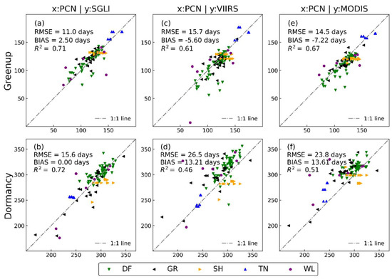
Figure 4.
Comparison of green-up and dormancy dates from satellite (SGLI (a,b), VIIRS (c,d), and MODIS (e,f)) and PCN observations by land cover types (DF: deciduous forest; GR: grassland, SH: shrub; TN: tundra; WL: wetland).
In the above analysis, we conflated all vegetation types and did not consider the differences between them. However, in the scatter plot in Figure 4, it is not difficult to see that the agreement between the satellite and near-surface observations is excellent for some vegetation. Table 2 summarizes the RMSE, bias, and R2 values by vegetation types between the green-up and dormancy dates estimated using satellite and near-surface observations. The agreement between the SGLI and near-surface for deciduous forest sites is less than five days. The RMSE of the SGLI is significantly smaller than those of the VIIRS and MODIS for both transition dates. However, the VIIRS and MODIS have a slightly better correlation with the near-surface for the dormancy date. For the grassland sites, the agreement between the SGLI and the near-surface is excellent. Unlike the deciduous forest sites, the differences in the RMSE and bias between the SGLI and near-surface are larger than those of the VIIRS and MODIS in the green-up dates for the grassland sites. However, the statistical results of the SGLI are superior to those of VIIRS and MODIS for the dormancy dates. For the shrub sites, poor coefficients of determination in both the green-up and dormancy dates indicate the relatively weak agreement between the satellite and near-surface observations. Note that all biases are negative, meaning that the green-up and dormancy dates obtained from the satellites in shrubs tend to be biased earlier than the near-surface observations. For the tundra sites, significant correlations (p < 0.1) were only found in the green-up dates from the MODIS and the dormancy dates from the SGLI and VIIRS. For the wetland sites, significant correlations (p < 0.1) were only found in the green-up dates from the VIIRS and the dormancy dates from the SGLI. Compared to the results of the other vegetation types, the RMSE of the wetlands is much higher. Indeed, it is apparent (Figure 4) that the agreement between the satellite and near-surface observations is much worse in the wetlands than in the other vegetation types. Note that there were not enough data for the tundra and wetland sites (n < 10 paired satellite-near-surface observations) to examine these patterns, which may be also a key factor contributing to these results.
Table 2.
Statistical comparison of green-up and dormancy dates from SGLI, VIIRS, and MODIS with those from near-surface phenology observations (PhenoCan network) in 115 sites by vegetation types (DF: deciduous forest; GR: grassland, SH: shrub; TN: tundra; WL: wetland). Green-up and dormancy dates from VIIRS and MODIS extracted from those phenology products (MCD12Q2 and VNP22Q2).
3.3. Spatial Distribution of SGLI Phenological Transition Dates
Compared to the observations at specific locations, the spatial distribution of the phenological transition dates can better explain the relationship between climate, land cover, and human activities. Figure 5 presents the spatial distribution of the green-up dates retrieved from the SGLI (Figure 5a) and the VIIRS (Figure 5b) and the relative differences (Figure 5c) in the northern hemisphere in 2018. However, in many arid and permafrost areas or areas with some vegetation and minimal seasonal changes, the phenology cannot be retrieved. Visual inspection shows that the spatial patterns are similar between the SGLI and the VIIRS for the green-up dates. The green-up dates for both satellites show a gradual delay across latitude, although these gradients could be interrupted. The relative differences in the retrieved green-up dates between the SGLI and VIIRS were relatively small in the high latitudes of the entire northern hemisphere. However, in the southeastern United States and temperate regions of Asia, the green-up dates of the SGLI were earlier than those of the VIIRS. These differences are concentrated to about 0 days with normal distribution between −50 and 50 days (Figure 5c), and the pixels with differences within ten days account for 58%.
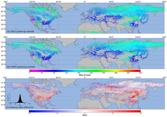
Figure 5.
Spatial distribution of green-up dates retrieved from SGLI (a) and VIIRS (b) and relative differences (c) in the northern hemisphere in 2018. Positive (negative) differences mean SGLI dates are later (earlier) than VIIRS dates.
Figure 6 shows the spatial distribution of the dormancy dates retrieved from the SGLI (Figure 6a) and the VIIRS (Figure 6b) and the relative differences (Figure 6c) in the northern hemisphere in 2018. Compared to the green-up dates, a gradual delay across latitudes for the SGLI dormancy dates is unclear. The earlier dormancy dates of the SGLI mainly occurred in Kazakhstan, Turkey, and the western United States, similar to the VIIRS. There are significant differences between the results of the SGLI and VIIRS on the dormant date in low latitudes. These differences also show a normal distribution between −50 days and 50 days, where differences of less than ten days account for approximately 34% of the total pixels, but the distribution slopes to the right (negative). Therefore, the dormancy dates of the SGLI were generally earlier than those of the VIIRS.
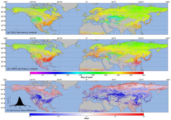
Figure 6.
Spatial distribution of dormancy dates retrieved from SGLI (a) and VIIRS (b) and relative difference (c) in the northern hemisphere in 2018. Positive (negative) differences mean SGLI dates are later (earlier) than VIIRS dates.
4. Discussion
Our analysis is the first to comprehensively evaluate the phenology estimation from the SGLI using a novel vegetation index, the NDGI, at the local to the hemispherical scale. At the pixel scale, the NDGI time series extracted from the SGLI can characterize the greenness trajectory of vegetation (Figure 2). Due to the NDGI being designed to address the snowmelt effect, we did not remove the snow-contaminated values using QA flags during pre-processing. However, while using NDVI or EVI2 phenology estimation, it is indispensable to use the QA flag or the normalized difference snow index to filter the snow data and use the background values to replace them [10,13,16,46]. Unreasonable background values will bring great uncertainty to detecting the phenological transition dates. The NDGI time series indeed presents the most similar pattern to the GCC compared to the NDVI and EIV2 between the SGLI and near-surface observations, especially during the rising period of greenness (Figure 7). In addition, the NDGI effectively restrained the snow noise in the ground background values. In a recent study by Cao et al. [25], the NDGI achieved much lower uncertainty in the detection of the green-up date than that of the NDVI. In addition, the NDGI changed more rapidly than the NDVI and EVI2 during the rapid growth or declining phase of vegetation (Figure 7). This is likely because the NDGI, similar to the GCC, is strongly sensitive to the greenness of the canopy, and it could be decreased with the color of green foliage fading in autumn. In contrast, the EVI2 is more sensitive to vegetation’s gross primary production and the fraction of photosynthetically active radiation. At the same time, the NDVI can better represent the change in the total leaf number of the vegetation canopy [22,26,47]. Consequently, it is not surprising that there are similar patterns in the greenness trajectories between the NDGI and the GCC.
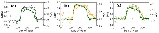
Figure 7.
Comparison of greenness trajectories from SGLI in different vegetation indices, including NDGI (a), NDVI (b), and EVI2 (c) with near-surface GCC.
In the analysis of the above threshold selection (Table 1), taking the green-up date as an example, the above results used the 25% threshold date as the SGLI data phenological indicator. However, for each vegetation type, different vegetation types may be suitable for different thresholds (Figure 8 and Figure S2). For example, for the deciduous forest sites (DF), although the correlation becomes slightly better as the threshold increases, the bias is less than one day at the 20% threshold. For the grass sites (GR), the bias is most minor for the 15% threshold, and the correlation is not particularly sensitive to this choice (R2 ≈ 0.57). For the shrub sites (SH), the agreement between the SGLI and near-surface is not significantly improved using any threshold. This can explain that in previous studies, the choice of different thresholds is crucial, especially when the dominant vegetation types are prevalent in the study region [29,30].
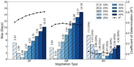
Figure 8.
Bias and coefficient of determination between green-up dates derived from SGLI and near-surface observation. Results are separated according to vegetation type (DF: deciduous forest; GR: grassland, SH: shrub). Progressively darker shades of blue designate green-up dates corresponding to different thresholds (10% to 50% of a threshold by 5% step).
The differences between the phenological transition dates from the SGLI NDGI and the near-surface GCC indicate that SGLI phenology is well detected in forests, followed by grasslands (Table 2). However, the phenological monitoring of shrubs, tundra, and wetlands is very complicated, possibly due to the spatial heterogeneity of the field of view between the SGLI and the near-surface camera [35,48,49]. Therefore, the phenological transition data from the SGLI and the near-surface observations are more comparable at homogeneous sites. To make more accurate evaluations using sensors with medium spatial resolution, high spatial–temporal resolution sensors can be used to match near-surface observations to footprints of medium spatial resolution.
Comparing the phenological transition dates from the SGLI, MODIS, and VIIRS with the near-surface phenological observations allowed us to understand the differences and similarities between the three sensors. Our results show that the agreement between the SGLI and near-surface phenology is the best (Figure 4), and the phenological transition dates estimated from the SGLI and VIIRS phenology products have similar spatial distributions (Figure 5 and Figure 6). The differences in the three satellite-based phenological estimations are due to several issues. First, the vegetation index used to generate the time series is inconsistent. Second, there are differences in the method of extracting the phenological transition dates from the raw time series. Xin et al. [30] indicated that the methods had significant differences in retrieving the phenological transition dates even using the same time series data. Third, the SGLI, with a spatial resolution of 250 m, is better than the MODIS and VIIRS. In recent years, phenology studies have begun using high-resolution imagery from Landsat-class and Sentinel-2 [31,48].
5. Conclusions
In this study, the GCOM-C/SGLI land surface reflectance product was applied to estimate the green-up and dormancy dates for different vegetation types based on a relative threshold method, in which a snow-free vegetation index (i.e., the normalized difference greenness index, NDGI) was adopted. Estimation accuracies were evaluated using the field measurements of the PhenoCam phenology network. The results show that there are significant agreements between the trajectories of the SGLI-based NDGI and the near-surface green color coordinate index (GCC) at the PhenoCam sites with different vegetation types. Regarding the estimation of the green-up dates, the SGLI data slightly outperformed the existing MODIS and VIIRS phenology products, with an RSME and R2 of 11.0 days and 0.71, respectively. In contrast, the SGLI-based estimation of the dormancy dates based on SGLI data yielded much higher accuracies than the MODIS and VIIRS products with an RSME decreased from >23.8 days to 15.6 days, and R2 increased from <0.51 to 0.72. These results suggest that the GCOM-C/SGLI data have the potential to generate improved monitoring of global vegetation phenology in the future.
Supplementary Materials
The following supporting information can be downloaded at: https://www.mdpi.com/article/10.3390/rs14164027/s1, Figure S1: Comparison of NDGI and EVI2 time series retrieved from SGLI (A). (B–D) are digital images from the PhenoCam Network site weather cameras corresponding to surface conditions at 27 days, 56 days, and 57 days, respectively; Figure S2: Bias and coefficient of determination between dormancy dates derived from SGLI and near-surface observation. Results are separated according to vegetation type (DF: deciduous forest; GR: grassland, SH: shrub). Progressively darker shades of red are used to designate dormancy dates corresponding to different thresholds (10% to 50% of threshold by 5% step); Table S1: Site characteristics of the PhenoCam Network and Phenology Eye Network sites used in this study. Vegetation types are as follows: DB = deciduous broadleaf; DN = deciduous needleleaf; GR = grassland; MX = mixed vegetation; SH = shrubs; TN = tundra; WL = wetland.
Author Contributions
Conceptualization, W.Y.; methodology, M.L. and W.Y.; project administration, W.Y.; supervision, W.Y.; writing—original draft, M.L.; writing—review and editing, M.L., W.Y. and A.K. All authors have read and agreed to the published version of the manuscript.
Funding
This research was funded by the JAXA Second Research Announcement on the Earth Observations (GCOM-C no. 106), the Japan Society for the Promotion of Science (JSPS) KAKENHI Grant (No. 20K12146), and the Japan Science and Technology Agency (JST) SPRING (grant number JPMJSP2109).
Acknowledgments
We thank our many collaborators, including the site PIs and technicians, for their efforts in support of PhenoCam. The development of PhenoCam has been funded by the Northeastern States Research Cooperative, NSF’s Macrosystems Biology program (awards EF-1065029 and EF-1702697), and DOE’s Regional and Global Climate Modeling program (award DE-SC0016011). We acknowledge the additional support from the US National Park Service Inventory and Monitoring Program and the USA National Phenology Network (grant number G10AP00129 from the United States Geological Survey), and from the USA National Phenology Network and North Central Climate Science Center (cooperative agreement number G16AC00224 from the United States Geological Survey). Additional funding, from the National Science Foundation’s LTER program, has supported research at Harvard Forest (DEB-1237491) and Bartlett Experimental Forest (DEB-1114804). We also thank the USDA Forest Service Air Resource Management program and the National Park Service Air Resources program for contributing their camera imagery to the PhenoCam archive.
Conflicts of Interest
The authors declare no conflict of interest.
References
- Badeck, F.W.; Bondeau, A.; Böttcher, K.; Doktor, D.; Lucht, W.; Schaber, J.; Sitch, S. Responses of Spring Phenology to Climate Change. New Phytol. 2004, 162, 295–309. [Google Scholar] [CrossRef]
- Peñuelas, J. Phenology Feedbacks on Climate Change. Science 2009, 324, 887–888. [Google Scholar] [CrossRef] [PubMed]
- Richardson, A.D.; Keenan, T.F.; Migliavacca, M.; Ryu, Y.; Sonnentag, O.; Toomey, M. Climate Change, Phenology, and Phenological Control of Vegetation Feedbacks to the Climate System. Agric. For. Meteorol. 2013, 169, 156–173. [Google Scholar] [CrossRef]
- Sparks, T.H.; Carey, P.D. The Responses of Species to Climate Over Two Centuries: An Analysis of the Marsham Phenological Record, 1736–1947. J. Ecol. 1995, 83, 321. [Google Scholar] [CrossRef]
- Richardson, A.D.; Bailey, A.S.; Denny, E.G.; Martin, C.W.; O’Keefe, J. Phenology of a Northern Hardwood Forest Canopy. Glob. Change Biol. 2006, 12, 1174–1188. [Google Scholar] [CrossRef]
- Reed, B.C.; Brown, J.F.; VanderZee, D.; Loveland, T.R.; Merchant, J.W.; Ohlen, D.O. Measuring Phenological Variability from Satellite Imagery. J. Veg. Sci. 1994, 5, 703–714. [Google Scholar] [CrossRef]
- Zhang, X.; Friedl, M.A.; Schaaf, C.B.; Strahler, A.H.; Hodges, J.C.F.; Gao, F.; Reed, B.C.; Huete, A. Monitoring Vegetation Phenology Using MODIS. Remote Sens. Environ. 2003, 84, 471–475. [Google Scholar] [CrossRef]
- White, M.A.; de Beurs, K.M.; Didan, K.; Inouye, D.W.; Richardson, A.D.; Jensen, O.P.; O’Keefe, J.; Zhang, G.; Nemani, R.R.; van Leeuwen, W.J.D.; et al. Intercomparison, Interpretation, and Assessment of Spring Phenology in North America Estimated from Remote Sensing for 1982–2006. Glob. Chang. Biol. 2009, 15, 2335–2359. [Google Scholar] [CrossRef]
- Busetto, L.; Colombo, R.; Migliavacca, M.; Cremonese, E.; Meroni, M.; Galvagno, M.; Rossini, M.; Siniscalco, C.; Morra Di Cella, U.; Pari, E. Remote Sensing of Larch Phenological Cycle and Analysis of Relationships with Climate in the Alpine Region. Glob. Chang. Biol. 2010, 16, 2504–2517. [Google Scholar] [CrossRef]
- Zhang, X.; Liu, L.; Liu, Y.; Jayavelu, S.; Wang, J.; Moon, M.; Henebry, G.M.; Friedl, M.A.; Schaaf, C.B. Generation and Evaluation of the VIIRS Land Surface Phenology Product. Remote Sens. Environ. 2018, 216, 212–229. [Google Scholar] [CrossRef]
- Tateishi, R.; Ebata, M. Analysis of Phenological Change Patterns Using 1982–2000 Advanced Very High Resolution Radiometer (AVHRR) Data. Int. J. Remote Sens. 2004, 25, 2287–2300. [Google Scholar] [CrossRef]
- Yan, D.; Zhang, X.; Nagai, S.; Yu, Y.; Akitsu, T.; Nasahara, K.N.; Ide, R.; Maeda, T. Evaluating Land Surface Phenology from the Advanced Himawari Imager Using Observations from MODIS and the Phenological Eyes Network. Int. J. Appl. Earth Obs. Geoinf. 2019, 79, 71–83. [Google Scholar] [CrossRef]
- Ganguly, S.; Friedl, M.A.; Tan, B.; Zhang, X.; Verma, M. Land Surface Phenology from MODIS: Characterization of the Collection 5 Global Land Cover Dynamics Product. Remote Sens. Environ. 2010, 114, 1805–1816. [Google Scholar] [CrossRef]
- Gray, J.; Sulla-Menashe, D.; Friedl, M.A. User Guide to Collection 6 MODIS Land Cover Dynamics (MCD12Q2) Product; NASA EOSDIS Land Processes DAAC: Missoula, MT, USA, 2019; Volume 6, pp. 1–8. Available online: https://modis-land.gsfc.nasa.gov/pdf/MCD12Q2_Collection6_UserGuide.pdf (accessed on 16 June 2022).
- Zhang, X.; Friedl, M.A.; Henebry, G.M. VIIRS Global Land Surface Phenology Product User Guide; United States Geological Survey: Reston, VA, USA, 2017; Volume 22. Available online: https://lpdaac.usgs.gov/documents/637/VNP22_User_Guide_V1.pdf (accessed on 16 June 2022).
- Zhang, X.; Liu, L.; Yan, D. Comparisons of Global Land Surface Seasonality and Phenology Derived from AVHRR, MODIS, and VIIRS Data. J. Geophys. Res. Biogeosci. 2017, 122, 1506–1525. [Google Scholar] [CrossRef]
- Li, L.; Li, X.; Asrar, G.; Zhou, Y.; Chen, M.; Zeng, Y.; Li, X.; Li, F.; Luo, M.; Sapkota, A.; et al. Detection and Attribution of Long-Term and Fine-Scale Changes in Spring Phenology over Urban Areas: A Case Study in New York State. Int. J. Appl. Earth Obs. Geoinf. 2022, 110, 102815. [Google Scholar] [CrossRef]
- Misra, G.; Cawkwell, F.; Wingler, A. Status of Phenological Research Using Sentinel-2 Data: A Review. Remote Sens. 2020, 12, 2760. [Google Scholar] [CrossRef]
- Wheeler, K.I.; Dietze, M.C. Improving the Monitoring of Deciduous Broadleaf Phenology Using the Geostationary Operational Environmental Satellite (GOES) 16 and 17. Biogeosciences 2021, 18, 1971–1985. [Google Scholar] [CrossRef]
- Xin, Q.; Li, J.; Li, Z.; Li, Y.; Zhou, X. Evaluations and Comparisons of Rule-Based and Machine-Learning-Based Methods to Retrieve Satellite-Based Vegetation Phenology Using MODIS and USA National Phenology Network Data. Int. J. Appl. Earth Obs. Geoinf. 2020, 93, 102189. [Google Scholar] [CrossRef]
- Stanimirova, R.; Cai, Z.; Melaas, E.K.; Gray, J.M.; Eklundh, L.; Jönsson, P.; Friedl, M.A. An Empirical Assessment of the MODIS Land Cover Dynamics and TIMESAT Land Surface Phenology Algorithms. Remote Sens. 2019, 11, 2201. [Google Scholar] [CrossRef]
- Jin, H.; Eklundh, L. A Physically Based Vegetation Index for Improved Monitoring of Plant Phenology. Remote Sens. Environ. 2014, 152, 512–525. [Google Scholar] [CrossRef]
- Wang, C.; Chen, J.; Wu, J.; Tang, Y.; Shi, P.; Black, T.A.; Zhu, K. A Snow-Free Vegetation Index for Improved Monitoring of Vegetation Spring Green-up Date in Deciduous Ecosystems. Remote Sens. Environ. 2017, 196, 1–12. [Google Scholar] [CrossRef]
- Delbart, N.; Kergoat, L.; le Toan, T.; Lhermitte, J.; Picard, G. Determination of Phenological Dates in Boreal Regions Using Normalized Difference Water Index. Remote Sens. Environ. 2005, 97, 26–38. [Google Scholar] [CrossRef]
- Cao, R.; Feng, Y.; Liu, X.; Shen, M.; Zhou, J. Uncertainty of Vegetation Green-up Date Estimated from Vegetation Indices Due to Snowmelt at Northern Middle and High Latitudes. Remote Sens. 2020, 12, 190. [Google Scholar] [CrossRef]
- Yang, W.; Kobayashi, H.; Wang, C.; Shen, M.; Chen, J.; Matsushita, B.; Tang, Y.; Kim, Y.; Bret-Harte, M.S.; Zona, D.; et al. A Semi-Analytical Snow-Free Vegetation Index for Improving Estimation of Plant Phenology in Tundra and Grassland Ecosystems. Remote Sens. Environ. 2019, 228, 31–44. [Google Scholar] [CrossRef]
- Sakamoto, T.; Yokozawa, M.; Toritani, H.; Shibayama, M.; Ishitsuka, N.; Ohno, H. A Crop Phenology Detection Method Using Time-Series MODIS Data. Remote Sens. Environ. 2005, 96, 366–374. [Google Scholar] [CrossRef]
- Jönsson, P.; Eklundh, L. Seasonality Extraction by Function Fitting to Time-Series of Satellite Sensor Data. IEEE Trans. Geosci. Remote Sens. 2002, 40, 1824–1832. [Google Scholar] [CrossRef]
- Shang, R.; Liu, R.; Xu, M.; Liu, Y.; Zuo, L.; Ge, Q. The Relationship between Threshold-Based and Inflexion-Based Approaches for Extraction of Land Surface Phenology. Remote Sens. Environ. 2017, 199, 167–170. [Google Scholar] [CrossRef]
- Huang, X.; Liu, J.; Zhu, W.; Atzberger, C.; Liu, Q. The Optimal Threshold and Vegetation Index Time Series for Retrieving Crop Phenology Based on a Modified Dynamic Threshold Method. Remote Sens. 2019, 11, 2725. [Google Scholar] [CrossRef]
- Tian, F.; Cai, Z.; Jin, H.; Hufkens, K.; Scheifinger, H.; Tagesson, T.; Smets, B.; van Hoolst, R.; Bonte, K.; Ivits, E.; et al. Calibrating Vegetation Phenology from Sentinel-2 Using Eddy Covariance, PhenoCam, and PEP725 Networks across Europe. Remote Sens. Environ. 2021, 260, 112456. [Google Scholar] [CrossRef]
- White, M.A.; Nemani, R.R. Real-Time Monitoring and Short-Term Forecasting of Land Surface Phenology. Remote Sens. Environ. 2006, 104, 43–49. [Google Scholar] [CrossRef]
- Richardson, A.D.; Hufkens, K.; Milliman, T.; Aubrecht, D.M.; Chen, M.; Gray, J.M.; Johnston, M.R.; Keenan, T.F.; Klosterman, S.T.; Kosmala, M.; et al. Tracking Vegetation Phenology across Diverse North American Biomes Using PhenoCam Imagery. Sci. Data 2018, 5, 180028. [Google Scholar] [CrossRef]
- Nasahara, K.N.; Nagai, S. Review: Development of an in Situ Observation Network for Terrestrial Ecological Remote Sensing: The Phenological Eyes Network (PEN). Ecol. Res. 2015, 30, 211–223. [Google Scholar] [CrossRef]
- Zhang, X.; Jayavelu, S.; Liu, L.; Friedl, M.A.; Henebry, G.M.; Liu, Y.; Schaaf, C.B.; Richardson, A.D.; Gray, J. Evaluation of Land Surface Phenology from VIIRS Data Using Time Series of PhenoCam Imagery. Agric. For. Meteorol. 2018, 256–257, 137–149. [Google Scholar] [CrossRef]
- Klosterman, S.T.; Hufkens, K.; Gray, J.M.; Melaas, E.; Sonnentag, O.; Lavine, I.; Mitchell, L.; Norman, R.; Friedl, M.A.; Richardson, A.D. Evaluating Remote Sensing of Deciduous Forest Phenology at Multiple Spatial Scales Using PhenoCam Imagery. Biogeosciences 2014, 11, 4305–4320. [Google Scholar] [CrossRef]
- Imaoka, K.; Kachi, M.; Fujii, H.; Murakami, H.; Hori, M.; Ono, A.; Igarashi, T.; Nakagawa, K.; Oki, T.; Honda, Y.; et al. Global Change Observation Mission (GCOM) for Monitoring Carbon, Water Cycles, and Climate Change. Proc. IEEE 2010, 98, 717–734. [Google Scholar] [CrossRef]
- Murakami, H. GCOM-C/SGLI Land Atmospheric Correction Algorithm; Japan Aerospace Exploration Agency: Tokyo, Japan, 2018; Volume 2018, pp. 1–12. Available online: https://suzaku.eorc.jaxa.jp/GCOM_C/data/ATBD/ver1/SGLI_Atmcorr_ATBD_v10.pdf (accessed on 16 June 2022).
- Ma, M.; Veroustraete, F. Reconstructing Pathfinder AVHRR Land NDVI Time-Series Data for the Northwest of China. Adv. Space Res. 2006, 37, 835–840. [Google Scholar] [CrossRef]
- Viovy, N.; Arino, O.; Belward, A.S. The Best Index Slope Extraction (BISE): A Method for Reducing Noise in NDVI Time-Series. Int. J. Remote Sens. 1992, 13, 1585–1590. [Google Scholar] [CrossRef]
- Friedl, M.A.; Sulla-Menashe, D.; Tan, B.; Schneider, A.; Ramankutty, N.; Sibley, A.; Huang, X. MODIS Collection 5 Global Land Cover: Algorithm Refinements and Characterization of New Datasets. Remote Sens. Environ. 2010, 114, 168–182. [Google Scholar] [CrossRef]
- Richards, F.J. A Flexible Growth Function for Empirical Use. J. Exp. Bot. 1959, 10, 290–301. [Google Scholar] [CrossRef]
- Yin, X.; Goudriaan, J.; Lantinga, E.A.; Vos, J.; Spiertz, H.J. A Flexible Sigmoid Function of Determinate Growth. Ann. Bot. 2003, 91, 361–371. [Google Scholar] [CrossRef]
- Seyednasrollah, B.; Young, A.M.; Hufkens, K.; Milliman, T.; Friedl, M.A.; Frolking, S.; Richardson, A.D. Tracking Vegetation Phenology across Diverse Biomes Using Version 2.0 of the PhenoCam Dataset. Sci. Data 2019, 6, 222. [Google Scholar] [CrossRef]
- Zhang, X.; Mark, A.; Friedl, G.M.H. VIIRS/NPP Land Cover Dynamics Yearly L3 Global 500m SIN Grid V001. Available online: https://lpdaac.usgs.gov/products/vnp22q2v001/ (accessed on 16 June 2022).
- Verger, A.; Filella, I.; Baret, F.; Peñuelas, J. Vegetation Baseline Phenology from Kilometric Global LAI Satellite Products. Remote Sens. Environ. 2016, 178, 1–14. [Google Scholar] [CrossRef]
- Fridley, J.D. Extended Leaf Phenology and the Autumn Niche in Deciduous Forest Invasions. Nature 2012, 485, 359–362. [Google Scholar] [CrossRef]
- Fisher, J.I.; Mustard, J.F.; Vadeboncoeur, M.A. Green Leaf Phenology at Landsat Resolution: Scaling from the Field to the Satellite. Remote Sens. Environ. 2006, 100, 265–279. [Google Scholar] [CrossRef]
- Richardson, A.D.; Hufkens, K.; Milliman, T.; Frolking, S. Intercomparison of Phenological Transition Dates Derived from the PhenoCam Dataset V1.0 and MODIS Satellite Remote Sensing. Sci. Rep. 2018, 8, 5679. [Google Scholar] [CrossRef]
Publisher’s Note: MDPI stays neutral with regard to jurisdictional claims in published maps and institutional affiliations. |
© 2022 by the authors. Licensee MDPI, Basel, Switzerland. This article is an open access article distributed under the terms and conditions of the Creative Commons Attribution (CC BY) license (https://creativecommons.org/licenses/by/4.0/).