Article

Thermal Contribution of the Local Climate Zone and Its Spatial Distribution Effect on Land Surface Temperature in Different Macroclimate Cities

1
School of Ecology and Environmental Sciences, Yunnan University, Kunming 650091, China
2
State Key Laboratory of Urban and Regional Ecology, Research Center for Eco-Environmental Sciences, Chinese Academy of Sciences, Beijing 100085, China
*
Author to whom correspondence should be addressed.
Remote Sens. 2022, 14(16), 4029; https://doi.org/10.3390/rs14164029
Submission received: 30 June 2022 / Revised: 15 August 2022 / Accepted: 16 August 2022 / Published: 18 August 2022
(This article belongs to the Special Issue Urban Planning Supported by Remote Sensing Technology)

Abstract

:
Local climate zones (LCZs) provide a comprehensive framework to examine surface urban heat islands (SUHIs), but information is lacking on their thermal contributions and spatial effects in different macroclimate cities. A standard framework for distinguishing between the cooling effect and heating effect and spatial effect analysis based on the LCZ scheme was conducted in five distinct macroclimate cities, i.e., Yuanjiang (arid climate), Jinghong (tropical climate), Kunming (subtropical climate), Zhaotong (temperate climate), and Shangri-La (alpine climate). The results indicated that (1) built-up zones presented heating effects in Jinghong and Shangri-La, but opposite results were observed in Yuanjiang and Zhaotong. (2) The thermal contributions of natural zones with dense trees (LCZAs) and waterbodies (LCZGs) showed cooling effects in the five cities regardless of season. (3) The spatial effect of heating LCZs on land surface temperature (LST) was more significant than that of cooling LCZs in Jinghong and Shangri-La, but the opposite results occurred in Yuanjiang and Kunming. Moreover, the spatial effect was lower in Zhaotong than in other cities. (4) Lower LST differences between natural zones and built-up zones in winter than in summer decreased the spatial effects. In summary, the thermal contributions of LCZs and their spatial heating/cooling effects were different among five distinct climate backgrounds, which implies that targeted measures must be used in different macroclimates.

1. Introduction

The global population increased from one billion people in 1800 to more than seven billion people in 2015 [1]. Rapid urbanization and global population increases have been accompanied by an increase in the intensity of landscape changes. This in turn has driven the development of urban heat islands (UHIs), which are defined as metropolitan areas with a higher temperature than that of surrounding areas [2]. UHIs notably affect the regional climate, vegetation growth, and water and air pollution, all of which are closely related to human health and the livability of cities [3,4,5]. Moreover, these negative impacts can be amplified by global warming [6]. Many studies have long remained interested in SUHI investigations because LST data can comprehensively cover entire cities [5].
The SUHI refers to the LST differences between different land uses and land covers (LULC) [7]. Different conditions across large areas can lead to different thermal characteristics, especially the macroclimate background. On the one hand, weather conditions alter the cooling effect of natural land cover by influencing evapotranspiration and vegetation conditions [8,9]. On the other hand, previous studies suggest that the relationship between LULC and LSTs exhibits spatial–temporal differences owing to climatic condition differentiation, which implies that the LSTs of built-up areas with various forms have different responses to macroclimate change [10,11,12]. Therefore, both artificial surfaces and natural land cover could present an opposite thermal contribution due to macroclimate differentiation and further contribute to different spatial effects [13].
In addition to the thermal contributions of different LULC types, previous studies have quantified the relationship between LSTs and landscape patterns. Studies on the spatial effects of heating/cooling LULC are crucial for urban planning and influencing mechanism analysis. Many landscape metrics concerning composition and configuration have shown large impacts on LSTs [14,15]. However, the correlation between LSTs and landscape patterns showed different results in some studies. For example, the density of the built-up areas had a positive correlation with LSTs [15,16], but a different result was shown in another study [16]. Furthermore, natural land cover had different spatial effects on LSTs in different cities [13]. Some studies suggest that seasonal and climate factors notably affect the relationship between urban landscapes and heat island effects [17,18]. For this reason, it is very important to determine the spatial effects of both heating and cooling LULC on LST variations in different macroclimate cities for better urban planning.
Many studies focus on the cooling effects of water bodies/green spaces and the heating effect of built-up areas [7,19,20], but the coupling of highly heterogeneous land with special physical properties and macroclimate backgrounds could lead to different thermal contributions and spatial effects, and it remains to be studied due to the lack of a uniform and comprehensive LULC classification scheme to quantify the thermal contributions and spatial effects. Inconsistencies in SUHI results among different studies pose a challenge in this field owing to the lack of a general LULC classification scheme reflecting the surface climate properties [21]. Thus, the concept of the local climate zone (LCZ) has been widely applied in urban climatology [22]. An LCZ is defined as a region with a uniform surface cover, structure, material, and human activities ranging in area from hundreds of meters to several kilometers on a horizontal scale [23,24]. Geometric and surface properties comprise the basis of LCZ classification. Therefore, this concept is more suitable for SUHI research than other frameworks, such as the national land cover database in the USA, the Urban Atlas, and the European CORINE land cover database [25]. Relevant studies have further revealed the relationship between LSTs and LCZs with different urban forms and surface properties [10,11,25,26,27,28,29]. However, few studies have systematically analyzed the thermal contributions of LCZs, and their spatial effects in different macroclimate cities are lacking [30,31].
The objectives of this study are thus to distinguish the cooling and heating effects of LCZs and investigate the relationship between the spatial distribution of heating/cooling LCZs and LST in five cities in Yunnan Province, China, with different background climates, namely, tropical, subtropical, temperate, alpine, and arid climates. Subsequently, the thermal distribution index (TDI) was used to quantify the magnitude of the heating/cooling contribution per LCZ. In addition, a thermal-weighted gravity index (TWGI) was proposed to reliably explain the LST variations. Particularly, the questions in this study are as follows: (1) Does the heating/cooling effect of LCZs differ among different macroclimate cities? (2) Should urban planners pay more attention to optimizing the spatial distribution of cooling LCZs or heating LCZs in different macroclimate cities?

2. Materials and Methods
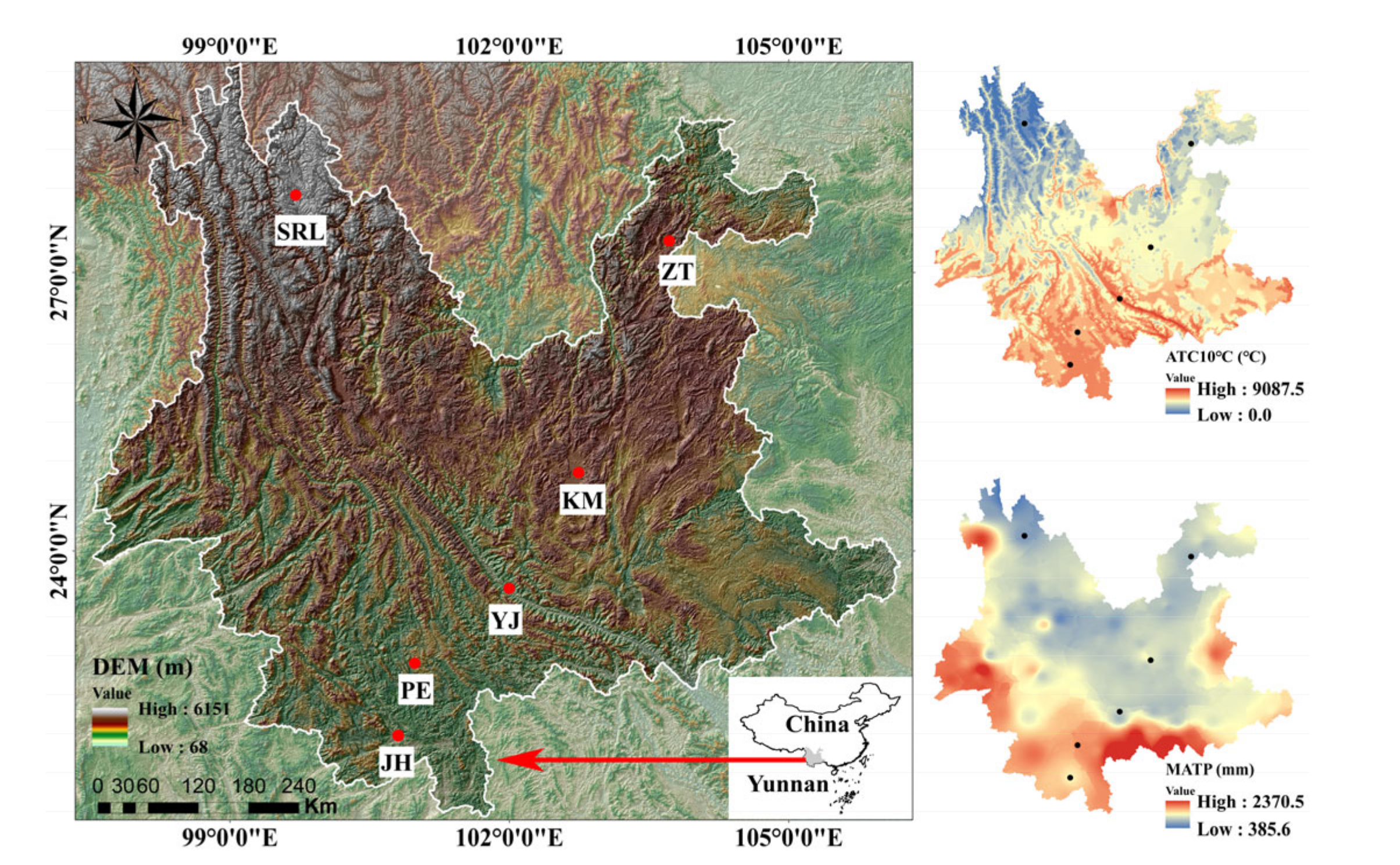
2.1. Study Area

Yunnan Province (21°09′–29°15′N and 97°32′–106°12′E), located in Southwest China, is a highland at a low latitude characterized by a highly heterogeneous terrain and fragile mountainous environment with a large difference in altitude, sharp changes in vertical topography, and a wide diversity of climate zones ranging from tropical to alpine zones [32]. A significant UHI phenomenon has been observed in Yunnan because of the rapid urbanization prompted by policies issued by the central government. Yunnan is divided into four climatic zones based on the number of days of the year with a temperature above 10 °C and an annual cumulative temperature above 10 °C (ATC10 °C), as obtained from China Green House Data (http://data.sheshiyuanyi.com/WeatherData/ (accessed on 19 May 2019)) [33]. Five cities were selected in this study. Jinghong is situated in a tropical area, Kunming and Zhaotong are cities in subtropical and temperate zones, respectively, and Shangri-La is located in an alpine climate zone (Figure 1). Yuanjiang was selected due to its arid climate. Table 1 lists data on the selected cities.

2.2. Methods

The overall research framework was divided into four steps in this study. First, reliable LCZ and LST maps were generated by using the modified World Urban Database and Access Portal Tool (WUDAPT) method and modified split-window algorithm, respectively. Second, the heating and cooling effects of each LCZ were differentiated by the threshold of the TDI value. Third, the spatial distribution of the heating/cooling LCZ was quantified by TWGI. Finally, ordinary least squares (OLS) and spatial regression were used to determine whether the spatial distribution of the heating/cooling LCZ has an impact on LST.

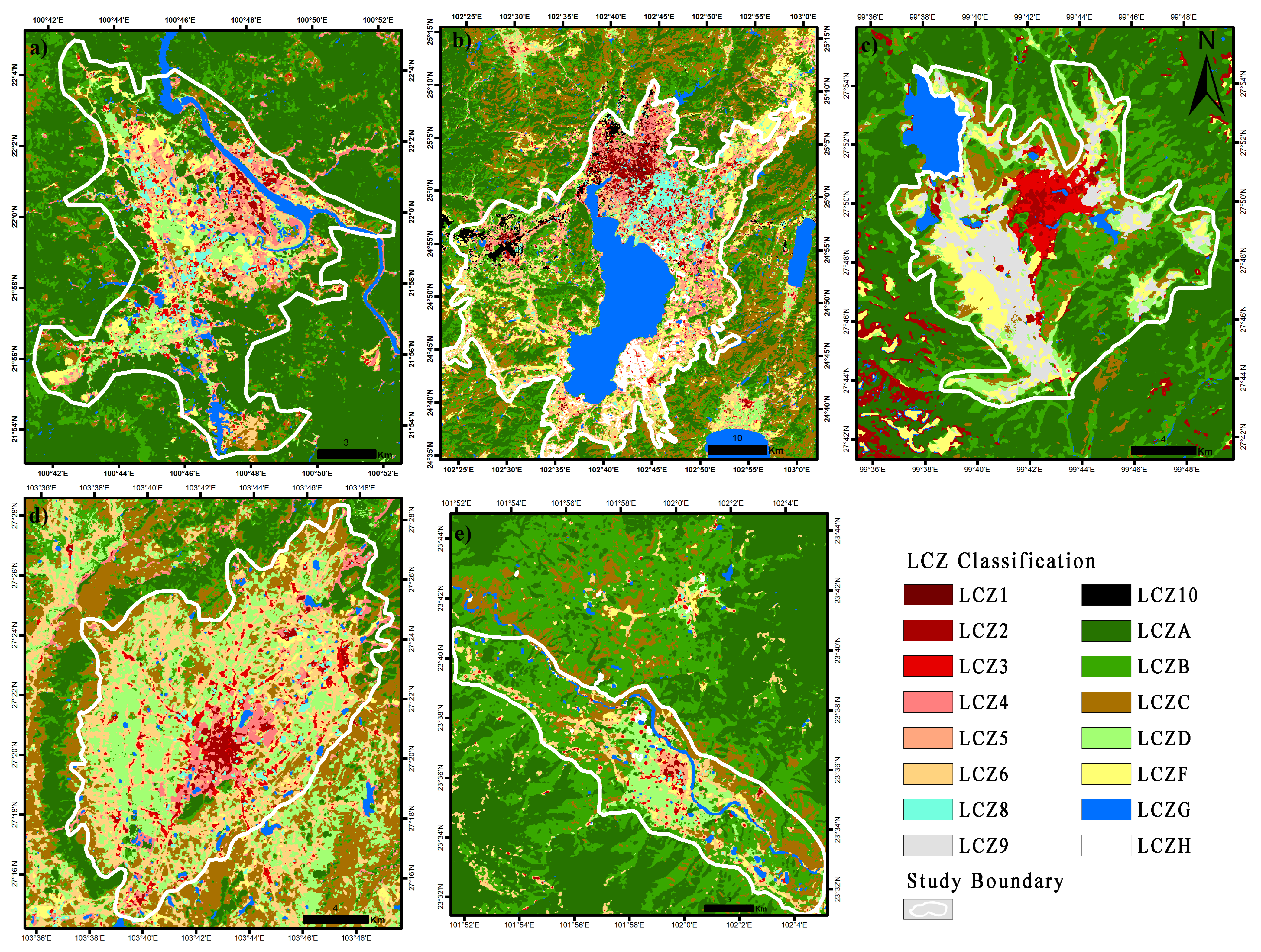
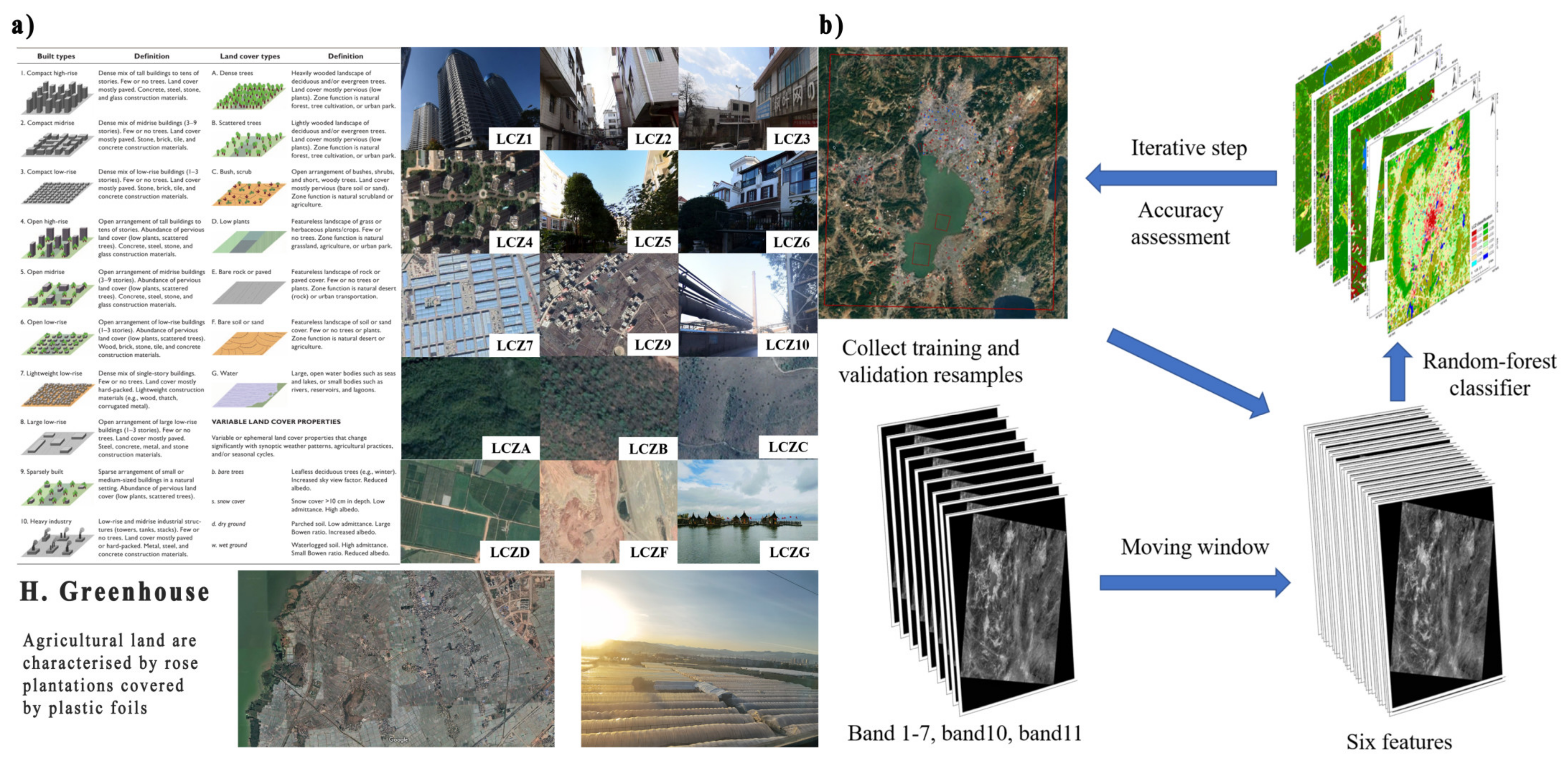
2.2.1. Map LCZ and LST

To study the LST difference among the five cities with different climatic backgrounds, Landsat 8 Operational Land Imager (OLI)/Thermal Infrared Sensor (TIRS) C1 Level-1 images were downloaded from the United States Geological Survey website (https://earthexplorer.usgs.gov/ (accessed on 12 October 2021)). Images featuring a cloud cover lower than 10% were selected for radiometric calibration and fast line-of-sight atmospheric analysis of spectral hypercubes (FLAASH) atmospheric correction in ENVI software. Images in summer and winter were selected in May and December, respectively, for LST retrieval in most cities except Shangri-La, where August and January are the hottest and coldest months, respectively (Table A1).
The workflow of LCZ mapping is shown in Figure 2. Seventeen standard LCZs were divided into 10 built-up type zones and seven land cover type zones. An extra natural LCZ, Greenhouse (LCZH), was defined due to its thermal response uncertainty. Owing to internal differentiation and horizontal heterogeneity in urban environments, especially in many rapidly developing cities of Yunnan, different LCZs mingle together on small surface areas, which degrades the quality of LCZ maps. The moving window method, which complies with the workflow of the WUDAPT, was used to capture information on neighborhoods for more accurate LCZ mapping [34]. Step 1 of the workflow involved the definition of the urban domain to be examined and the selection of training polygons for the different LCZs on Google Earth. To ensure the authenticity of the training data, the initial samples were selected based on field investigations and street-view Baidu Map images (https://map.baidu.com/ (accessed on 15 October 2021)). At least 10 representative samples were selected for the different LCZs in each city. Finally, 1768 training polygons and 732 evaluation polygons were collected. In Step 2, a contextual classifier was applied through the moving window method to obtain information. Six features (maximum, minimum, median, mean, and 25th and 75th quantile values) were calculated from all pixels within the moving windows of the predefined kernel size in Python 3.8. In Step 3, random forest classification was conducted in ENVI software. In Step 4, an accuracy assessment was conducted, and appropriate kernel sizes were used to map the LCZ for each city.
LST estimation was conducted based on a split-window algorithm, which can be expressed as Equation (1):
L S T = a 0 + a 1 + a 2 1 ε ε + a 3 Δ ε ε 2 T i + T j 2 + a 4 + a 5 1 ε ε + a 6 Δ ε ε 2 T i + T j 2 + a 7 T i T j 2
where a n (n = 0–7) is the algorithm coefficient; T i and T j are the brightness temperatures from the top of the atmosphere in bands 10 and 11, respectively; and ε and Δ ε are the emissivity mean and difference of the two channels, respectively.
The a n coefficient in Equation (1) was calculated in different atmospheric column water vapor (CWV) subranges [36]. The CWV was calculated with a modified split-window covariance–variance ratio method [37]. The land surface emissivity ( ε ) was calculated based on the normalized difference vegetation index (NDVI) as follows:
N D V I = N I R R N I R + R
F V C = N D V I N D V I s N D V I v N D V I s
ε = ε v · F V C + ε s 1 F V C + 4 d ε · F V C · 1 F V C
where NIR and R are the reflectance values of the near-infrared band and the red band, respectively; FVC is the fraction of vegetation cover; d ε is an effective value of the cavity effect of emissivity; and ε v and ε s are the vegetation and soil emissivity, respectively.

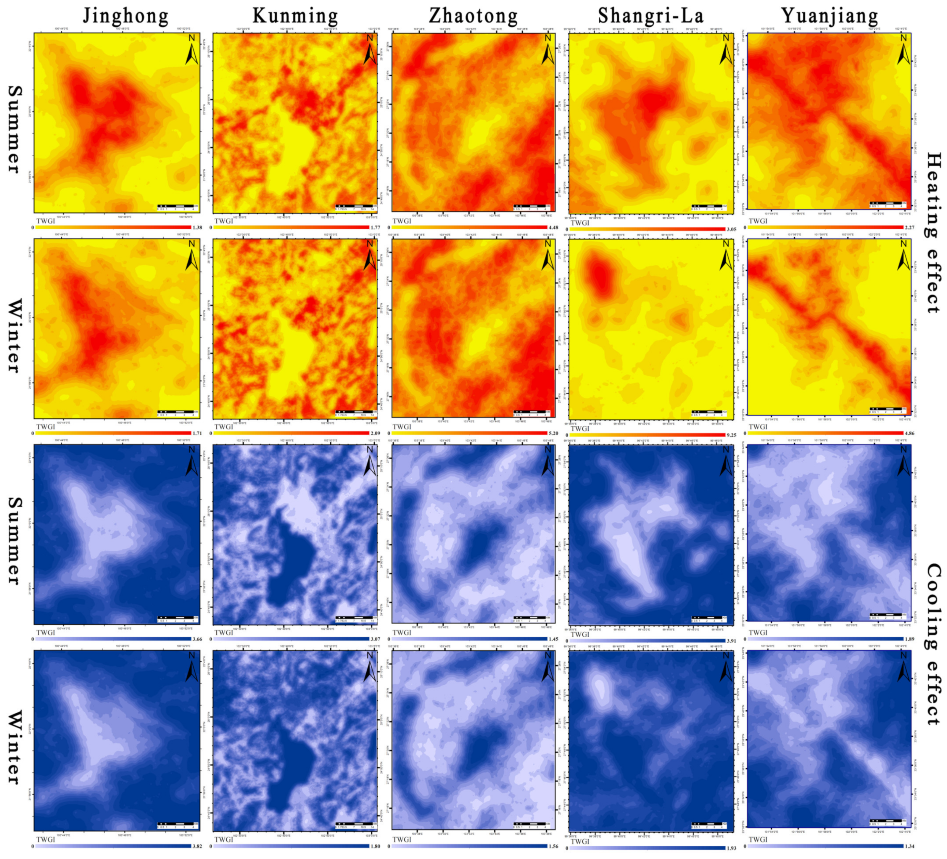
2.2.2. Distinguishing the Cooling and Heating Effects of the LCZ

TDI was adopted to compare intercity and intracity SUHI intensity values in this study [30]. The LST data were divided into four classes from low to high values with the Jenks natural break method [31], and the proportion of high-LST pixels was used to quantify the thermal contribution in Python 3.9. The TDI value of L C Z i (LCZ1–LCZH) can be estimated with Equation (5):
T D I L C Z i = A H i g h L C Z i / A L C Z i A H i g h / A
where A H i g h / A is the proportion of the area with a high LST in the entire area, and A H i g h L C Z i / A L C Z i denotes the proportion of the area with a high LST in the area of L C Z i . The contribution of L C Z i to the SUHI intensity was indicated by the T D I L C Z i value range. A value of 1 indicates a moderate contribution. If the value is higher than 1, L C Z i exhibits a heating effect. Conversely, if the value is lower than 1, L C Z i exhibits a cooling effect.

2.2.3. Quantifying the Spatial Distribution of the Heating/Cooling Effect

The gravity index (GI) referenced by Reilly’s law of retail gravitation was proposed to quantify the cooling effect of urban green spaces and waterbodies [20]. It reflects the distance and size effect of a certain land cover type on LST but ignores the influence of surface properties and surrounding environments. For example, two forest patches with the same size and distance from a specific place might have different cooling effect magnitudes due to variations in vegetation type, patch shape, tree densities, and even surrounding LCZ landscape patterns. For this reason, we used the TDI value to modify the GI. The TWGI of cell i was calculated as Equation (6) by using Python 3.9:
T W G I i = j B i A L C Z i d i j α · T D I j
where j is the surrounding cells with a buffer area of 1500 m radius, A L C Z i refers to the area of cell i with a heating/cooling effect, d i j is the distance between cell i and j, α is the adjusted distance coefficient, and T D I j is the TDI value of cell j, which is calculated in Formula (5) (Figure A2).

2.2.4. Statistical Analysis

The LST value at one specific pixel is spatially correlated with the LST values at its neighboring locations. It is necessary to verify whether the spatial regression models are more suitable than OLS linear regression models for analyzing the relationship between the TWGI and LST. Therefore, the OLS linear regression model and two types of spatial regression models, the spatial lag model (SLM) and spatial error model (SEM), were used to explain the spatial effects of heating/cooling LCZs by using GeoDa software (https://spatial.uchicago.edu/software (accessed on 22 November 2021)). The Lagrange multiple (LM) test was conducted to decide which model was appropriate [38]. Several criteria were used to choose which model is most suitable. The LM and error lag λ in Table A3 were significant, which indicated the spatial model was necessary. Moreover, the SEM’s log-likelihood was higher and the Akaike information criterion (AIC) was lower compared with the SLM (Table A4), which implied that the SEM was more suitable than other models.

3. Results

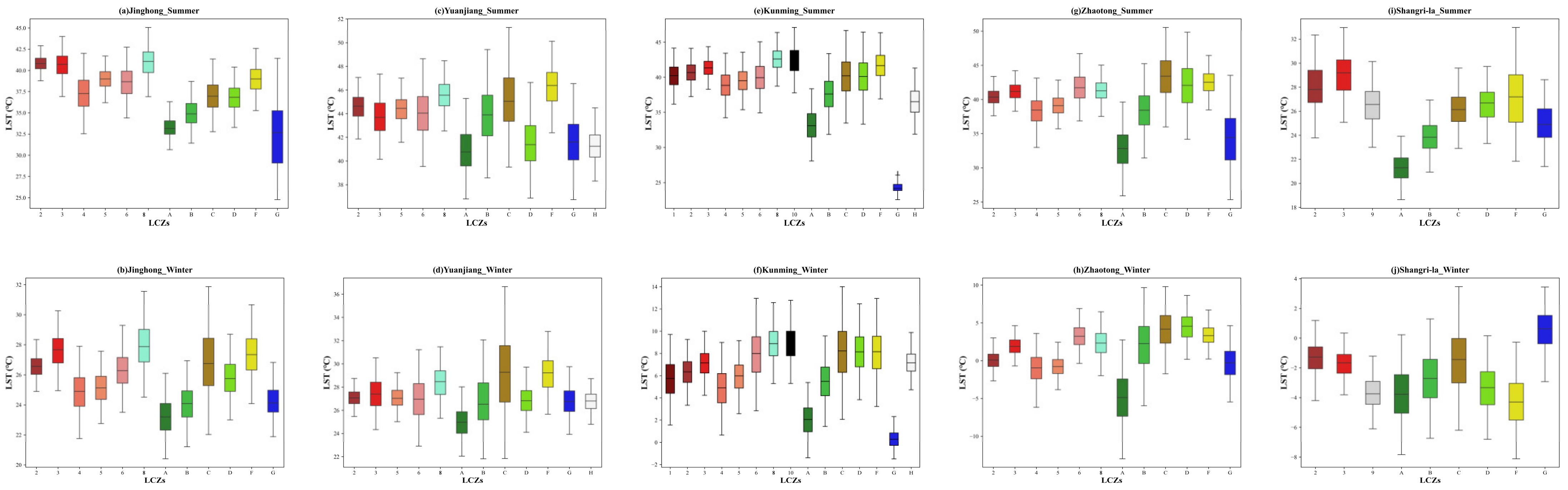
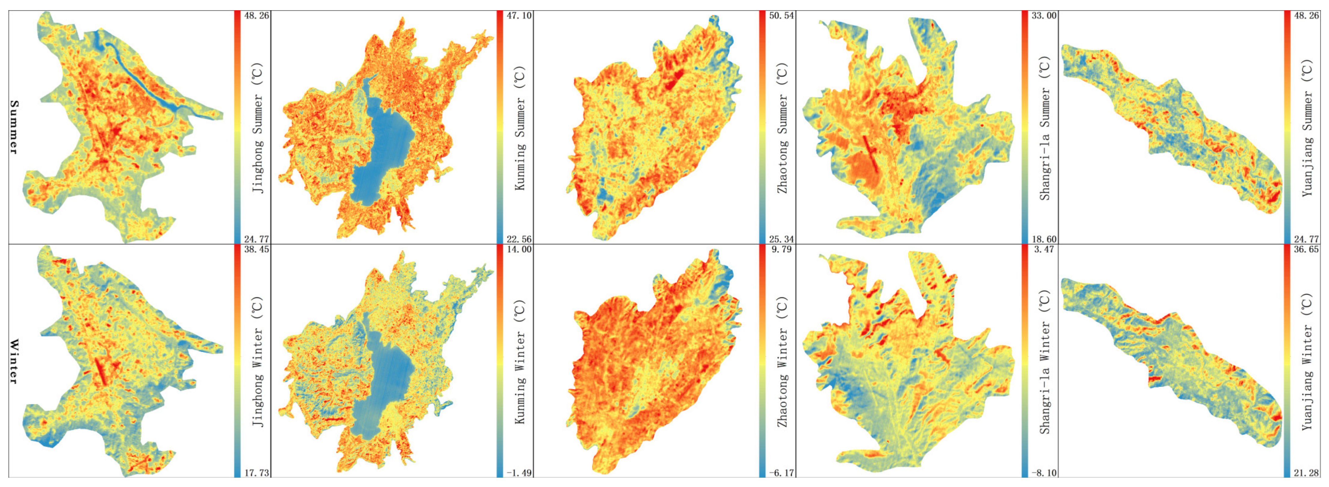
3.1. LCZ Classification and LST Investigation

LCZ maps were generated with the modified method, as shown in Figure 3. LCZ types with fewer than 10 training data items were excluded from the LCZ scheme, and a new LCZ type featuring plastic foils on farmland (LCZH) was added to the scheme due to the uncertainty in properties. The highest overall accuracies of the maps of Kunming, Shangri-La, Yuanjiang, Jinghong, and Zhaotong, with kernel sizes of 7 × 7 , 7 × 7 , 5 × 5 , 5 × 5 , and 7 × 7 , respectively, reached 92.5%, 92.5%, 89.1%, 88.2%, and 85.1%, respectively (Table A2).
The spatial patterns of the LCZs and LST values are shown in Figure 4. The analysis of variance showed that different types of LCZs exhibited distinct LST characteristics (Figure A3). The mean LST value of each LCZ was calculated for statistical analysis (Figure A1 and Table 2). The results showed that the background climate played a key role in LST variation in each LCZ. In summer, natural zones with less vegetation attained the highest LST in Yuanjiang (LCZC and LCZF) and Zhaotong (LCZC–LCZF). In the other cities, large low-rise (LCZ8) and heavy industry zones (LCZ10) obtained the highest LST, followed by compact mid-rise (LCZ2), compact low-rise (LCZ3), and bare soil (LCZF) zones. From summer to winter, built-up zones, especially open rises (LCZ4–LCZ6), tended to obtain lower LST than natural zones with less vegetation (LCZC–LCZF) in Jinghong and Kunming. However, the warmest zones were unchanged in Yuanjiang and Zhaotong. A rather interesting outcome was observed in that waterbodies (LCZG) tended to obtain the highest LST in Shangri-La in winter.

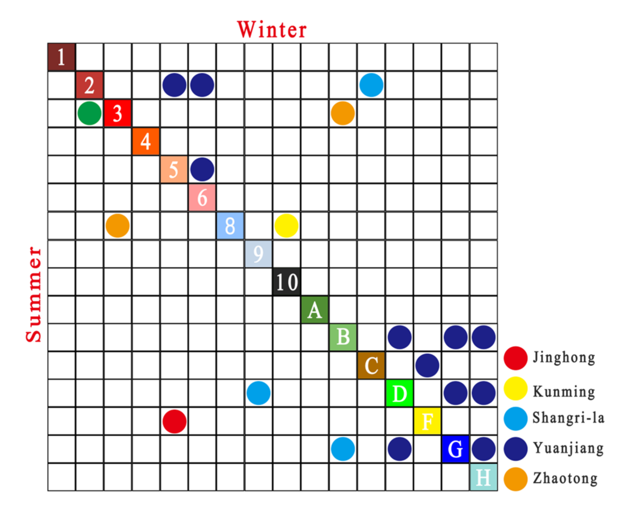
3.2. Thermal Contributions of the LCZs

The heating/cooling effect of the individual LCZs on the urban thermal environment was quantified by the TDI value (Figure 5 and Figure A2). In summer, the thermal contributions of built-up zones imposed the greatest heating effects on the SUHI phenomenon in Shangri-La and Jinghong. In contrast, most built-up zones exhibited cooling effects in Yuanjiang and Zhaotong. In Kunming, both cooling effects (LCZ4 and LCZ5) and heating effects (LCZ1–LCZ3 and LCZ6–LCZ10) were shown in built-up LCZs. For natural LCZs, waterbodies (LCZG), dense trees (LCZA), and greenhouses (LCZH) yielded cooling contributions to the SUHI phenomenon in all cities, but the opposite results occurred in LCZF. The sparse trees (LCZB) had a cooling effect in most cities except Yuanjiang. LCZC presented heating contributions in Kunming, Yuanjiang, and Zhaotong, and LCZD showed heating contributions in Kunming, Shangri-La, and Zhaotong (Figure 5a).
According to the difference in the TDI value between winter and summer (Figure 5c), the thermal contributions of built-up zones decreased from summer to winter except in large low-rise zones (LCZ8) and compact low-rise zones (LCZ3) in Jinghong and open low-rise zones (LCZ6) in Kunming. In natural zones, the thermal contributions of dense trees (LCZA) and waterbodies (LCZG) were unchanged in most cities except Shangri-La, where the DTI value of waterbodies (LCZG) increased. In contrast, the TDI values of shrubs (LCZC) increased in most cities except Zhaotong. Moreover, the thermal contributions of other natural LCZs (LCZB, LCZD, and LCZF) represented different seasonal variations among the five cities. Overall, more built-up LCZs imposed cooling effects, and the seasonal variations in the thermal contribution pattern were more striking in Jinghong, Kunming, and Shangri-La than in Zhaotong and Yuanjiang (Figure 5a,b).
In summary, built-up LCZs mainly exhibited heating effects in Jinghong and Shangri-La but cooling effects in Yuanjiang and Zhaotong in summer. Built-up LCZs imposed both heating and cooling effects in Kunming. From summer to winter, the thermal contributions of built-up LCZs tended to decrease. Therefore, most built-up LCZs imposed cooling effects in winter rather than in summer. For natural LCZs, LCZA, LCZB, and LCZG mainly yielded cooling effects regardless of season. The thermal contributions of LCZC–LCZF represented various patterns among the five cities, although they generally imposed heating effects.

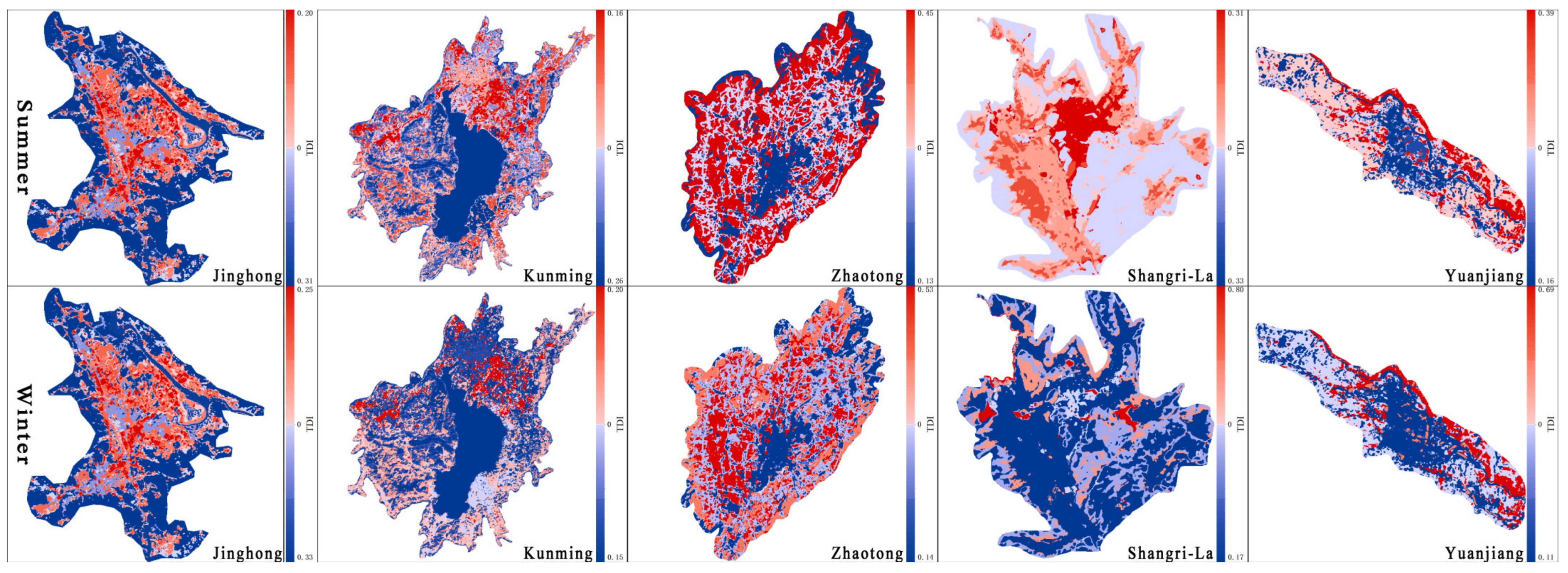
3.3. The Effect of Spatial Distribution

The spatial patterns of the TWGI values are shown in Figure 6. High TWGI values indicated that specific pixels were surrounded by clustered and large heating/cooling LCZ patches within 1500 m. The spatial patterns of the heating TWGI imposed more significant seasonal variations in Jinghong, Shangri-La, and Yuanjiang than in Kunming and Zhaotong. Moreover, the TWGI maps in blue showed that the seasonal variations in spatial patterns were more significant in Kunming and Shangri-La than in the other cities in terms of the cooling TWGI.
An appropriate regression model was used to explore the relationship between the spatial distribution of the LCZ and LST. The regression result of the SEM is shown in Table 3 and Table A4. R-square values were up to 0.99 due to the spatial autocorrelation of the error term. The TWGIs of heating/cooling LCZs had significant positive/negative impacts on the LSTs in each city (p < 0.001). The positive and negative values of the coefficient represented positive and negative correlations between the TWGI and LST. The greater the absolute values of the coefficient were, the higher the magnitude of the spatial effect (Table 3). The results of the regression analysis showed that the magnitudes of effects between heating LCZs and cooling LCZs had intercity differences and seasonal variations.
The coefficient of TWGI and its seasonal change gradient among the five cities are shown in Table 3. In summer, the spatial impacts of heating LCZs on LSTs were higher than those of cooling LCZs in Jinghong and Shangri-La, but the opposite results were observed in Yuanjiang and Kunming. In particular, the spatial effects of heating and cooling LCZs were close and low in Zhaotong but close and high in Kunming. According to the gradient of coefficient change from summer to winter, the spatial effects of heating/cooling LCZs became weaker in Yuanjiang, Kunming, and Shangri-La but stronger in Zhaotong. In Jinghong, the spatial effects of heating LCZs decreased slightly, but the opposite results were shown in cooling LCZs.

4. Discussion

4.1. Thermal Environments of the LCZs

Many studies have shown that waterbodies and green spaces play a leading role in mitigating urban heat islands by shading and evapotranspiration [8], and urban areas capture and store more heat due to the special physical properties of artificial surfaces [39,40]. However, the background climate has a large impact on the heating/cooling effects of built/nonbuilt land cover types in urban areas. For natural land cover, the background climate, such as temperature, precipitation and solar radiation, can influence photosynthesis, soil moisture and water evapotranspiration [41]. Moreover, built-up areas with different urban morphologies and surface materials have different responses to climate conditions [42]. However, it is unclear what role a certain land cover plays under different climate backgrounds, especially in urban areas with high heterogeneity. The LCZ classification scheme was used to differentiate heating/cooling effects for a certain land cover in this study. There are two reasons: (1) previous studies have shown that it is suitable for LST studies under different macroclimate regions [41], which was also improved by the ANOVA test in this study (Figure A3), and (2) it consists of various types of urban landscapes and urban forms for urban planning [21].
In summer, some studies have shown that most built-up LCZs exhibited heating effects, but natural LCZs covered with trees and waterbodies imposed cooling effects [10,11,42,43]. The same results were shown in Jinghong, Kunming, and Shangri-La. This is because built-up LCZs capture and store more solar energy, but natural LCZs increase latent heat by evapotranspiration. However, natural LCZs covered with less vegetation (LCZC–LCZF) mainly presented heating effects, and built-up LCZs imposed cooling effects in Yuanjiang and Zhaotong. This is because dry soil has a low heat capacity and low vegetation activity in arid cities [41]. Moreover, a previous study suggested that a rough built-up area could enhance the convection efficiency and lower the aerodynamic resistance in dry climate zones, resulting in a cooling effect on impervious surfaces [17]. In addition, urban green space management could lead to higher evapotranspiration compared with natural LCZs in Yuanjiang and Zhaotong. Furthermore, the heating effects of LCZC and LCZF were higher in Yuanjiang than in Zhaotong because the higher temperature in Yuanjiang could enhance the degree of dryness and lead to lower vegetation activity compared with Zhaotong. For this reason, even the scattered trees (LCZB) imposed heat effects regardless of season in Yuanjiang.
From summer to winter, there was a trend of decreasing heating effects of built-up LCZs in Jinghong, Kunming, and Shangri-La. This result was also suggested by a study conducted in Nanjing [43]. One possible reason is that built-up LCZs capture and store less solar radiation in winter than in summer. The thermal contributions of low plants (LCZD) and bare soil (LCZF) decreased in Shangri-La, possibly due to snow. The surface albedo of areas covered with snow was high. Moreover, waterbodies (LCZG) obtained the highest LST in Shangri-La in winter. This is because vertical convection and mixing of the lake water occur during the overturning period to ensure that the surface temperature of the lake is not too low [44]. However, other LCZs covered with snow corresponded to lower LSTs due to their high albedo.
Spatial distribution, background climate and human activities jointly impacted LST variations. For example, low plants (LCZD) without interference showed a heating effect in Yuanjiang, but LCZD with good irrigation (farmland) belonged to cooling LCZ. Notably, there was a large area of farmland with less irrigation in Zhaotong, which caused higher LSTs in the suburbs than in urban areas. Moreover, previous studies have demonstrated that the mean LST decreases with increasing openness and height of built-up zones [42,43]. However, open low-rise zones (LCZ6) surrounded by low plants (LCZD) constituted the warmest zone in Zhaotong. The climatic background resulted in a significant heating effect of low plants (LCZD), and the landscape distribution increased the LST of open low-rise plants (LCZ6). Moreover, compact low-rise zones (LCZ3) surrounded by low plants (LCZD) with good irrigation obtained the lowest mean LST in Yuanjiang. Low plants (LCZD) yielded a cooling effect due to agricultural activities, and the LST in compact low-rise zones (LCZ3) decreased due to the spatial effects of LCZD. For this reason, it is important to quantify the relationship between the spatial distribution of heating/cooling LCZs and LSTs.

4.2. Spatial Effects of Heating/Cooling LCZs on LSTs

The spatial distribution of heating/cooling LCZs can change the aerodynamics in urban areas, which further impacts LSTs [45]. However, their spatial effect is seldom studied. Should urban planners pay more attention to the urban land arrangement and should heating land or cooling land be focused under different background climates? To answer this question, a more reliable index (TWGI) was proposed, and SEM was used to analyze the relationship between TWGI and LST in this study.
The high TWGI value indicated that the specific pixel was surrounded by clustered and large heating/cooling LCZ patches within 1500 m. Some studies have indicated that clustered vegetation decreases the overall evapotranspiration rate and weakens the cooling benefits from vegetation, but clustered built-up areas elevate LST in humid and hot cities [46,47]. Therefore, the spatial heating effects of the built-up LCZs were higher than the spatial cooling effects of the natural LCZs in Jinghong. Similar results were also shown in Shangri-La, but these results could have been caused by the low vegetation activities in alpine regions. Clustered impervious areas, vegetation and waterbodies cannot effectively lower LST in arid cities of the USA [46]. For this reason, the spatial effects of heating/cooling LCZs were low in Zhaotong. However, the spatial effects of cooling LCZs were high in Yuanjiang. One possible reason is that a large area of farmland with good irrigation may enhance evapotranspiration in Yuanjiang.

4.3. Contributions and Limitations

A standard framework for distinguishing between the cooling effect and heating effect and spatial effect analysis based on the LCZ scheme was conducted in this study. The results of the spatial effect and thermal contributions can better help make target mitigation strategies for distinct macroclimate cities. In particular, an index (TWGI) was proposed to quantify the spatial effects of heating/cooling LCZs. The higher value of log-likelihood and lower value of the Akaike information criterion indicated that TWGI could better explain the spatial effect of heating/cooling LCZs than traditional GI (Table A4) [20,38]. The results based on the GI value cannot reflect the exact heating/cooling effect owing to ignoring the magnitude of thermal contributions.
Long time series of LST data are recommended for LCZ surface temperature studies to reduce uncertainty [25]. In this study, multiyear Landsat8 images were searched for LST retrievals from 2018 to 2020. Fewer images were available due to cloud cover, especially in summer. For this reason, the LSTs were retrieved using single-time images, which might cause uncertainties [41]. However, the uncertainty caused by Landsat 8 images with a restricted temporal scale can be considered negligible in this study due to the following reasons: (1) The results of the ANOVA test showed a typical LST regime for each LCZ in all cities, which implied that the results of mean LST per LCZ were acceptable; and (2) the dramatic land cover and land use changes might increase uncertainty over the results of LCZ LSTs in developing cities [5]. Furthermore, climatic conditions are a dominant factor causing different thermal contributions of the LCZs and spatial effects among the five cities, but other factors, such as geographical locations and human activities, can also influence the thermal environments of specific LCZs. However, the actual causes need to be investigated.

5. Conclusions

First, the heating/cooling contributions of typical LCZs in five Chinese cities were distinguished. Second, a TWGI was proposed to quantify the spatial effects of heating/cooling LCZs on LSTs. In summary, both the thermal contributions of LCZs and their spatial heating/cooling effects were different in the five cities. The conclusions are as follows:
(1) In summer, built-up zones are characterized as heating LCZs in Jinghong and Shangri-La, but opposite results were shown in Zhaotong and Yuanjiang. Moreover, most of the built-up LCZs experienced heating effects in Kunming, except for open mid-rise (LCZ4) and low-rise (LCZ5). For natural LCZs, areas covered with dense trees (LCZA), scattered trees (LCZB), and waterbodies (LCZG) presented cooling effects. However, the thermal contributions of shrubs (LCZC), low plants (LCZD), and bare soil (LCZF) varied among the five cities because they are sensitive to background climate change and human activities.
(2) The results of the SEMs showed that urban planners should pay more attention to the spatial distribution of heating LCZs in Jinghong and Shangri-La, but the spatial distribution of cooling LCZs was more important in Yuanjiang and Kunming. Moreover, both cooling LCZs and heating LCZs had slight spatial impacts on LSTs in Zhaotong, which implies that enhancing the evaporation capability could be a more efficient way to mitigate SUHIs in Zhaotong.
(3) From summer to winter, built-up zones tended to have lower thermal contributions. However, the cooling effects of trees (LCZA, LCZB) and waterbodies (LCZG) were almost unchanged. The LST differences between natural LCZs and built-up LCZs decreased to induce low aerodynamics. For this reason, the spatial effects of heating/cooling LCZs weakened.

Author Contributions

Conceptualization, N.L. and B.W.; methodology, N.L.; software, N.L. and Y.Y.; validation, N.L., Y.Y. and B.W.; investigation, N.L.; writing—original draft preparation, N.L. and B.W.; writing—review and editing, L.C., Y.Y. and Z.Z.; visualization, N.L.; supervision, Z.Z. and L.C. All authors have read and agreed to the published version of the manuscript.

Funding

This work was supported by the Second Tibetan Plateau Scientific Expedition and Research program (No. 2019QZKK0308).

Data Availability Statement

The Landsat 8 data presented in this study are available through USGS, https://earthexplorer.usgs.gov/ (accessed on 12 October 2021).

Acknowledgments

We appreciate the critical and constructive comments and suggestions from the reviewers that helped improve the quality of this manuscript.

Conflicts of Interest

The authors declare no conflict of interest.

Appendix A. LCZ and LST Mapping

Table A1. Information on Landsat images for LCZ mapping and LST retrieval.
CityScene IDAcquisition DataScene Time (UTC)Images for LST Retrieval
JinghongLC81300452019358LGN002019-12-2403:42Winter
LC81300452020137LGN002020-05-1603:41Summer
LC81300452019038LGN002019-02-0703:41
KunmingLC81290432019351LGN002019-12-1703:35Winter
LC81290432019127LGN002019-05-0703:34Summer
LC81290432019047LGN002019-02-1603:34
ZhaotongLC81290412019079LGN002019-03-2003:33
LC81290412020130LGN002020-05-0903:33Summer
LC81290412019223LGN002019-08-1103:34
LC81290412019351LGN002019-12-1703:34Winter
Shangri-LaLC81320412019228LGN002019-08-1603:52Summer
LC81320412020087LGN002020-03-2703:52
LC81320412020007LGN002020-01-0703:52Winter
YuanjiangLC81300442019358LGN002019-12-2403:41Winter
LC81300442020073LGN002020-03-1303:41
LC81300442020137LGN002020-05-1604:40Summer
Table A2. The accuracy of LCZ classifications (NA represents no-data value).
LCZsWUDAPTModified Method
JinghongYuanjiangKunmingZhaotongShangri-LaJinghongYuanjiangKunmingZhaotongShangri-La
LCZ1NANA40.48NANANANA57.96NANA
LCZ273.9662.6957.2860.9875.5482.9891.0761.0274.6390.00
LCZ373.5369.8464.6064.0073.0279.0773.2174.0483.0474.59
LCZ473.75NA49.7980.87NA78.67NA64.4290.33NA
LCZ571.3482.8945.1389.34NA78.9297.6256.5699.17NA
LCZ671.4866.9065.1564.89NA78.4977.9358.6664.21NA
LCZ889.0059.6879.0792.04NA95.4361.7678.7195.35NA
LCZ9NANANANA89.67NANANANA98.71
LCZ10NANA85.66NANANANA89.1NANA
LCZA97.6192.4698.6898.4299.4295.8693.3398.3899.08100.00
LCZB93.1850.9637.4876.9265.9385.7176.5852.3678.9580.49
LCZC72.7398.6073.0158.9391.4591.3096.3270.8153.4794.62
LCZD45.9577.6577.8396.1010048.9480.6874.8394.66100.00
LCZF97.2790.0059.0164.3889.1398.2889.5862.4573.6197.56
LCZG99.1391.1399.9495.8398.6498.55100.0099.99100.0098.65
LCZHNA78.1398.49NANANA92.0099.51NANA
Overall accuracy (%)85.0081.3290.981.0486.50.8889.1492.585.1891.75
Kappa Coefficient0.830.790.800.790.840.870.880.840.830.90

Appendix B. Land Surface Temperature and Local Climate Zones

To study the thermal characteristics of all LCZs, the mean values of the LST for each LCZ were calculated (Table 2), and the statistical significance of differences among them was determined by an ANOVA test [43]. The Kolmogorov–Smirnov test was used as a normality test, and Levene’s test was used to assess the homogeneity of the variance. The Kolmogorov–Smirnow test was rejected in this study, but the data were considered to approximately obey a normal distribution because the absolute values of skewness and kurtosis were less than one. Welch ANOVA was then applied to determine whether there was a significant difference among the mean LSTs, and Tamhane’s T2 test was used for pairwise comparisons of mean LSTs due to the rejection of Levene’s test (Figure A3). The results of the Welch ANOVA test showed a typical LST regime for each LCZ in all the cities. The results of Tamhane’s T2 test showed that most LCZs were better distinguished in Pu’er regardless of season, followed by Jinghong, Kunming, and Shangri-La. However, some LCZs were not indistinguishable in Yuanjiang.
Figure A1. Boxplots of the LST values of the typical LCZs in the different seasons.
Remotesensing 14 04029 g0a1
Figure A2. The TDI distributions in five cities (the red color represents LCZs with heating effects, and the blue color represents LCZs with cooling effects).
Remotesensing 14 04029 g0a2
Figure A3. Multiple-comparison results of the differences in the mean LST among the various LCZ types (white numbers and letters). The solid-colored circles represent no significant difference in mean LST, and the hollow cells show that the mean LSTs of the given LCZ pairs were significantly different.
Remotesensing 14 04029 g0a3

Appendix C. Spatial Regression Validation

Table A3. The results of SEM (*** p < 0.001, ** p < 0.01, R-squared values of OLS are presented in parentheses).
SeasonCityThermal ContributionCoefficientConstantλLMR-SquaredLog-LikelihoodAIC
SummerJHHeating LCZs13.2733.16 ***1.00 ***375.64 ***0.99
(0.50)
59,092.98−118,178.00
Cooling LCZs−1.81
YJHeating LCZs1.5149.27 ***1.00 ***56.75 ***0.99
(0.12)
7909.14−15,812.30
Cooling LCZs−12.73
KMHeating LCZs7.8948.34 ***1.00 ***39,717.31 ***0.99
(0.38)
−159,410.66318,827.00
Cooling LCZs−12.73
ZTHeating LCZs0.2840.63 ***1.00 ***6.31 **0.99
(0.20)
5380.81−10,755.60
Cooling LCZs−0.19
SGHeating LCZs8.5819.93 ***1.00 ***1240.17 ***0.99
(0.58)
126,248.96−252,492.00
Cooling LCZs−0.92
WinterJHHeating LCZs9.1233.16 ***1.00 ***482.91 ***0.99
(0.42)
59,092.98−118,178.00
Cooling LCZs−1.99
YJHeating LCZs0.5249.27 ***1.00 ***13.43 ***0.99
(0.16)
7909.14−15,812.30
Cooling LCZs−4.30
KMHeating LCZs5.4648.34 ***1.00 ***30,623.04 ***0.99
(0.25)
−159,410.66318,827.00
Cooling LCZs−4.72
ZTHeating LCZs0.3840.63 ***1.00 ***6.31 **0.99
(0.37)
5380.81−10,755.60
Cooling LCZs−0.42
SGHeating LCZs2.3919.93 ***1.00 ***1240.17 ***0.99
(0.33)
126,248.96−252,492.00
Cooling LCZs−0.57
Table A4. Comparison of the results of SEMs based on GI and TWGI in Jinghong (*** p < 0.001, R-squared values of OLS are presented in parentheses).
Index Thermal ContributionCoefficientConstantλR-SquaredLog-LikelihoodAIC
TWGISummerHeating LCZs13.27 ***33.16 ***1.00 ***0.99
(0.50)
59,092.98−118,178.00
Cooling LCZs−1.81 ***
WinterHeating LCZs9.12 ***24.51 ***1.00 ***0.99
(0.42)
63,098.09−126,188.00
Cooling LCZs−1.99 ***
GISummerHeating LCZs1.36 ***33.87 ***1.00 ***0.99
(0.45)
58,009.12−116,010.00
Cooling LCZs−0.41 ***
WinterHeating LCZs0.89 ***25.70 ***1.00 ***0.99
(0.41)
60,165.67−120,325.00
Cooling LCZs−0.48 ***

References

  1. United Nations Department of Economic and Social Affairs. World Urbanization Prospects 2018: Highlights; United Nations: New York, NY, USA, 2019. [Google Scholar] [CrossRef]
  2. Oke, T.R. The energetic basis of the urban heat island. Q. J. Meteorol. Soc. 1982, 108, 1–24. [Google Scholar] [CrossRef]
  3. Basara, J.B.; Basara, H.G.; Illston, B.G.; Crawford, K.C. The Impact of the Urban Heat Island during an Intense Heat Wave in Oklahoma City. Adv. Meteorol. 2010, 2010, 230365. [Google Scholar] [CrossRef]
  4. Roxon, J.; Ulm, F.J.; Pellenq, R.J.M. Urban heat island impact on state residential energy cost and CO2 emissions in the United States. Urban Clim. 2020, 31, 100546. [Google Scholar] [CrossRef]
  5. Zhou, D.; Xiao, J.; Bonafoni, S.; Berger, C.; Deilami, K.; Zhou, Y.; Frolking, S.; Yao, R.; Qiao, Z.; Sobrino, J. Satellite Remote Sensing of Surface Urban Heat Islands: Progress, Challenges, and Perspectives. Remote. Sens. 2018, 11, 48. [Google Scholar] [CrossRef]
  6. Marshall, B.; Ezekiel, C.; Gichuki, J.; Mkumbo, O.; Sitoki, L.; Wanda, F. Global warming is reducing thermal stability and mitigating the effects of eutrophication in Lake Victoria (East Africa). Nat. Preced. 2009. [Google Scholar] [CrossRef]
  7. Deilami, K.; Kamruzzaman, M.; Liu, Y. Urban heat island effect: A systematic review of spatio-temporal factors, data, methods, and mitigation measures. Int. J. Appl. Earth Obs. Geoinf. 2018, 67, 30–42. [Google Scholar] [CrossRef]
  8. Su, Y.; Wu, J.; Zhang, C.; Wu, X.; Li, Q.; Liu, L.; Bi, C.; Zhang, H.; Lafortezza, R.; Chen, X. Estimating the cooling effect magnitude of urban vegetation in different climate zones using multi-source remote sensing. Urban Clim. 2022, 43, 101155. [Google Scholar] [CrossRef]
  9. Wang, C.; Wang, Z.-H.; Yang, J. Cooling Effect of Urban Trees on the Built Environment of Contiguous United States. Earth’s Future 2018, 6, 1066–1081. [Google Scholar] [CrossRef]
  10. Cai, M.; Ren, C.; Xu, Y.; Lau, K.K.-L.; Wang, R. Investigating the relationship between local climate zone and land surface temperature using an improved WUDAPT methodology—A case study of Yangtze River Delta, China. Urban Clim. 2018, 24, 485–502. [Google Scholar] [CrossRef]
  11. Chen, X.; Xu, Y.; Yang, J.; Wu, Z.; Zhu, H. Remote sensing of urban thermal environments within local climate zones: A case study of two high-density subtropical Chinese cities. Urban Clim. 2020, 31, 100568. [Google Scholar] [CrossRef]
  12. Nassar, A.K.; Blackburn, G.A.; Whyatt, J.D. Dynamics and controls of urban heat sink and island phenomena in a desert city: Development of a local climate zone scheme using remotely-sensed inputs. Int. J. Appl. Earth Obs. Geoinf. 2016, 51, 76–90. [Google Scholar] [CrossRef]
  13. Yang, Q.; Huang, X.; Li, J. Assessing the relationship between surface urban heat islands and landscape patterns across climatic zones in China. Sci. Rep. 2017, 7, 9337. [Google Scholar] [CrossRef] [PubMed]
  14. O′Neill, R.V.; Krummel, J.R.; Gardner, R.H.; Sugihara, G.; Jackson, B.; DeAngelis, D.L.; Milne, B.T.; Turner, M.G.; Zygmunt, B.; Christensen, S.W.; et al. Indices of landscape pattern. Landsc. Ecol. 1988, 1, 153–162. [Google Scholar] [CrossRef]
  15. Du, H.; Wang, D.; Wang, Y.; Zhao, X.; Qin, F.; Jiang, H.; Cai, Y. Influences of land cover types, meteorological conditions, anthropogenic heat and urban area on surface urban heat island in the Yangtze River Delta Urban Agglomeration. Sci. Total Environ. 2016, 571, 461–470. [Google Scholar] [CrossRef] [PubMed]
  16. Li, J.; Song, C.; Cao, L.; Zhu, F.; Meng, X.; Wu, J. Impacts of landscape structure on surface urban heat islands: A case study of Shanghai, China. Remote. Sens. Environ. 2011, 115, 3249–3263. [Google Scholar] [CrossRef]
  17. Zhao, L.; Lee, X.; Smith, R.B.; Oleson, K. Strong contributions of local background climate to urban heat islands. Nature 2014, 511, 216–219. [Google Scholar] [CrossRef] [PubMed]
  18. Peng, S.-S.; Piao, S.; Zeng, Z.; Ciais, P.; Zhou, L.; Li Laurent, Z.X.; Myneni Ranga, B.; Yin, Y.; Zeng, H. Afforestation in China cools local land surface temperature. Proc. Nat. Acad. Sci. USA 2014, 111, 2915–2919. [Google Scholar] [CrossRef]
  19. Gunawardena, K.R.; Wells, M.J.; Kershaw, T. Utilising green and bluespace to mitigate urban heat island intensity. Sci. Total Environ. 2017, 584, 1040–1055. [Google Scholar] [CrossRef]
  20. Wang, Y.; Zhan, Q.; Ouyang, W. How to Quantify the relationship between spatial distribution of urban waterbodies and land surface temperature? Sci. Total Environ. 2019, 671, 1–9. [Google Scholar] [CrossRef]
  21. Aslam, A.; Rana, I.A. The use of local climate zones in the urban environment: A systematic review of data sources, methods, and themes. Urban Clim. 2022, 42, 101120. [Google Scholar] [CrossRef]
  22. Oke, T.R.; Mills, G.; Christen, A.; Voogt, J.A. Urban Climates; Cambridge University Press: Cambridge, UK, 2017. [Google Scholar]
  23. Stewart, I.D.; Oke, T.R.; Krayenhoff, E.S. Evaluation of the ‘local climate zone’ scheme using temperature observations and model simulations. Int. J. Climatol. 2014, 34, 1062–1080. [Google Scholar] [CrossRef]
  24. Bechtel, B.; Alexander, P.J.; Beck, C.; Böhner, J.; Brousse, O.; Ching, J.; Demuzere, M.; Fonte, C.; Gál, T.; Hidalgo, J.; et al. Generating WUDAPT level 0 data—Current status of production and evaluation. Urban Clim. 2019, 27, 24–45. [Google Scholar] [CrossRef]
  25. Bechtel, B.; Demuzere, M.; Mills, G.; Zhan, W.; Sismanidis, P.; Small, C.; Voogt, J. SUHI analysis using Local Climate Zones—A comparison of 50 cities. Urban Clim. 2019, 28, 100451. [Google Scholar] [CrossRef]
  26. Lin, Z.; Xu, H. A Study of urban heat island intensity based on “local climate zones”: A case study in Fuzhou, China. In Proceedings of the 4th International Workshop on Earth Observation and Remote Sensing Applications (EORSA), Guangzhou, China, 4–6 July 2016; pp. 250–254. [Google Scholar] [CrossRef]
  27. Ochola, E.M.; Fakharizadehshirazi, E.; Adimo, A.O.; Mukundi, J.B.; Wesonga, J.M.; Sodoudi, S. Inter-Local climate zone differentiation of land surface temperatures for management of Urban Heat in Nairobi City, Kenya. Urban Clim. 2020, 31, 100540. [Google Scholar] [CrossRef]
  28. Shih, W. The impact of urban development patterns on thermal distribution in Taipei. In Proceedings of the 2017 Joint Urban Remote Sensing Event (JURSE), Dubai, United Arab Emirates, 6–8 March 2017; pp. 1–5. [Google Scholar] [CrossRef]
  29. Wang, C.; Middel, A.; Myint, S.W.; Kaplan, S.; Brazel, A.J.; Lukasczyk, J. Assessing local climate zones in arid cities: The case of Phoenix, Arizona and Las Vegas, Nevada. ISPRS J. Photogr. Remote Sens. 2018, 141, 59–71. [Google Scholar] [CrossRef]
  30. Zhao, C. Linking the Local Climate Zones and Land Surface Temperature to Investigate the Surface Urban Heat Island, a Case Study of San Antonio, Texas, U.S. ISPRS Ann. Photogr. Remote Sens. Spat. Inf. Sci. 2018, 3, 277–283. [Google Scholar] [CrossRef]
  31. Zhao, C.; Jensen, J.L.R.; Weng, Q.; Currit, N.; Weaver, R. Use of Local Climate Zones to investigate surface urban heat islands in Texas. GIScience Remote Sens. 2020, 57, 1083–1101. [Google Scholar] [CrossRef]
  32. Zomer, R.J.; Xu, J.; Wang, M.; Trabucco, A.; Li, Z. Projected impact of climate change on the effectiveness of the existing protected area network for biodiversity conservation within Yunnan province, China. Biol. Conserv. 2015, 184, 335–345. [Google Scholar] [CrossRef]
  33. Xu, D.; Yun, T.; Chang-chun, D. A fine mesh climate division and the selection of representative climate stations in Yunnan Province. Trans. Atmos. Sci. 2011, 34, 336–342. [Google Scholar]
  34. Verdonck, M.-L.; Okujeni, A.; Van der Linden, S.; Demuzere, M.; De Wulf, R.; van Coillie, F. Influence of neighbourhood information on ‘Local Climate Zone’ mapping in heterogeneous cities. Int. J. Appl. Earth Obs. Geoinf. 2017, 62, 102–113. [Google Scholar] [CrossRef]
  35. Stewart, I.D.; Oke, T.R. Local Climate Zones for Urban Temperature Studies. Bull. Am. Meteorol. Soc. 2012, 93, 1879–1900. [Google Scholar] [CrossRef]
  36. Du, C.; Ren, H.; Qin, Q.; Meng, J.; Zhao, S. A Practical Split-Window Algorithm for Estimating Land Surface Temperature from Landsat 8 Data. Remote Sens. 2015, 7, 647–665. [Google Scholar] [CrossRef]
  37. Ren, H.; Du, C.; Liu, R.; Qin, Q.; Yan, G.; Li, Z.-L.; Meng, J. Atmospheric water vapor retrieval from Landsat 8 thermal infrared images. J. Geophys. Res. Atmos. 2015, 120, 1723–1738. [Google Scholar] [CrossRef]
  38. Dai, Z.; Guldmann, J.-M.; Hu, Y. Spatial regression models of park and land-use impacts on the urban heat island in central Beijing. Sci. Total Environ. 2018, 626, 1136–1147. [Google Scholar] [CrossRef]
  39. Yang, J.; Ren, J.; Sun, D.; Xiao, X.; Xia, J.; Jin, C.; Li, X. Understanding land surface temperature impact factors based on local climate zones. Sustain. Cities Soc. 2021, 69, 102818. [Google Scholar] [CrossRef]
  40. Yang, J.; Wang, Y.; Xiao, X.; Jin, C.; Xia, J.; Li, X. Spatial differentiation of urban wind and thermal environment in different grid sizes. Urban Clim. 2019, 28, 100458. [Google Scholar] [CrossRef]
  41. Eldesoky, A.H.M.; Gil, J.; Pont, M.B. The suitability of the urban local climate zone classification scheme for surface temperature studies in distinct macroclimate regions. Urban Clim. 2021, 37, 100823. [Google Scholar] [CrossRef]
  42. Khoshnoodmotlagh, S.; Daneshi, A.; Gharari, S.; Verrelst, J.; Mirzaei, M.; Omrani, H. Urban morphology detection and it′s linking with land surface temperature: A case study for Tehran Metropolis, Iran. Sustain. Cities Soc. 2021, 74, 103228. [Google Scholar] [CrossRef]
  43. Du, P.; Chen, J.; Bai, X.; Han, W. Understanding the seasonal variations of land surface temperature in Nanjing urban area based on local climate zone. Urban Clim. 2020, 33, 100657. [Google Scholar] [CrossRef]
  44. Wetzel, R.G. 6—Fate of Heat. In Limnology, 3rd ed.; Wetzel, R.G., Ed.; Academic Press: San Diego, CA, USA, 2001; pp. 71–92. [Google Scholar]
  45. Li, D.; Liao, W.; Rigden, A.J.; Liu, X.; Wang, D.; Malyshev, S.; Shevliakova, E. Urban heat island: Aerodynamics or imperviousness? Sci. Adv. 2019, 5, eaau4299. [Google Scholar] [CrossRef]
  46. Wang, C.; Li, Y.; Myint, S.W.; Zhao, Q.; Wentz, E.A. Impacts of spatial clustering of urban land cover on land surface temperature across Köppen climate zones in the contiguous United States. Landsc. Urban Plan. 2019, 192, 103668. [Google Scholar] [CrossRef]
  47. Hwang, Y.H.; Lum, Q.J.G.; Chan, Y.K.D. Micro-scale thermal performance of tropical urban parks in Singapore. Build. Environ. 2015, 94, 467–476. [Google Scholar] [CrossRef]
Figure 1. Geographic distribution of the cities considered in this study along with their background climate (SRL: Shangri-La; ZT: Zhaotong; KM: Kunming; YJ: Yuanjiang; JH: Jinghong; MATP: Mean annual precipitation; Data source: http://www.resdc.cn/ (accessed on 12 October 2021), DOI: 10.12078/2017121301).
Remotesensing 14 04029 g001
Figure 2. (a) LCZ scheme adapted with permission from Ref. [35]. 2022, Stewart; (b) Workflow of the moving window method based on the WUDAPT adapted with permission from Ref. [34]. 2022, Verdonck.
Remotesensing 14 04029 g002
Figure 3. LCZ classification of the five cities in Yunnan Province (a) Jinghong, (b) Kunming, (c) Zhaotong, (d) Shangri-La, (e) Yuanjiang).
Remotesensing 14 04029 g003
Figure 4. LST values in summer and winter in the cities with different background climates (units: °C).
Remotesensing 14 04029 g004
Figure 5. TDI values of each LCZ in summer (a) and winter (b) in the five cities with different background climates (black indicates no-data value, red indicates heating contribution, blue indicates cooling contribution, TDI values are shown in each box); (c) difference in the value of the thermal distribution index (TDI) between winter and summer (black indicates no-data value, red and blue indicate the increase and decrease of TDI values from summer to winter).
Remotesensing 14 04029 g005
Figure 6. The TWGI distributions in five cities (the red color represents the heating effect, and the blue color represents the cooling effect).
Remotesensing 14 04029 g006
Table 1. Information on the selected cities.
CityDays of ATC10 °C ATC10 °C (°C)Altitude (m)MATP 1 (mm)Climate Zone
Yuanjiang>2188844.2<500864.4Tropic (Arid)
Jinghong>2188373.6500–30001198.0Tropic
Kunming>2185558.6500–30001002.2Mid-subtropic
Zhaotong>2183914.8≥3000742.8Temperate zone
Shangri-La>1401916.0≥3000617.0Alpine zone
1 MATP: Mean annual precipitation.
Table 2. Mean LST per LCZ in winter and summer (NA represents no-data value, unit: °C).
LCZJinghongKunmingZhaotongShangri-LaYuanjiang
SummerWinterSummerWinterSummerWinterSummerWinterSummerWinter
LCZ1 (compact high-rise)NANA40.25.7NANANANANANA
LCZ2 (compact mid-rise)40.8 126.640.76.340.40.0127.9 1−1.4 144.527.1
LCZ3 (compact low-rise)40.6 127.6 141.37.141.21.929.0 1−1.843.727.4
LCZ4 (open high-rise)37.324.938.94.938.2−1.1 2NANANANA
LCZ5 (open mid-rise)39.025.139.55.939.1−0.7NANA44.327.1
LCZ6 (open low-rise)38.626.340.07.941.83.3NANA44.127.0
LCZ8 (large low-rise)41.0 128.0 142.6 18.9 141.32.3NANA45.6 128.4 1
LCZ9 (sparsely built)NANANANANANA26.5−3.7NANA
LCZ10 (heavy industry)NANA42.4 18.9 1NANANANANANA
LCZA (dense trees)33.3 223.2 233.2 22.0 232.8 2−5.0 221.2 2−3.8 240.9 225.0 2
LCZB (scattered trees)35.024.1 237.65.538.41.923.8 2−2.643.926.8
LCZC (bush, scrub)37.026.940.18.1 143.3 14.1 126.2−1.4 145.2 129.2 1
LCZD (low plants)36.825.840.08.1 142.0 14.2 126.5−3.341.626.8 2
LCZF (Bare soil or sand)39.027.4 141.7 18.1 142.5 13.4 127.0 1−4.3 246.3 129.1 1
LCZG (water)32.3 224.324.4 20.3 234.3 2−0.323.8 21.8 141.626.8 2
LCZH (greenhouse)NANA36.57.2NANANANA41.4 226.8 2
1 The warmest LCZs ranked as the top three. 2 The coldest LCZs ranked as the top two.
Table 3. The results of the SEM in five cities.
CityThermal ContributionCoefficient (Summer)Coefficient (Winter)Seasonal Change Gradient
JinghongHeating13.279.12−0.31
Cooling−1.81−1.990.10
YuanjiangHeating1.510.52−0.66
Cooling−12.73−4.30−0.66
KunmingHeating7.895.46−0.31
Cooling−12.73−4.72−0.63
ZhaotongHeating0.280.380.36
Cooling−0.19−0.421.21
Shangri-LaHeating8.582.39−0.72
Cooling−0.92−0.57−0.38
Publisher’s Note: MDPI stays neutral with regard to jurisdictional claims in published maps and institutional affiliations.

