Abstract
Space-time adaptive processing (STAP) algorithms based on sparse recovery (SR) have been researched because of their low requirement of training snapshots. However, once some portion of clutter is not located on the grids, i.e., off-grid problems, the performances of most SR-STAP algorithms degrade significantly. Reducing the grid interval can mitigate off-grid effects, but brings strong column coherence of the dictionary, heavy computational load, and heavy storage load. A sparse Bayesian learning approach is proposed to mitigate the off-grid effects in the paper. The algorithm employs an efficient sequential addition and deletion of dictionary atoms to estimate the clutter subspace, which means that strong column coherence has no effect on the performance of the proposed algorithm. Besides, the proposed algorithm does not require much computational load and storage load. Off-grid effects can be mitigated with the proposed algorithm when the grid-interval is sufficiently small. The excellent performance of the novel algorithm is demonstrated on the simulated data.
1. Introduction
Space-time adaptive processing (STAP) exhibits great potential in suppressing clutter and detecting slow-moving targets []. The Reed–Mallet–Brennan (RMB) rule [] states that signal-to-clutter-plus-noise ratio (SCNR) loss can be within 3 dB only if the number of independent and identically distributed (i.i.d) training snapshots is at least twice the system degrees of freedom (DOFs). Unfortunately, due to array configurations and the complex clutter environment, sufficient training snapshots cannot be guaranteed, and therefore the performance of STAP degrades significantly.
Motivated by compressed sensing (CS) theory, STAP algorithms have been enriched over the past 15 years with the application of sparse recovery (SR) techniques. These algorithms are termed SR-STAP algorithms [,,,,,,]. The clutter-plus-noise covariance matrix (CNCM) can be estimated with SR-STAP algorithms when the training snapshots are limited. Most of these algorithms are exploited to solve an -norm minimization problem instead of an -norm minimization problem []. However, large coefficients in the -norm are penalized more heavily, and their performances are greatly affected by the choice of regularization parameters. Compared with the above SR-STAP algorithms, sparse Bayesian learning (SBL) [,,,,,,,,,,] has received much attention and has been applied to the STAP framework [,,] because of its robustness and excellent performance. However, the performance of all SR-STAP algorithms relies on the match between clutter and the dictionary matrix.
The dictionary used in SR-STAP algorithms consists of the space-time steering vectors corresponding to all the discrete grids in the angular-Doppler plane. Based on the assumption that the clutter ridge lies exactly on the sampling grids, most SR-STAP algorithms aim to improve the accuracy of signal recovery. However, when this assumption does not hold, some portion of clutter is not located on the grid, i.e., off-grid problems, which leads to inaccuracy of the CNCM estimated by SR-STAP algorithms and performance degradation []. Unfortunately, off-grid problems are unavoidable and common in practical applications.
Some algorithms have been proposed to overcome the off-grid problems in direction-of-arrival (DOA) estimation [,,,] but the off-grid problems in SR-STAP have not received attention. The first-order approximation method, which is common and effective in the off-grid DOA estimation, cannot be directly applied to off-grid SR-STAP because STAP is two-dimensional signal processing. In [], to mitigate the off-grid effects, the dictionary is constructed by exploiting the knowledge of clutter ridge. Regrettably, precise environmental knowledge is hard to obtain and changes with time. In [,], the global atoms are selected from the global STAP dictionary and then the optimal atoms are searched from the local STAP dictionary. However, the convergence of these algorithms is not guaranteed.
It is obvious that an effective way to deal with the off-grid problems is to reduce the grid interval to obtain a denser grid set. However, traditional SR-STAP algorithms suffer from heavy computational load and storage load when utilizing the dense grid set. Moreover, if the grid-interval is small enough, the dictionary matrix cannot satisfy the restricted isometry property (RIP) condition [], which also results in the inaccuracy of the CNCM and the performance degradation of SR-STAP algorithms.
In this paper, a novel SR-STAP algorithm is proposed to mitigate the effects of off-grid problems with sufficiently dense grids. The specific steps are as follows: Firstly, the angular-Doppler plane is discretized into sufficiently dense grids to construct an overcomplete dictionary; secondly, based on the marginal likelihood maximization criterion, we select the atoms that are in the clutter subspace and reserve these atoms in the new dictionary; thirdly, we estimate the CNCM and calculate the STAP weight vector.
Although sufficiently dense grids lead to strong column coherence of atoms in the dictionary, the core idea is to select the most accurate atoms to represent the clutter subspace based on the marginal likelihood maximization criterion, which indicates that the performance of the proposed cannot be affected by strong column coherence of atoms. Besides, due to the sparsity of clutter, the number of the reserved atoms is small, and the new dictionary is a low-dimensional matrix, which indicates that the proposed algorithm does not require a heavy computational load and storage load.
In conclusion, compared with the traditional SR-STAP algorithm, there are two main advantages of the proposed algorithm: (i) Compared with traditional SR-STAP algorithms, the run time and storage load of the proposed algorithm are both less in the absence and presence of off-grid problems; furthermore, (ii) the proposed algorithm can mitigate off-grid effects with sufficiently dense grids.
Notation: Scalar quantities, vectors, and matrices are denoted by italic typeface, boldface small letters, and boldface capital letters, respectively. The -th entry of is denoted by . The -th column and -th element of are denoted by and , respectively. The expectation is denoted by . denotes a diagonal matrix formed by a vector or diagonal elements of a matrix. The matrix transpose, conjugate transpose, and inverse are denoted by , , and , respectively. denotes the Frobenius norm and denotes the -norm of the vector formed by the -norm of each row. denotes the determinant. denotes the identity matrix.
2. Signal Model
Without a loss of generality, an airborne pulsed-Doppler radar under consideration is equipped with a uniform linear array (ULA). antenna elements are placed with a half-wavelength inner spacing. pulses are transmitted at a constant pulse repetition frequency (PRF). The received signal can be formulated as the superposition of clutter, thermal noise, and might targets. Ignoring the range ambiguity, the clutter can be modelled as the superposition of echoes from all the clutter patches in the cell under test (CUT).
where is the number of clutter patches in the CUT; , , and are the complex amplitude, the normalized Doppler frequency, and the spatial frequency of the -th clutter patch, respectively; the space-time steering vector can be obtained by the Kronecker product operation of the temporal steering vector and the spatial steering vector ; denotes the Kronecker product operation.
In the sparsity-based STAP, we need to construct a dictionary matrix to represent the angular-Doppler plane. The angular-Doppler plane is discretized into grids, where and are the number of normalized spatial frequency bins and Doppler frequency bins along the spatial frequency axes and the Doppler frequency axes, respectively. Each grid corresponds to a space-time steering vector, and the dictionary consists of all the space-time steering vectors. Assuming that clutter is located exactly on the grids, the received clutter plus noise snapshots from range cells in the multiple measurement vectors (MMV) case can be expressed as
where , , and denote the dictionary matrix, the sparse coefficient matrix, and the noise matrix, respectively. can be expressed as
where
In (7), and are the normalized Doppler frequency and the spatial frequency of the -th grid, respectively.
In the SR-STAP algorithms, the noise-contaminated is required to be denoted with as few atoms as possible.
where is an error tolerance parameter related to the noise power.
3. Off-Grid Problems
In most SR-STAP algorithms, the grids are uniformly sampled in the angular-Doppler plane along the spatial frequency axes and the Doppler frequency axes, respectively. The performance of SR-STAP algorithms can be achieved on the assumption that the clutter ridge lies on the grids. Once some portion of the clutter ridge is not sampled by the grids, i.e., off-grid problems, the accuracy of the CNCM estimated by SR-STAP algorithms cannot be guaranteed, which leads to significant performance degradation. For example, (i) the slope of the clutter ridge is not equal to the ratio of and in the side-looking radar case and (ii) the clutter ridge of a non-side-looking radar is a non-linear curve.
Although a reduction in the grid interval can mitigate the effects of the off-grid problems, traditional SR-STAP algorithms suffer from heavy computational load and storage load. Moreover, if the grid- interval is small enough, the dictionary matrix cannot satisfy the restricted isometry property (RIP) condition. In the next section, a novel SR-STAP algorithm is proposed to overcome the aforementioned problems when the grid- interval is reduced.
4. The Proposed Algorithm to Mitigate Off-Grid Effects
4.1. Construction of the Dictionary
The values of and can be set to an integer between 2 and 5 in the absence of off-grid problems. When off-grid problems occur, we need to reduce the grid interval by increasing the values of and in the proposed algorithm. In the presence of off-grid problems, the values of and can be set to an integer more than 10 or even higher.
Although precise environmental knowledge is hard to obtain, we still can know the approximate location of the clutter. To speed up the proposed algorithm, the grids that are definitely not in the approximate location of clutter can be removed from the dictionary at the beginning. However, the dictionary used in traditional SR-STAP needs to be over-completed. For a fair comparison, all SR-STAP algorithms exploit all grids in the whole angular-Doppler plane to construct the dictionary in the simulations.
4.2. Estimation of the Clutter Subspace
Assuming that the noise in (5) is complex Gaussian white noise, the likelihood function of can be expressed as
where and the noise variance can be calculated with the knowledge of the radar system parameters.
Assuming that are submitted to the same zero-mean complex Gaussian prior distribution, the prior of can be expressed as
where represents the prior variance of and is a vector of hyper-parameters corresponding to all grids. Since represents the prior variance of , .
Based on the Bayes rule, the posterior density of can be expressed as
where
The next step is to estimate . If we adopt the expectation maximization (EM) approach to estimate , then we can obtain the SBL algorithm with MMV (M-SBL) in []. Another approach is that can be point estimated by maximizing the marginal likelihood function. The marginal likelihood function is expressed as
Define
and can be point estimated by
Define
and (16) can then be expressed as
An effective method to solve Equation (18) is to update a single hyper-parameter at a time. The update of makes the biggest contribution to the maximization of . Next, we introduce how to select the serial number .
in (15) can be rewritten as
where contains all terms that are independent of .
Using the Woodbury Matrix Identity
Equation (17) can then be expressed as
where
Equation (22) has been divided into two parts: The part independent of is denoted as and the other part related to is denoted as .
Define
and can then be simplified to
Differentiate with respect to
and we can obtain the optimal by
Let . In the -th iteration, we need to identify the update of which hyper-parameter makes the biggest contribution to the maximization of . The serial number of the corresponding hyper-parameter is . Compared with other hyper-parameters, the update of the hyper-parameter makes the biggest contribution to the maximization of . Therefore, can be selected by the following equation
where, herein and .
In (29), need to be calculated in each iteration. To improve efficiency, we define
Equation (29) can be simplified as the following equation since is a constant in the -th iteration.
Compared with (29), it is more convenient to select with (31) and been calculated in the last iteration. If has been identified, replace with while fixing .
As mentioned in the introduction, we select the atoms that are in the clutter subspace and reserve these atoms in the new dictionary. Therefore, the non-zero values in are reserved in and the corresponding atoms are reserved in the new dictionary .
where is the number of atoms in and
We initialize , namely, and at the beginning of the proposed algorithm. With the knowledge of and , an efficient sequential addition and deletion of dictionary atoms can be taken to estimate and . If and , and ; if and , and replace with in ; if and , delete from and delete from ; if and , stop iteration because has already converged.
4.3. Fast Computation of
Calculating the matrix inversion of brings a heavy computational load when are updated. Fast computation of is introduced as follows.
Define
It is computationally efficient to calculate with because it is more convenient to calculate the matrix inversion of only than that of all .
With (20), we can obtain
Thus, can be calculated with .
Similarly, can be also calculated with .
To further improve the computational efficiency, we introduce the following approach to reduce computational complexities of . With , (15) can be also expressed as
Define , and calculate with matrix inversion lemmas.
where herein represents the covariance of . is defined as the elements in whose corresponding hyper-parameters are non-zeros in the current iteration.
The mean of is expressed as
With (42)~(45), we utilize calculated in the -th iteration to update in the -th iteration, which improves the computational efficiency. The updated formulas are listed in Appendix A.
4.4. Calculation of the STAP Filter Weight Vector
The CNCM can be estimated by
where is a load factor.
The optimal STAP weight vector can be given by
where is the steering vector of the target.
The proposed algorithm is shown in Algorithm 1. To reduce storage load, we do not store . When traversing the -th grid, we use Formula (7) to generate the corresponding space-time steering vector.
| Algorithm 1. Pseudocode for the proposed algorithm. |
| Step 1: Input: the data X, . Step 2: Initialize: , , and , . |
| Step 3: While not converged do Obtain all by (28), and exploit (31) to find -th hyper-parameter which needs to be updated in the current iteration. If and , , and . If and , , and replace with . If and , delete from , and delete from . end Update referring to Appendix A. end while Step 4: Estimate the CNCM by (46) Step 5: Compute the space-time adaptive weight using (47). Step 6: The output of the space-time filter is . |
5. Analysis of Complexity, Storage and Convergence
5.1. Complexity Analysis
To reflect the low computational complexity of the proposed algorithm, some MMV SR-STAP algorithms, including the multiple focal underdetermined system solver (M-FOCUSS) and the M-SBL, are utilized as a comparison with the proposed algorithm. The number of multiplications for a single iteration is utilized as a measurement of the computational complexity. The dimension of is and is not fixed in each iteration. Because of the sparsity of clutter, . Suppose that is equal to twice the rank of clutter when comparing the computational complexity of different algorithms in the simulations. The computational complexities of different algorithms are summarized in Table 1. For convenience, we set , and define

Table 1.
The computational complexity for a single iteration.
Figure 1 illustrates the function of the computational complexities to in the side-looking radar case. In the simulations, , and . From Figure 1, the computational complexity of the proposed algorithm is far less than that of the M-FOCUSS and the M-SBL algorithm.
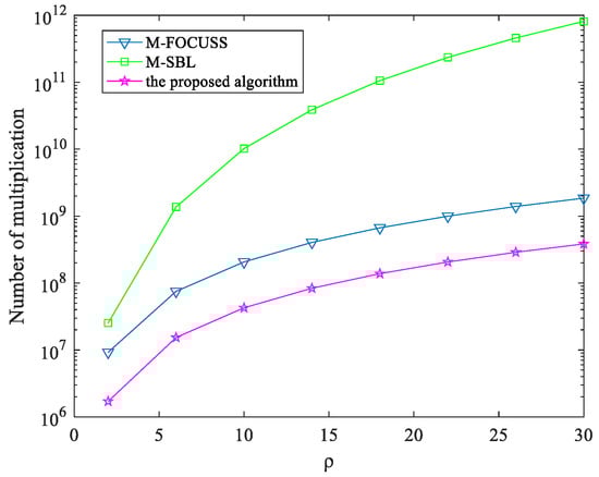
Figure 1.
Computational complexity versus for a single iteration.
5.2. Storage Analysis
In order to reflect the low storage requirement of the proposed algorithm more intuitively, we compare the proposed algorithm with the M-SBL algorithms. We need to store and in the M-SBL algorithm while we store , in the proposed algorithm. In the M-SBL algorithm, the dimension of in (12) is and the dimension of in (13) is . However, in the proposed algorithm, the dimension of in (44) is and the dimension of in (45) is . For example, when and , . In this case, the storage load in the M-SBL algorithm is heavy. Because of the sparsity of clutter, we can observe that . The storage load in the proposed algorithm is far less than the M-SBL algorithm.
5.3. Convergence Analysis
According to [], has an upper bound. We can conclude from (27) and (28) that and . has an upper bound while it is also a monotonically increasing function, which means the proposed algorithm converges.
6. Performance Assessment
In this section, we verify the performance of the proposed algorithm and the other SR-STAP algorithms with the simulated data. The parameters of the airborne radar system are listed in Table 2. The SR-STAP algorithms for comparison are the M-FOCUSS and the M-SBL. We utilize the improvement factor (IF) as the measurement of performance.
Table 2.
Parameters of airborne radar system.
6.1. Comparison of Clutter Spectrums Estimated by SR-STAP Algorithms
Clutter spectrums estimated by the proposed algorithm and other SR-STAP algorithms are compared in the absence and presence of off-grid problems. We consider three different cases: (i) A side-looking radar without off-grid problems (the platform velocity is 150 m/s and ); (ii) a side-looking radar with off-grid problems (the platform velocity is 180 m/s and ); (iii) a forward-looking radar (the platform velocity is 180 m/s). When off-grid problems occur, the effects of off-grid problems are mitigated by increasing the value of . We also set and in the M-FOCUSS and M-SBL algorithms. However, either their running time is far beyond our acceptable range, the computer crashes, or their results are wrong because of the RIP condition. Therefore, their results are not shown when and .
- (i)
- A side-looking radar without off-grid problems
We compare the high-resolution spectrum estimated by the M-FOCUSS, the M-SBL, and the proposed algorithm. In the absence of off-grid problems, the value of can be set to an integer between 2 and 5. In the experiment, . From the below figures in Figure 2, the clutter spectrums estimated by the M-SBL and the proposed algorithms are close to the ideal clutter spectrum in terms of the power and location of the clutter, which indicates the exact clutter power can be estimated by the proposed algorithm.
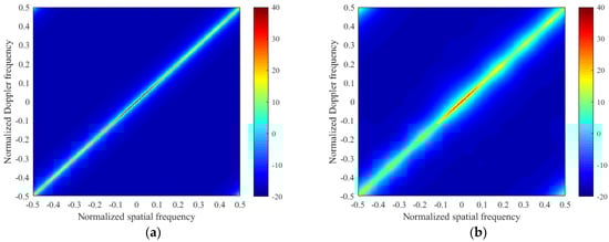
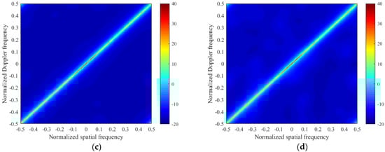
Figure 2.
Comparison between the clutter angle-Doppler spectrum estimated by different algorithms for a side-looking radar without off-grid problems. (a) Ideal clutter spectrum; (b) M-FOCUSS, ; (c) M-SBL, ; (d) the proposed algorithm, .
- (ii)
- A side-looking radar with off-grid problems
Considering that the radar is a side-looking radar with off-grid problems, we set equal to 5, 15, and 25, respectively. When or in the M-FOCUSS and M-SBL algorithms, either their running time is far beyond our acceptable range, or the computer crashes, or their results are wrong because of the RIP condition. Therefore, their results are not shown when and . From the below figures in Figure 3, the clutter spectrum estimated by the proposed algorithms is close to the ideal clutter spectrum in terms of the power and location of the clutter when , which indicates that the exact clutter power can be estimated by the proposed algorithm with sufficiently dense grids. The experiment shows that the proposed algorithm can effectively mitigate the off-grid effects.
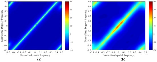
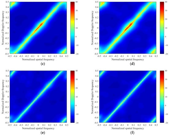
Figure 3.
Comparison between the clutter angle-Doppler spectrum estimated by different algorithms for a side-looking radar with off-grid problems. (a) Ideal clutter spectrum; (b) M-FOCUSS, ; (c) M-SBL, ; (d) the proposed algorithm, ; (e) the proposed algorithm, ; (f) the proposed algorithm, .
- (iii)
- A forward-looking radar.
Considering that the radar is a forward-looking radar, we set equal to 5, 15, and 25, respectively. From the below figures in Figure 4, the clutter spectrum estimated by the proposed algorithms is close to the ideal clutter spectrum in terms of the power and location of the clutter when , which indicates that the exact clutter power can be estimated by the proposed algorithm with sufficiently dense grids. The experiment shows that the proposed algorithm can effectively mitigate the off-grid effects.
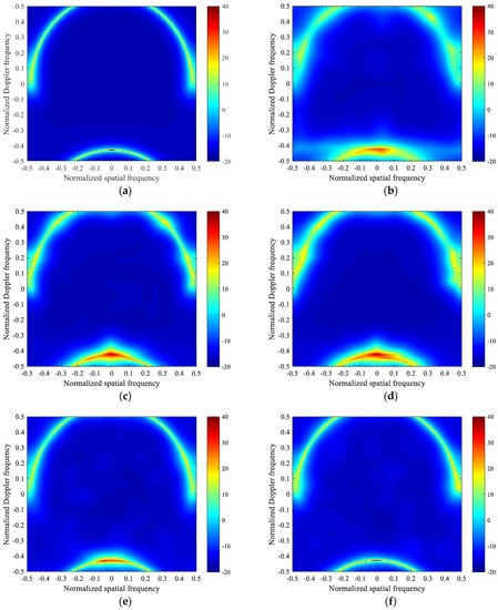
Figure 4.
Comparison between the clutter angle-Doppler spectrum estimated by different algorithms for a forward-looking radar. (a) Ideal clutter spectrum; (b) M-FOCUSS, ; (c) M-SBL, ; (d) the proposed algorithm, ; (e) the proposed algorithm, ; (f) the proposed algorithm, .
6.2. Comparison of IF Curves with SR-STAP Algorithms
In this experiment, we compare the clutter suppression performance of the proposed method with the M-FOCUSS and the M-SBL algorithms in the presence and absence of off-grid problems. Furthermore, we also consider the ideal case and the non-ideal case. Amplitude Gaussian error (standard deviation 0.03) and phase random error (standard deviation 2°) are different in all directions in the non-ideal case.
- (i)
- A side-looking radar without off-grid problems
In the absence of off-grid problems, the value of can be set equal to 5. From Figure 5, we note that the IF curves obtained by the M-SBL and the proposed algorithms are both close to the optimal IF curves obtained by the exact CNCM, which indicates that two algorithms can recover more exact clutter sources. The experiment shows that the proposed algorithm can also obtain good performance in the absence of off-grid problems.
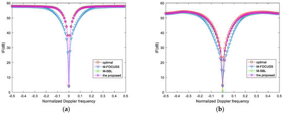
Figure 5.
IF versus normalized Doppler frequency for a side-looking radar without off-grid problems. (a) Ideal case; (b) non-ideal case with array errors.
- (ii)
- A side-looking radar with off-grid problems
Considering that the radar is a side-looking radar with off-grid problems, we set equal to 5, 15, and 25, respectively. From Figure 6, we find that increasing can effectively improve the clutter suppression performance in the presence of off-grid problems. When , the IF curves obtained by the proposed algorithm are higher and narrower than the other IF curves. The experiment shows that the proposed algorithm can effectively mitigate the off-grid effects.
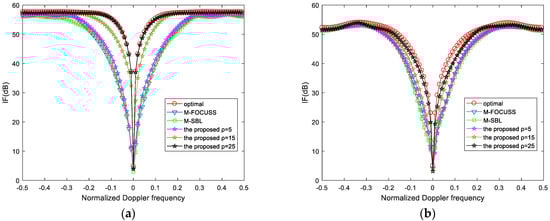
Figure 6.
IF versus normalized Doppler frequency for a side-looking radar with off-grid problems. (a) Ideal case; (b) non-ideal case with array errors.
- (iii)
- A forward-looking radar
Considering that the radar is a forward-looking radar, we set equal to 5, 15, and 25, respectively. From Figure 7, we find that increasing can effectively improve the clutter suppression performance in the presence of off-grid problems. When , the IF curves obtained by the proposed algorithm are higher and narrower than the other IF curves. The experiment shows that the proposed algorithm can effectively mitigate the off-grid effects. Theoretically, as long as the grid points are dense enough, the off-grid problems can be solved with the proposed algorithm.
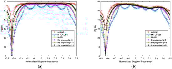
Figure 7.
IF versus normalized Doppler frequency for a forward-looking radar. (a) Ideal case; (b) non-ideal case with array errors.
6.3. Comparison of Running Time with SR-STAP Algorithms
The symbol represents the running time is far beyond our acceptable range (1 hour) or beyond the capacity of the computer. We consider three different cases: (i) A side-looking radar without off-grid problems, (ii) a side-looking radar with off-grid problems, and (iii) a forward-looking radar. The running time of the algorithm is not only affected by the convergence performance of the algorithm itself, but also the computational complexity and the burden of the storage on the computer. The computer in the simulations is equipped with Intel(R) Xeon(R) Gold 6140 CPU @ 2.30GHz 2.29GHz. The running time of the proposed algorithm in Table 3, Table 4 and Table 5 is far less than the traditional SR-STAP algorithms, especially when dense grids are exploited. One hundred Monte Carlo trials were performed to obtain the average running time.
- (i)
- A side-looking radar without off-grid problems
Table 3.
Running time of different algorithms for a side-looking radar without off-grid problems.
Table 3.
Running time of different algorithms for a side-looking radar without off-grid problems.
| Algorithm | The Average Running Time (s) |
|---|---|
| M-FOCUSS | 1.05 |
| M-SBL | 26.32 |
| the proposed algorithm | 0.88 |
- (ii)
- A side-looking radar with off-grid problems
Table 4.
Running time of different algorithms for a side-looking radar with off-grid problems.
Table 4.
Running time of different algorithms for a side-looking radar with off-grid problems.
| Algorithm | The Average Running Time (s) | ||
|---|---|---|---|
| M-FOCUSS | 1.13 | 72.23 | |
| M-SBL | 29.79 | ||
| the proposed algorithm | 1.06 | 3.36 | 12.14 |
- (iii)
- A forward-looking radar
Table 5.
Running time of different algorithms for a forward-looking radar.
Table 5.
Running time of different algorithms for a forward-looking radar.
| Algorithm | The Average Running Time (s) | ||
|---|---|---|---|
| M-FOCUSS | 1.02 | 64.14 | |
| M-SBL | 30.62 | ||
| the proposed algorithm | 1.05 | 4.03 | 12.94 |
7. Conclusions
A novel SR-STAP algorithm is proposed to mitigate off-grid effects. The proposed algorithm is based on the Bayes criterion and mitigates off-grid effects when the grid interval is sufficiently small. We pick out which atoms are in the subspace of clutter, which means the proposed algorithm does not need to satisfy the restricted isometry property (RIP) condition. Moreover, the complexity and storage requirement of the proposed algorithm is low, and its convergence can be promised.
Author Contributions
Conceptualization, T.W.; methodology, C.L.; validation, C.L., K.L. and X.Z.; writing—original draft preparation, C.L.; writing—review and editing, K.L. and X.Z.; visualization, C.L., K.L. and X.Z.; supervision, T.W.; project administration, T.W. All authors have read and agreed to the published version of the manuscript.
Funding
This research was funded by the National Key R&D Program of China, grant number 2021YFA1000400.
Data Availability Statement
In this section, please provide details regarding where data supporting reported results can be found, including links to publicly archived datasets analyzed or generated during the study. Please refer to suggested Data Availability Statements in section “MDPI Research Data Policies” at https://www.mdpi.com/ethics. You might choose to exclude this statement if the study did not report any data.
Conflicts of Interest
The authors declare no conflict of interest.
Appendix A
In order to make the following formulas more intuitive and concise, we remove from quantities in the -th iteration, and updated quantities in the -th iteration are denoted by a tilde (). As stated in the text, represents the serial number of the hyper-parameter that needs to be updated in the -th iteration. also represents the position index of in . When is already in , is defined as the position index of in .
- When ,where and .
- When ,where , and .
- When ,
References
- Ward, J. Space-Time Adaptive Processing for Airborne Radar; Technical Report; MIT Lincoln Laboratory: Lexington, KY, USA, 1998. [Google Scholar]
- Reed, I.S.; Mallet, J.D.; Brennan, L.E. Rapid convergence rate in adaptive arrays. IEEE Trans. Aerosp. Electron. Syst. 1974, 10, 853–863. [Google Scholar] [CrossRef]
- Donoho, D.L.; Elad, M.; Temlyakov, V.N. Stable recovery of sparse overcomplete representations in the presence of noise. IEEE Trans. Inf. Theory 2006, 52, 6–18. [Google Scholar] [CrossRef]
- Sun, K.; Zhang, H.; Li, G.; Meng, H.D.; Wang, X.Q. A novel STAP algorithm using sparse recovery technique. IEEE Int. Geosci. Remote Sens. Symp. 2009, 1, 3761–3764. [Google Scholar]
- Yang, Z.C.; Li, X.; Wang, H.Q.; Jiang, W.D. On clutter sparsity analysis in space-time adaptive processing airborne radar. IEEE Geosci. Remote Sens. Lett. 2013, 10, 1214–1218. [Google Scholar] [CrossRef]
- Sen, S. Low-rank matrix decomposition and spatial-temporal sparse recovery for STAP radar. IEEE J. Sel. Top. Signal Process. 2015, 9, 1510–1523. [Google Scholar] [CrossRef]
- Yang, Z.; Wang, Z.; Liu, W.; de Lamare, R.C. Reduced-dimension space-time adaptive processing with sparse constraints on beam-Doppler selection. Signal Process. 2019, 157, 78–87. [Google Scholar] [CrossRef]
- Zhang, W.; An, R.; He, N.; He, Z.; Li, H. Reduced dimension STAP based on sparse recovery in heterogeneous clutter environments. IEEE Trans. Aerosp. Electron. Syst. 2019, 56, 785–795. [Google Scholar] [CrossRef]
- Liu, C.; Wang, T.; Zhang, S.G.; Ren, B. Clutter suppression based on iterative reweighted methods with multiple measurement vectors for airborne radar. IET Radar Sonar Navig. 2022, 16, 1–14. [Google Scholar] [CrossRef]
- Candes, M.; Wakin, M.; Boyd, S. Enhancing sparsity by reweighted minimization. J. Fourier Anal. Appl. 2008, 5, 877–905. [Google Scholar] [CrossRef]
- Tipping, M.E. Sparse Bayesian learning and the relevance vector machine. J. Mach. Learn. 2001, 1, 211–244. [Google Scholar]
- Wipf, D.P.; Rao, B.D. Sparse Bayesian learning for basis selection. IEEE Trans. Signal Process. 2004, 52, 2153–2164. [Google Scholar] [CrossRef]
- Wipf, D.P.; Rao, B.D. An empirical Bayesian strategy for solving the simultaneous sparse approximation problem. IEEE Trans. Signal Process. 2007, 55, 3704–3716. [Google Scholar] [CrossRef]
- Tipping, M.E.; Faul, A.C. Fast marginal likelihood maximization for sparse Bayesian models. In Proceedings of the Ninth International Workshop on Artificial Intelligence and Statistics, Key West, FL, USA, 3–6 January 2003; Volume 1, pp. 276–283. [Google Scholar]
- Ji, S.H.; Xue, Y.; Carin, L. Bayesian compressive sensing. IEEE Trans. Signal Process. 2008, 56, 2346–2356. [Google Scholar] [CrossRef]
- Ji, S.H.; Dunson, D.; Carin, L. Multi-task compressive sensing. IEEE Trans. Signal Process. 2009, 57, 92–106. [Google Scholar] [CrossRef]
- Babacan, S.D.; Molina, R.; Katsaggelos, A.K. Bayesian compressive sensing using Laplace priors. IEEE Trans. Image Process. 2010, 19, 53–63. [Google Scholar] [CrossRef]
- Wu, Q.S.; Zhang, Y.M.; Amin, M.G.; Himed, B. Complex multitask Bayesian compressive sensing. In Proceedings of the 2014 IEEE International Conference on Acoustics, Speech and Signal Processing (ICASSP), Florence, Italy, 4–9 May 2014. [Google Scholar]
- Serra, J.G.; Testa, M.; Katsaggelos, A.K. Bayesian K-SVD using fast variational inference. IEEE Trans. Image Process. 2017, 26, 3344–3359. [Google Scholar] [CrossRef]
- Ma, Z.Q.; Dai, W.; Liu, Y.M.; Wang, X.Q. Group sparse Bayesian learning via exact and fast marginal likelihood maximization. IEEE Trans. Signal Process. 2017, 65, 2741–2753. [Google Scholar] [CrossRef]
- Liu, C.; Wang, T.; Zhang, S.G.; Ren, B. A fast space-time adaptive processing algorithm based on sparse Bayesian learning for airborne radar. Sensors 2022, 22, 2664. [Google Scholar] [CrossRef]
- Duan, K.Q.; Wang, Z.T.; Xie, W.C.; Chen, H.; Wang, Y.L. Sparsity-based STAP algorithm with multiple measurement vectors via sparse Bayesian learning strategy for airborne radar. IET Signal Process. 2017, 11, 544–553. [Google Scholar] [CrossRef]
- Wang, Z.T.; Xie, W.C.; Duan, K.Q. Clutter suppression algorithm base on fast converging sparse Bayesian learning for airborne radar. Signal Process. 2017, 130, 159–168. [Google Scholar] [CrossRef]
- Yang, X.P.; Sun, Y.Z.; Yang, J.; Long, T.; Sarkar, T.K. Discrete Interference suppression method based on robust sparse Bayesian learning for STAP. IEEE Access 2019, 10, 26740–26751. [Google Scholar] [CrossRef]
- Duan, K.Q.; Liu, W.J.; Duan, G.Q.; Wang, Y.L. Off-grid effects mitigation exploiting knowledge of the clutter ridge for sparse recovery STAP. IET Radar Sonar Navig. 2018, 12, 557–564. [Google Scholar] [CrossRef]
- You, K.T.; Guo, W.B.; Liu, Y.L.; Wang, W.B.; Sun, Z. Grid evolution: Joint dictionary learning and sparse Bayesian recovery for multiple off-grid targets localization. IEEE Commun. Lett. 2018, 22, 2068–2071. [Google Scholar] [CrossRef]
- Dai, J.S.; Bao, X.; Xu, W.C.; Chang, C.Q. Root sparse Bayesian learning for off-grid DOA estimation. IEEE Signal Process. Lett. 2017, 24, 46–50. [Google Scholar] [CrossRef]
- Fang, J.; Wang, F.Y.; Shen, Y.N.; Li, H.B.; Blum, R.S. Super-resolution compressed sensing for line spectral estimation: An iterative reweighted approach. IEEE Trans. Signal Process. 2016, 64, 4649–4662. [Google Scholar] [CrossRef]
- Fang, J.; Shen, Y.N.; Li, H.B.; Li, S.Q. Super-resolution compressed sensing: An iterative reweighted algorithm for joint parameter learning and sparse signal recovery. IEEE Signal Process. Lett. 2014, 21, 761–766. [Google Scholar]
- Li, Z.H.; Zhang, Y.S.; He, X.Y.; Guo, Y.D. Low-complexity off-grid STAP algorithm based on local search clutter subspace estimation. IEEE Geosci. Remote Sens. Lett. 2018, 15, 1862–1865. [Google Scholar] [CrossRef]
- Yuan, H.D.; Xu, H.; Duan, K.Q.; Xie, W.C.; Liu, W.J.; Wang, Y.L. Sparse Bayesian learning-based space-time adaptive processing with off-grid self-calibration for airborne radar. IEEE Access 2018, 6, 47296–47307. [Google Scholar] [CrossRef]
- Wipf, D.; Nagarajan, S. A new view of automatic relevance determination. In Advances in Neural Information Processing Systems 20; MIT Press: New York, NY, USA, 2008. [Google Scholar]
Publisher’s Note: MDPI stays neutral with regard to jurisdictional claims in published maps and institutional affiliations. |
© 2022 by the authors. Licensee MDPI, Basel, Switzerland. This article is an open access article distributed under the terms and conditions of the Creative Commons Attribution (CC BY) license (https://creativecommons.org/licenses/by/4.0/).