Susceptibility Analysis of Land Subsidence along the Transmission Line in the Salt Lake Area Based on Remote Sensing Interpretation

Abstract

As the influence of extreme climate and human engineering activities intensifies, land subsidence frequently occurs in the Salt Lake area of Qinghai Province, China, which seriously threatens the stability of the UHV transmission line crossing the area. Current susceptibility analyses of land subsidence disasters have mostly focused on the classification of land subsidence susceptibility and have ignored the differentiation of susceptibility among different land subsidence intensities. Therefore, the land subsidence susceptibility map does not meet the operation and maintenance management needs of the UHV transmission line, let alone planning and designing of new lines in the Salt Lake area. Therefore, in this study, we proposed a susceptibility analysis of different land subsidence intensities along the transmission line in the Salt Lake area. The small baseline integrated aperture radar interferometry (SBAS-InSAR) method was used to obtain the land subsidence along the transmission line based on 67 Sentinel-1 remote sensing interpretation datasets from 2017 to 2021. Based on a combination of K-means clustering and the transmission line specifications, four annual land subsidence intensity grades were identified as 0~−2 mm/year, −2~−10 mm/year, −10~−20 mm/year, and <−20 mm/year. In addition, eight geological environmental factors were analyzed, and a multi-layer perceptron neural network (MLPNN) model was used to calculate the susceptibility of the different land subsidence intensities. The area under the curve (AUC) and practical examples were used to verify the reliability of the different land subsidence intensities susceptibility mapping. The AUC values of the four subsidence intensity grades showed that the results were accurate: the <−20 mm/year grade produced the largest AUC (0.951), with the −10~−20 mm/year, −2~−10 mm/year and 0~−2 mm/year grades producing AUCs of 0.926, 0.812, 0.879, respectively. At the same time, the susceptibility classification results of different land subsidence intensities were consistent with the interpretation and site tower deformation. The results of this study provided the distribution of land subsidence susceptibility along the transmission line, distinguished the susceptibility of different land subsidence intensities, and provided more detailed subsidence information for each transmission tower. The results provide important information for transmission line tower planning, design, protection, and operation management.

1. Introduction

With the rapid development of the western part of China and the “One Belt One Road” strategy, a 750 kV transmission line in the Qaidam Basin of Qinghai Province shoulders the responsibility for western energy transportation. When transmission lines pass through a complex geological environment, the relationship between tower deformation and surrounding environmental factors must be considered, including the unique geological conditions in the Salt Lake area [1,2]. However, due to climate change and human engineering activities, saline soil is prone to collapse as a bearing layer [3]. Thus, some transmission towers constructed in the Salt Lake area are threatened by different grades of land subsidence intensities, and some have already failed [2,4]. Land subsidence is a gradual deformation or sudden collapse of the Earth’s surface caused by numerous natural and human-induced factors [5,6,7], which seriously threaten the stability of infrastructure, power lines, and buildings [8,9,10,11]. Due to the wide distribution of saline soil along the UHV transmission line in the Salt Lake area, the soil is prone to uplifting and collapsing deformation under the action of external factors [12], and the resulting land subsidence seriously threatens the safety and stability of the transmission line towers. The operation of these transmission towers faces significant challenges [2,13]. Therefore, to monitor and avoid failure of the UHV transmission towers in this specific area and to guide the planning, design, protection, and operations management of new transmission towers, it is important to determine the land subsidence distribution and intensities along the UHV transmission line.

UHV transmission lines usually traverse long distances. As compared with the traditional geodetic and GPS measurement methods [14,15], the satellite-based synthetic aperture radar (SAR) monitoring method can meet the accuracy of the surface deformation monitoring demand along the lines and also has a broader coverage area and higher cost benefits [16,17,18]. A long-term InSAR method is usually used to obtain the time-series analysis results by interpreting the permanent scatterers in the InSAR datasets [19]. The long-term InSAR time-series method has been widely used to analyze the deformation and displacement of geological calamities, such as landslides [20,21,22] and land subsidence [23,24,25,26,27]. Because saline soil is widely distributed in the study area, the deformation of saline soil, such as salt swelling and collapsibility, may lead to the destruction of soil structure [28,29]. Therefore, monitoring the deformation and failure of transmission towers caused by the saline soil is necessary [2]. Land subsidence along UHV transmission lines can be quickly and effectively obtained by using the more accurate SBAS-InSAR method and Sentinel-1 datasets from ESA [30,31,32]. Due to the different geological environments of UHV transmission lines, the intensities of the land subsidence are different along the lines [33]. Different intensities of land subsidence have required different disaster prevention plans [34,35]. To date, some studies have been carried out to obtain land subsidence intensities and subsidence intensity classification based on some specific research areas [34,36], and some Chinese specifications [37,38,39] have also suggested the threshold of land subsidence in the power sector, however, these specifications do not apply to the classification of land subsidence intensities of transmission line towers in the Salt Lake area. In addition, the intensity classification method and standards of those land subsidence intensities were not united, and therefore, the classification results have not contributed to susceptibility mapping. At present, there are different classification methods in the classification of land subsidence intensity. Some are classified according to different economic distributions in the study area, and others are classified according to the intensity and clustering of land subsidence [34,35]. In the classification of land subsidence intensity and clustering, due to K-means method can cluster and analyze the data, which is extensively applied in the analysis of the land subsidence results by remote sensing interpretation [40]. In Jixi, China, the K-means method was used to class the evaluation results of remote sensing images and then distinguish the land subsidence intensity [41]. In Chapai Nawabgonj, Bangladesh, the K-means method was applied to better understand the subsidence rate in the area after using the Sentinel-1 satellite to obtain surface deformation data [42]. However, the use of the K-means method above mostly stays in the distribution of land subsidence intensity, and there is still a lack of further research on different land subsidence intensity grades.

The machine learning algorithm provides a fast and accurate method for land subsidence susceptibility mapping [43,44,45,46]. Artificial neural network [47], decision tree [48], random forest [49], support vector machine [50], and other machine learning methods [51,52] have been widely used and have achieved excellent evaluation results. MLPNN, as a machine learning algorithm with excellent performance, is widely used in the study of land subsidence susceptibility, such as Jakarta, Seoul, etc. [8,47,50]. At the same time, in the Qarhan Salt Lake area of China, the results of land subsidence susceptibility were obtained by combining the remote sensing interpretation with the machine learning algorithm and found that the MLPNN is more suitable for the modeling of land subsidence susceptibility in the Salt Lake area [53]. According to the above research, the susceptibility modeling of land subsidence mainly focuses on subsidence, but the susceptibility modeling of different land subsidence intensities has not been considered.

In this study, we used the Sentinel-1 satellite datasets and the SBAS-InSAR meth-od to obtain the ground deformation along the UHV transmission line that crosses the Qarhan Salt Lake area in Qinghai Province, China. The deformation time-series diagram of a typical transmission tower was generated according to the vertical deformation. Based on the relevant specifications of electric power and the K-means clustering method, the land subsidence intensities along the UHV transmission line were classified. Then, the land subsidence susceptibility map for different land subsidence intensities was generated using the training and test datasets divided by the MLPNN. The receiver operating characteristic (ROC) and area under the curve (AUC) were used to evaluate the performance of the model and the reliability of the land subsidence susceptibility mapping. By using K-means clustering to distinguish the interpretation results of different intensities and susceptibility mapping, we proposed a new method for the study of land subsidence. At the same time, by combining remote sensing interpretation, the K-means clustering method, and a machine learning algorithm, in this study, we obtained the distribution of land subsidence susceptibility along the transmission line, distinguished the susceptibility of different land subsidence intensities, and provided more detailed subsidence information for each transmission tower. The results enhance the understanding of varying land subsidence intensity prone areas and provide important information for transmission line tower planning, design, protection, and operations management.

2. Materials and Methods

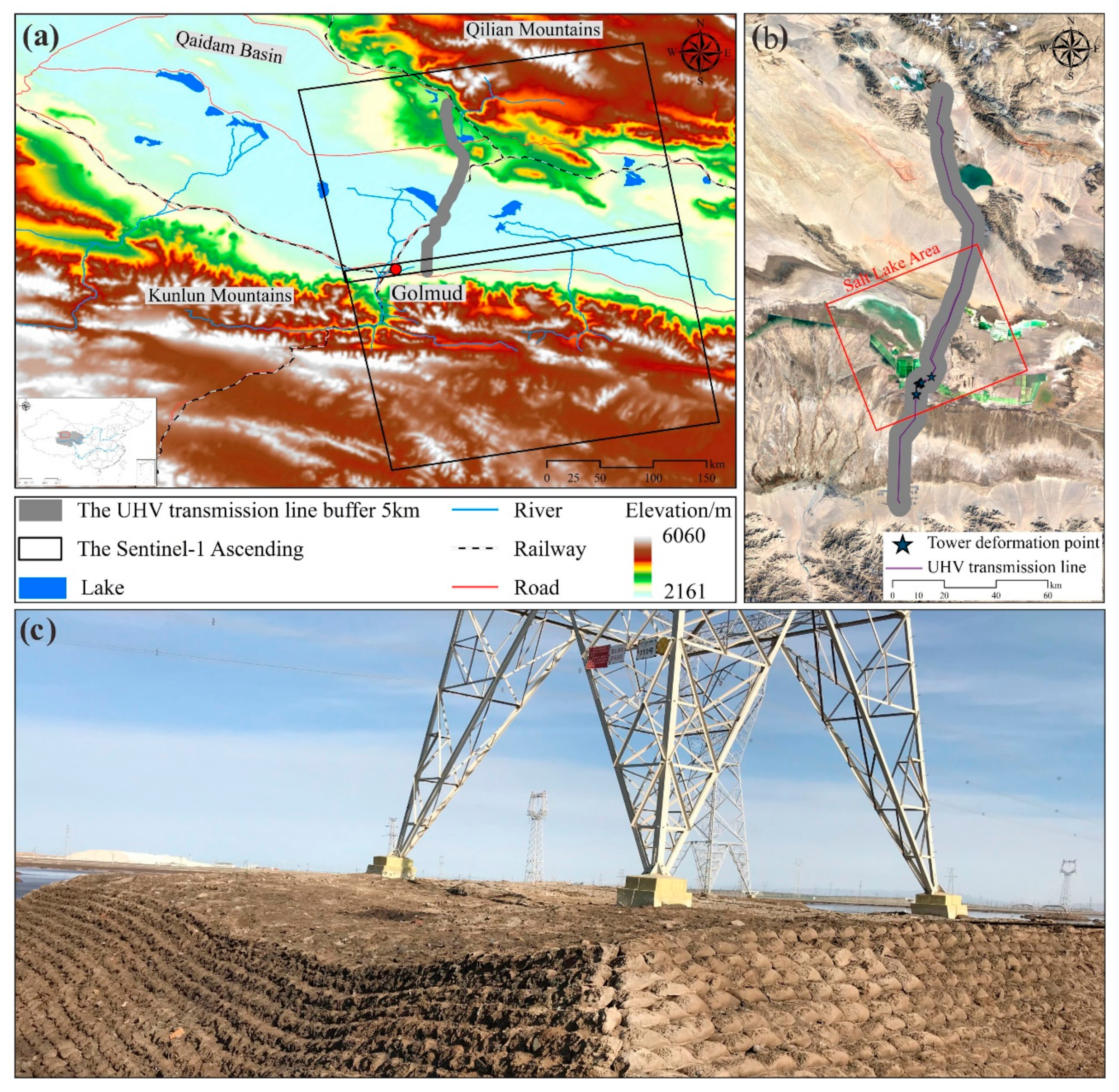
2.1. Study Areas

In this study, the UHV transmission line studied traverses the Qarhan Salt Lake area in Qinghai Province, China, from north to south. The total length of the line is about 170 km, and nearly half of the line towers are located in the central Qarhan Salt Lake area. The Qarhan Salt Lake is located in the center of the southern Qaidam Basin of northwestern China. Because the lake develops at the lowest point, it gathers water throughout the basin, leading to the deposition of thick lacustrine and fluvial sediments [54]. The Qilian Mountains are located in the northeast of Salt Lake, and the Kunlun Mountains are located in the south. Affected by high mountain snowmelt, the seasonal rivers along the transmission line are widely developed. The UHV transmission line is located in the plateau desert climate, and the weather is dry and rainless all year. According to data from the city of Golmud near the transmission line, the average precipitation is only 43 mm/year, and the potential evaporation capacity is as high as 2430 mm/year [55]. Under the effect of strong evaporation, the mineral salt crystals in the Qarhan Salt Lake precipitate to form an arid saline mudflat [33]. To facilitate transportation, the Qinghai–Tibet Railway and highway cross the dry salt mud beach in the middle of the Salt Lake area. Quaternary sediments are widely distributed along the UHV transmission line. The quaternary chemical sediments in the Salt Lake area pro-vide abundant material sources to exploit mineral salts [56]. However, the continuous mining of mineral salt has caused the water level of the underground aquifer to decline, resulting in changes in the stress of the upper salt layer and causing ground deformation [33].

According to the field survey results, most of the transmission towers across the Salt Lake area have been deformed. The most severe deformation tower is shown in Figure 1b.

2.2. SAR Datasets

The land subsidence results along the transmission line were obtained from Sentinel-1A SAR C-band data provided by the European Space Agency (ESA) (Supplementary Materials: Sentinel-1 Satellite Dataset). Sentinel-1A has an acquisition cycle of 12 days. The SAR images can be interpreted to map the surface deformation over a large area, and the ground deformation in different periods can be obtained simultaneously. This study collected 67 SAR scenes from April 2017 to May 2021, which are listed in

Table 1. The reference date shown in bold text shows the acquisition dates of data from the Sentinel-1 satellite in descending tracks. Delta days = number of days between each acquisition date. B⊥ = perpendicular baseline.

No.	Acquisition Date (yyyy/mm/dd)	Days	B⊥(m)	No.	Acquisition Date (yyyy/mm/dd)	Days	B⊥(m)	No.	Acquisition Date (yyyy/mm/dd)	Days	B⊥(m)
1	2017/4/28	−360	73	24	2018/7/4	72	83	47	2019/9/21	516	−55
2	2017/5/22	−336	27	25	2018/7/16	84	32	48	2019/10/15	540	90
3	2017/6/15	−312	12	26	2018/7/28	96	75	49	2019/11/20	576	−41
4	2017/7/21	−276	63	27	2018/8/9	108	71	50	2019/12/26	612	95
5	2017/8/26	−240	12	28	2018/8/21	120	−10	51	2020/1/7	624	88
6	2017/9/19	−216	46	29	2018/9/2	132	−78	52	2020/2/12	660	23
7	2017/10/25	−180	−40	30	2018/9/14	144	14	53	2020/3/7	684	21
8	2017/11/30	−144	75	31	2018/9/26	156	59	54	2020/4/12	720	−30
9	2017/12/24	−120	81	32	2018/10/8	168	89	55	2020/5/6	744	99
10	2018/1/5	−108	78	33	2018/10/20	180	−3	56	2020/6/11	780	23
11	2018/1/17	−96	95	34	2018/11/1	192	−35	57	2020/7/5	804	123
12	2018/1/29	−84	97	35	2018/11/13	204	7	58	2020/8/10	840	−65
13	2018/2/10	−72	19	36	2018/11/25	216	96	59	2020/9/3	864	91
14	2018/2/22	−60	8	37	2018/12/7	228	61	60	2020/10/9	900	−118
15	2018/3/6	−48	19	38	2018/12/31	252	27	61	2020/11/2	924	71
16	2018/3/18	−36	69	39	2019/1/12	264	9	62	2020/12/8	960	−6
17	2018/3/30	−24	72	40	2019/2/17	300	70	63	2021/1/1	984	54
18	2018/4/23	0	0	41	2019/3/13	324	−19	64	2021/2/6	1020	39
19	2018/5/5	12	37	42	2019/4/6	348	23	65	2021/3/14	1056	55
20	2018/5/17	24	37	43	2019/5/12	384	−9	66	2021/4/7	1080	26
21	2018/5/29	36	48	44	2019/6/17	420	95	67	2021/5/1	1104	99
22	2018/6/10	48	8	45	2019/7/11	444	18
23	2018/6/22	60	7	46	2019/8/16	480	34

. The reference datasets with zero delta day and zero perpendicular baselines from the ascending track, on 23 April 2018 as the reference date, are shown in bold text.

2.3. Land Subsidence Eveluation Index

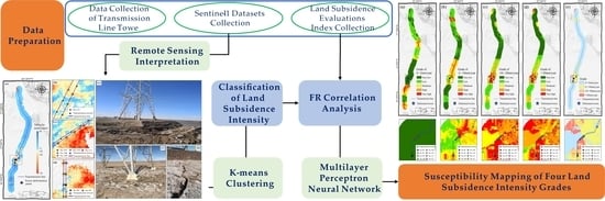
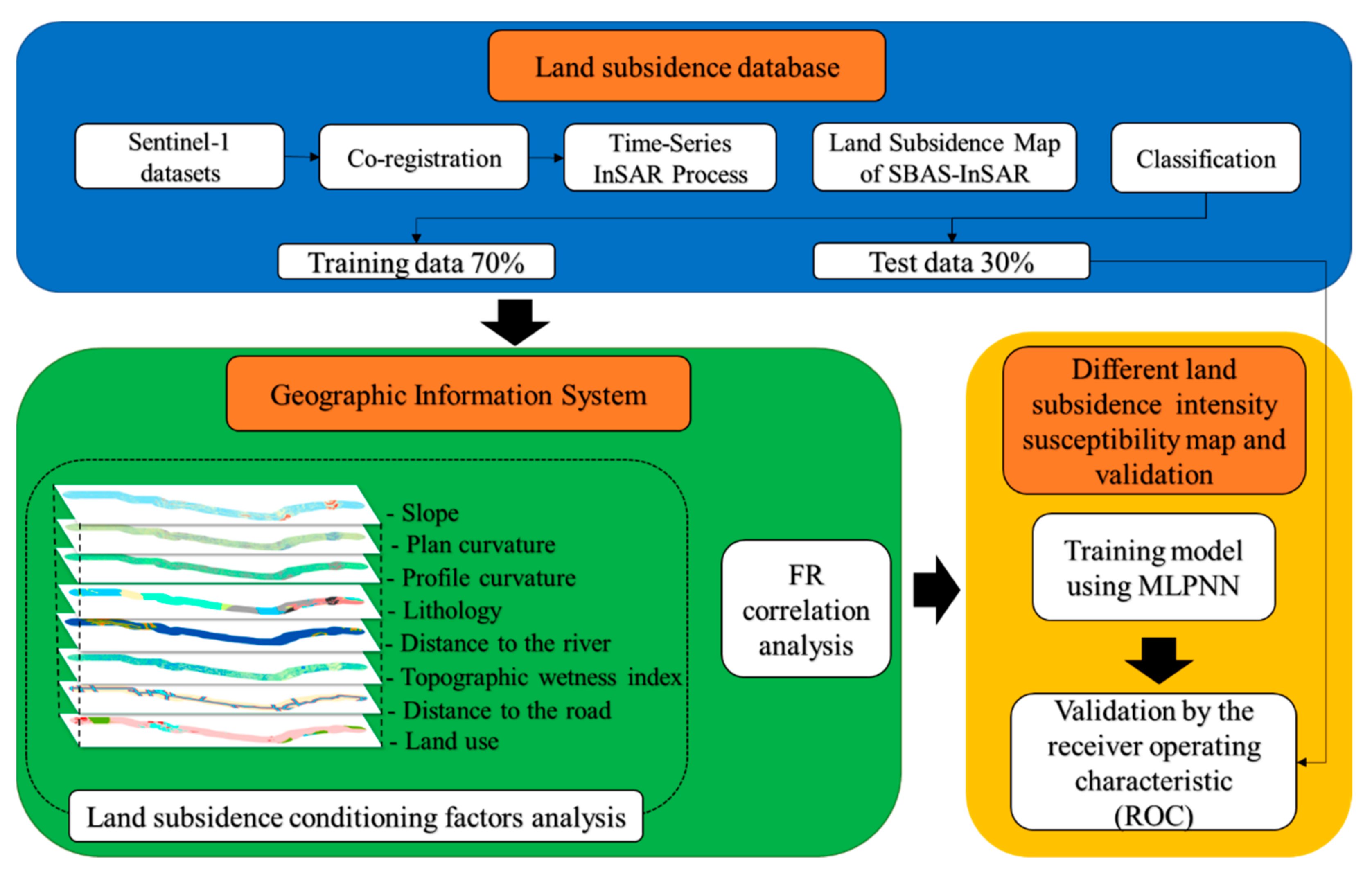
According to a survey of the geological calamity along the UHV transmission line, the main influencing factors of land subsidence in the Salt Lake area include hydrogeology, human activities, engineering geological characteristics of saline soil, and external environmental factors [8,33,51,52,57,58,59,60,61]. Eight conditioning factors were considered for the analysis, including topography, geology, hydrology, and human engineering activities. After obtaining various conditioning factors, they were standardized and resampled into raster datasets with 40 m cell size. The classification scheme for each conditioning factor is shown in

Table 2. Land subsidence factors and sources along transmission lines in the Salt Lake area.

Category	Factor	Source	Data Form	Data Scale
Topography	Slop	DEM SRTM from the Geospatial Data Cloud platform	Raster	30 m
	Plan curvature	DEM SRTM from the Geospatial Data Cloud platform	Raster	30 m
	Profile curvature	DEM SRTM from the Geospatial Data Cloud platform	Raster	30 m
Geology	Lithology	National Geological Archives of China	Vector	1:50,000
Hydrology	Distance to River	Geospatial Data Cloud platform	Vector	1:100,000
	Topographic Wetness Index (TWI)	DEM SRTM from the Geospatial Data Cloud platform	Raster	30 m
Human engineering activity	Distance to Road	Geospatial Data Cloud platform	Vector	1:100,000
	Land use	Institute of Tibetan Plateau Research, Chinese Academy of Sciences	Raster	30 m

.

In this study, we extracted topography datasets from the SRTM DEM from the Geospatial Data Cloud platform, slope, plan curvature, profile curvature, and TWI by GIS (Figure 2a–c,f). The slope affects water flow velocity; the plan curvature reflects the directional variations along a curve [62]; the profile curvature represents the amount of elevation variation along the flow path [63]; and the TWI defines the degree of water deposition at a specific site [64], which all significantly influence the flow direction and accumulation of surface water, indirectly leading to land subsidence [45,51,52,65].

Lithology provides internal development conditions for the occurrence of various geological disasters and makes a vital contribution to the development of land subsidence. According to the National Geological Archives of China’s 1:250,000 geological maps of the study area, the Quaternary sediments along the UHV transmission line are widely distributed, and the Quaternary chemical sediments are the most exposed (Figure 2d).

Surface water and groundwater in the study area mainly originate from precipitation and snowmelt in the mountainous areas (Figure 2e) [66]. Therefore, the surface rivers and groundwater levels show a seasonal change trend, which may affect salty soil stability and increase the possibility of land subsidence [33].

The Qinghai–Tibet Railway and highway cross the Salt Lake area, coupled with dense transport corridors near the saltern area (Figure 2g). Therefore, vehicle loads frequently change soil structure stability and cause foundation instability [12]. The land-use map (Figure 2h) was obtained from the Institute of Tibetan Plateau Research at the Chinese Academy of Sciences. From the map, we can see that most land use is bare, and the saltern area is located in the center of the UHV transmission line.

2.4. Methodology

The workflow of the MLPNN to generate the susceptibility map of different land subsidence intensities along the UHV transmission line is shown in Figure 3. The methods are summarized as follows:

• Land subsidence database.

Land subsidence occurrences were identified by exploiting Sentinel-1 SAR datasets from 2017 to 2021 using time-series InSAR based on the SBAS-InSAR method. The persistent scatterer points showing a deformation value were used as the land subsidence inventory map. After obtaining the land subsidence inventory map, the K-means clustering method was used to divide the land subsidence inventory map into different land subsidence intensities. Then, the land subsidence susceptibility model randomly divided the vertical deformation subsidence points with different land subsidence intensities into 70% training data. The land subsidence susceptibility map was verified by using 30% of the test data.

2.

Geographic information system.

Aimed at the characteristics of the study area and selected the influencing factors of land subsidence. Then, the frequency ratio method was used to analyze the conditioning factors and identify the correlations among various factors and different land subsidence intensities.

3.

Land subsidence intensity susceptibility map and validation.

MLPNN was used to generate the land subsidence susceptibility map with different land subsidence intensities, and the ROC curves were used for validation after generating the land subsidence susceptibility map under different land subsidence intensities.

2.5. Time-Series InSAR Process

The UHV transmission line is located in the arid and saline desert area of the Qarhan Basin, China. Vegetation cover along the lines is sparse, primarily bare sandy or saline soil, and therefore, as compared with most areas in China, the interference coherence is relatively high in a short time. Under a limited time-series baseline condition, high-quality interference pairs can be obtained, and then a tiny baseline grid with high interference coherence can be formed [33]. To obtain more accurate land subsidence intensities along the transmission line, in this study, we adopted the SBAS-InSAR method to make use of coherent targets (CTs) with high coherence. We used weighted least squares (WLS) estimation to obtain the high precision time-series deformation results of the CTs [54,55]. In the process of SBAS-InSAR, one of the N+1 SAR images was selected as the primary image of registration at first, and M interferograms that meet the spatiotemporal baseline threshold were selected. The interference phase of each interferogram is composed of multiple phase components, as follows:

$$\delta {\phi }_{x,\alpha }={\phi }_{x,\alpha }\left(t_B\right)-{\phi }_{x,\alpha }\left(t_A\right)\approx \delta {\phi }_{x,\alpha }{}^{def}+\delta {\phi }_{x,\alpha }{}^{topo}+\delta {\phi }_{x,\alpha }{}^{atm}+\delta {\phi }_{x,\alpha }{}^{noise}$$

(1)

where ${\phi }_{x,\alpha }\left(t_B\right)$ and ${\phi }_{x,\alpha }\left(t_A\right)$ represent phase values of SAR images at $t_A$ and $t_B$, respectively; $\delta {\phi }_{x,\alpha }{}^{def}$ refers to the deformation phase between times $t_A$ and $t_B$; $\delta {\phi }_{x,\alpha }{}^{topo}$ corresponds to the residual phase due to inaccuracies in reference DEM. $\delta {\phi }_{x,\alpha }{}^{atm}$ depicts the atmospheric phase error; $\delta {\phi }_{x,\alpha }{}^{noise}$ denotes the random noise phases.

The deformation velocity ($d_{LOS}$) of different SAR acquisition times can be obtained by 3D Spatiotemporal phase unwrapping of M interferograms. In this study, we mainly considered the deformation of transmission towers caused by the vertical deformation of the ground. Assuming that the horizontal deformation is small relative to the vertical deformation caused by land subsidence, the deformation map obtained from the line of sight (LOS) displacement can be converted into the vertical deformation data [56,57,58,59].

$$d_V=\frac{d_{LOS}}{\cos \theta }$$

(2)

where $d_V$ represents the vertical deformation, $d_{LOS}$ represents the deformation from the line of sight, and $\theta$ is the cosine of the incident angle from the radar signal.

2.6. Land Subsidence Intensity Classification Based on the K-Means Method

The K-means method divides the data into several homogeneous clusters with similar features, initializes the center of the K-cluster by random search in each iteration, and then measures the distance between the data point ($x_{ij}$) and the center ($c_j$). By minimizing the objective function specified by Equation (1), cluster k is assigned to the data point $x_{ij}$ [60].

$$Minimize:d={\displaystyle \sum }_{j=1}^k.{\displaystyle \sum }_{i=1}^k.\Vert x_{ij}-c_j{}^2\Vert$$

(3)

2.7. FR Correlation Analysis

The frequency ratio (FR) method was used to analyze the spatial correlation of land subsidence conditioning factors with different land subsidence intensities [52]. Combined with the above deformation distribution of the towers, −10~−20 mm/year, −2~−10 mm/year and <−20 mm/year were the primary analysis objectives.

$$FR=\frac{Area ratio of land subsidence velocity}{area ratio of class conditioning factor }$$

(4)

The FR index represents the importance of conditioning factors associated with the occurrence of different land subsidence intensities. An FR value of >1 indicates that the conditioning factor is conducive to the event of this intensity of land subsidence intensities. An FR value of <1 indicates that the conditioning factor is not conducive to this intensity of land subsidence intensities [67,68].

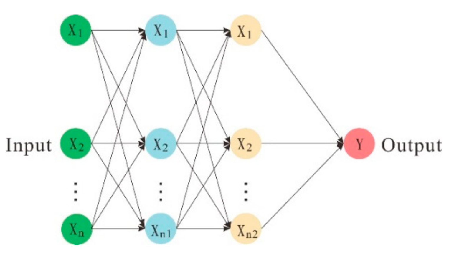
2.8. Multi-Layer Perceptron Neural Network

The multi-layer perceptron neural network model (MLPNN) is a forward-oriented layered structure. It mainly comprises the input layer, the output layer, and the hidden layer (Figure 4) [69]. It maps the input data to the output through training and learning, thus forming the MLPNN model. Finally, the neural network establishes the most suitable fitting model according to the input sample data, and the parameters are set to ensure that this model can be applied to other similar data.

In this study, according to the above classification of different land subsidence intensities along the UHV transmission line, when the land subsidence intensity value of a certain grade was set to 1 for analysis, the residual intensity value was set to 0. Finally, the whole model dataset was randomly separated into the training dataset (70%) and the test dataset (30%). The modeling process was implemented using the SPSS Modeler software (Machines Corporation, Armonk, NY, USA).

3. Results

3.1. Land Subsidence Map of SBAS-InSAR

According to the SBAS-InSAR method, we obtained the results of deformation velocity in the study area, as shown in Figure 5a. The land subsidence along the UHV transmission line mainly occurs in the central Salt Lake area. This is consistent with the actual distribution of transmission tower deformation and failure. The remaining land subsidence areas mainly occur near rivers and lakes, which may be related to seasonal alpine snowmelt.

To analyze the time-series deformation of the UHV transmission line towers, the average vertical deformation maps of damaged transmission line towers, including No. 98, No. 99, No. 107, No. 108, No. 109, No. 110, No. 111, and No. 121, are overlaid, as shown in Figure 5b–d. From Figure 5b–d, it can be seen that the towers that have undergone deformation and failure are located in the serious deformation areas along the whole transmission line. According to the field survey in Figure 5e–g, it can be seen that the towers’ structures and foundations are deformed to varying grades, which indicates that our interpretation results are effective.

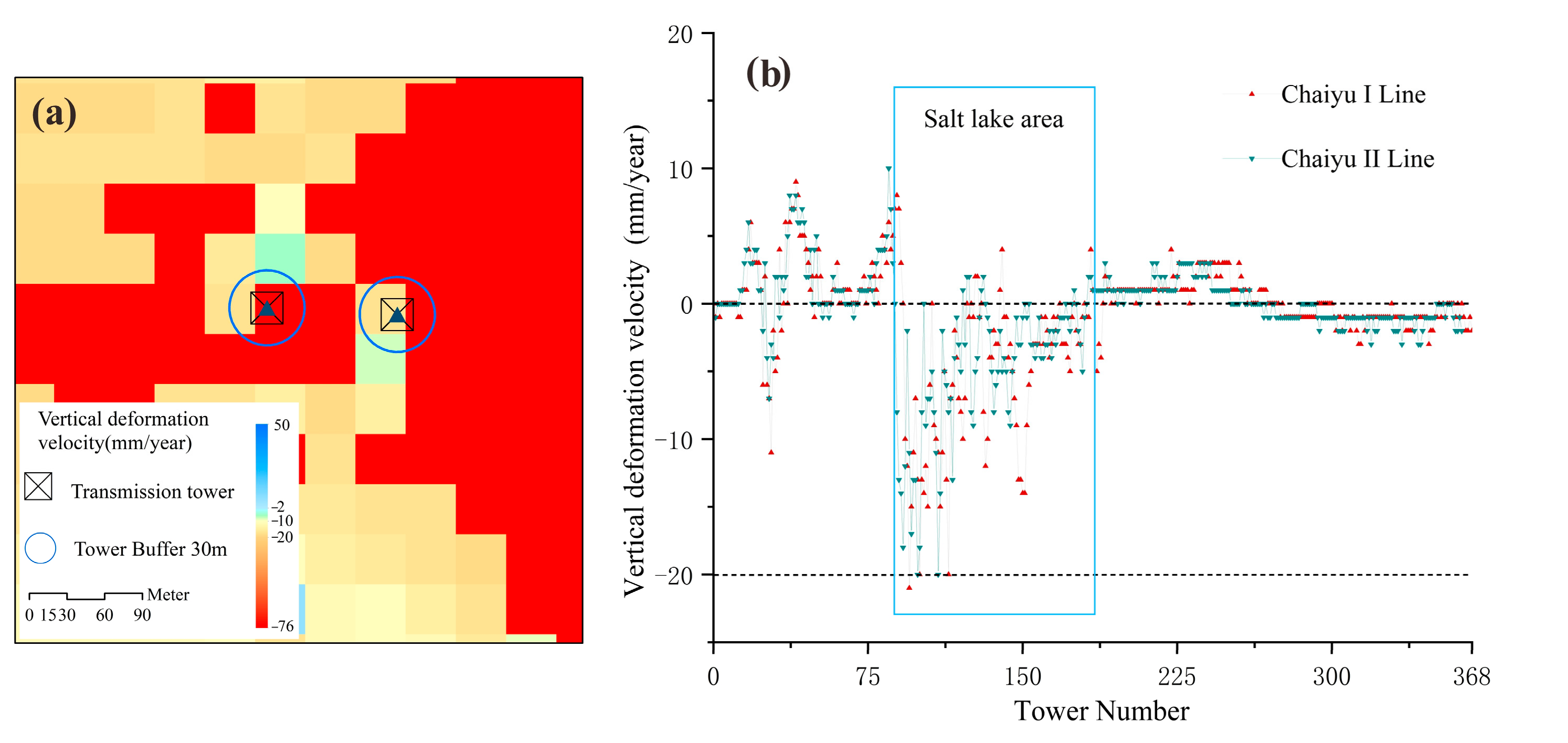
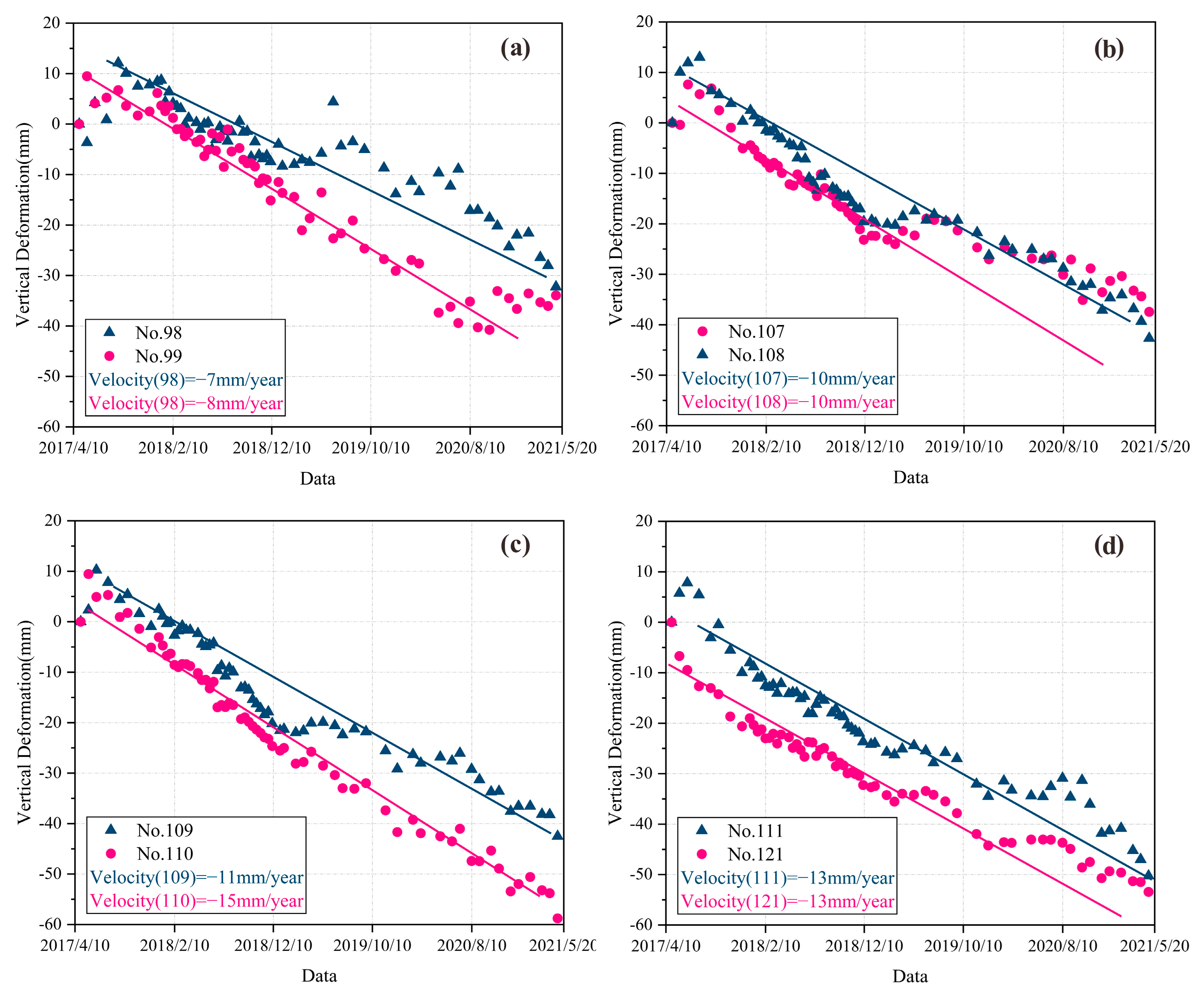
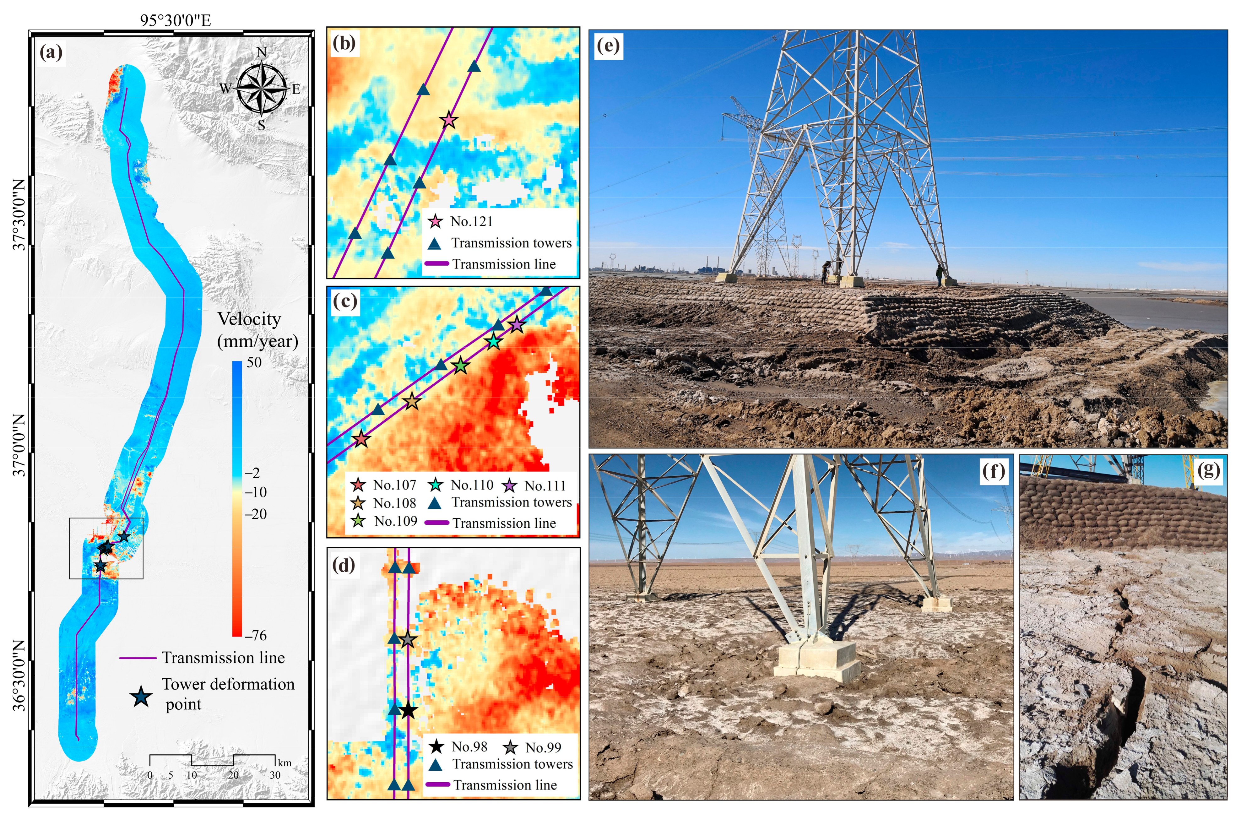
3.2. Deformation of Transmission Lines and Typical Towers

The foundation size of the transmission tower in the study area is about 15 × 15 m. During the data processing, the raster cell was converted to 40 × 40 m. To reduce the transmission tower displacement error caused by a single raster cell, we buffered the tower center by 30 m, as shown in Figure 6a. Then, we averaged the values within the range to obtain the transmission tower vertical deformation velocity and the line deformation, as shown in Figure 6b. According to the land subsidence along the line, the transmission towers’ most serious land subsidence area is mainly in the central Salt Lake area, which is consistent with the field deformation.

In order to further analyze the time-series deformation of the tower, No. 98, 99, 107, 108, 109, 110, 111, 121 was selected. The deformation results were described in

Table 3. Typical tower vertical deformation results.

Tower Number	Cumulative Vertical Deformation (mm)	Average Vertical Deformation Velocity (mm/Year)	Location
98	−29	−7	Figure 7a
99	−34	−8	Figure 7a
107	−41	−10	Figure 7b
108	−37	−10	Figure 7b
109	−44	−11	Figure 7c
110	−60	−15	Figure 7c
111	−50	−13	Figure 7d
121	−55	−13	Figure 7d

.

From Figure 7a–d, it can be seen that most of the ground vertical deformation maps of transmission towers are linear. This may be related to the continuous exploitation of underground brine in the area. Some transmission towers show certain volatility in vertical displacement, which may be associated with the expansion of mineral salt, precipitation, and human disturbance.

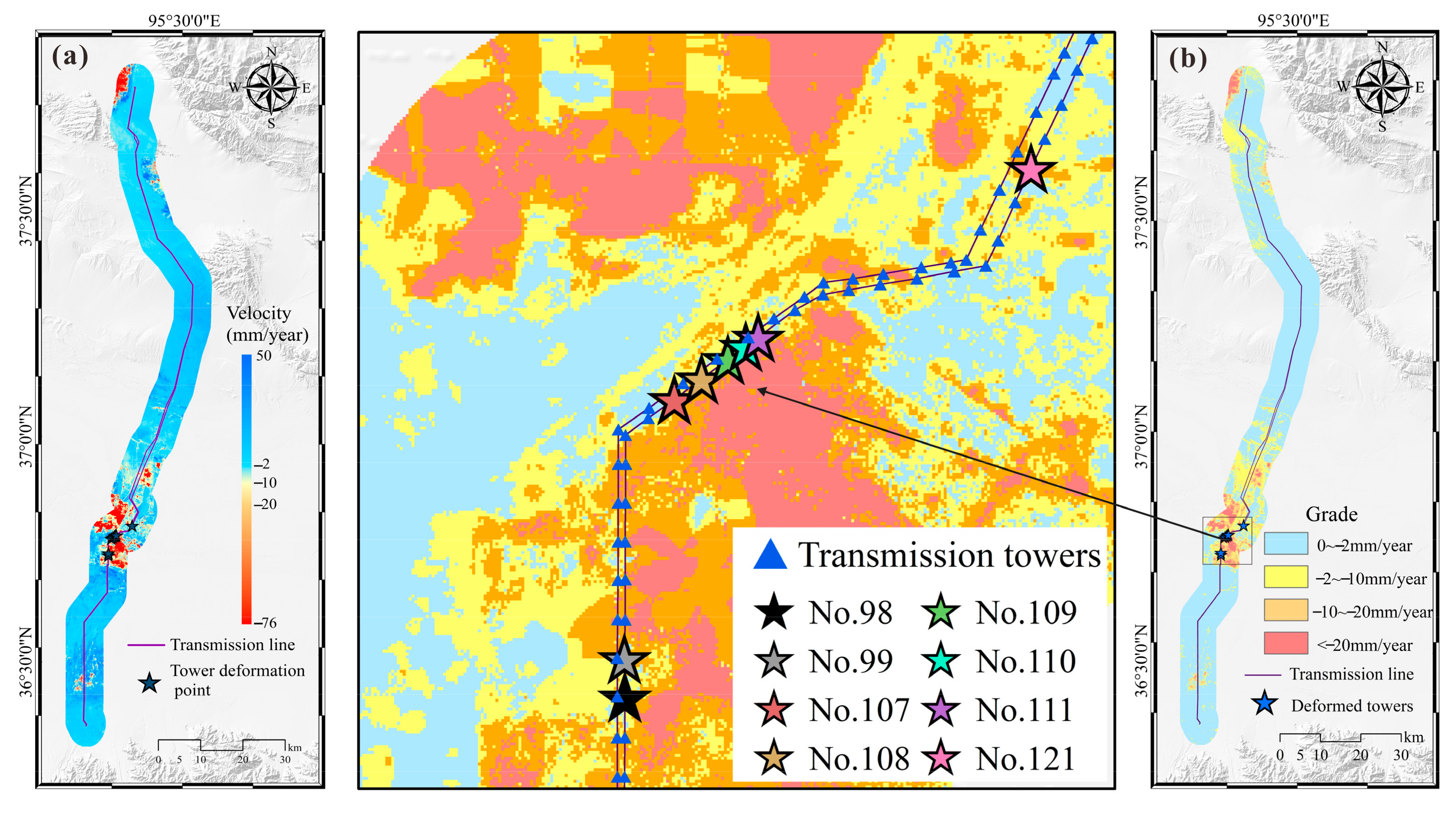
3.3. K-Means Land Subsidence Intensity Classification

Since the UHV transmission line is distributed in the central and northern parts of the Salt Lake area, during the local industrial production of mineral salt activities, irregular exploitation of underground brine for drying causes significant changes in surface water. This causes the persistent scatterer density of SAR data to be relatively low. Therefore, to overcome this limitation and to study the land subsidence along the UHV transmission line more comprehensively, we used the Kriging interpolation in GIS tools to construct the persistent scatterer density point interpolation. The land subsidence information of the whole study area is shown in Figure 8a.

In this study, according to the land subsidence along the transmission line and the field investigation results, the towers with positive deformation velocity points were not considered and removed. The remaining towers were clustered, and three clustering centers were obtained: −1.98, −10.13, and −18.09. Combined with the relevant specifications of electric power [37,38,39], the land subsidence intensities are divided into four grades, as shown in Figure 8b.

3.4. FR

In

Table 4. Relationship between different land subsidence intensities and conditioning factors using frequency ratio (FR) model.

Conditioning Factor	Class/ Category	Ratio Each Class	Grade of −2~−10 mm/Year Ratio of Occurrence	Grade of −10~−20 mm/Year Ratio of Occurrence	Grade of <−20 mm/Year Ratio of Occurrence	Grade of−2~−10 mm/Year FR	Grade of−10~−20 mm/Year FR	Grade of<−20 mm/Year FR
Slope (degree)	0~5	0.7774	0.6881	0.8438	0.8716	0.8852	1.0854	1.1212
	5~20	0.1979	0.2396	0.1425	0.1133	1.2109	0.7203	0.5727
	>20	0.0247	0.0722	0.0134	0.0151	2.9217	0.5543	0.6098
Profile curvature	−0.2	0.0770	0.1050	0.0836	0.0825	1.3647	1.0871	1.0725
	−0.2~0	0.5006	0.4615	0.5184	0.5325	0.9219	1.0356	1.0637
	0~0.2	0.3461	0.3293	0.3282	0.3259	0.9513	0.9483	0.9414
	>0.2	0.0763	0.1042	0.0697	0.0591	0.3655	0.9129	0.7746
Plan curvature	<−1	0.0694	0.0901	0.0716	0.0714	1.2992	1.0312	1.0283
	−1~0.01	0.5646	0.5215	0.5960	0.6054	0.9237	1.0554	1.0722
	0.01~0.02	0.2944	0.2870	0.2721	0.2653	0.9746	0.9240	0.9011
	>0.02	0.0716	0.1013	0.0604	0.0580	1.4160	0.8450	0.8097
Lithology map	Chemical deposits	0.2442	0.5428	0.6927	0.5234	2.2225	2.8363	2.1433
	Marsh sediment	0.0864	0.0191	0.0304	0.0437	0.2211	0.3521	0.5059
	Lake sediments	0.0336	0.0386	0.1600	0.3108	1.1479	4.7637	9.2528
	Flood deposits	0.2242	0.0635	0.0734	0.1108	0.2834	0.3276	0.4944
	Alluvial deposits	0.1218	0.1108	0.0386	0.0102	0.9098	0.3169	0.8369
	aeolian deposits	0.0469	0.0110	0.0048	0.0010	0.2352	0.1028	0.0214
	Extremely hard rock	0.1927	0.0783	0	0	0.4060	0	0
	hard rock	0.0501	0.1359	0	0	2.7146	0	0
Distance to river map (m)	0~300	0.0430	0.0389	0.0895	0.0841	0.9054	2.0806	1.9561
	300~600	0.0407	0.0289	0.0780	0.0818	0.7009	1.9181	2.0122
	600~900	0.0702	0.0424	0.1065	0.1275	0.6048	1.5170	1.8171
	>900	0.8641	0.8897	0.7260	0.7065	1.0515	0.8581	0.8350
TWI	<6	0.1687	0.2157	0.0930	0.0694	1.2788	0.5507	0.4112
	6~13	0.4323	0.3843	0.3974	0.4016	0.8890	0.9194	0.9290
	13~25	0.1364	0.1187	0.1381	0.1454	0.8703	1.0119	1.0660
	>25	0.2626	0.2813	0.3716	0.3836	1.0711	1.4151	1.4608
Distance to road map (m)	0~400	0.1547	0.6080	0.2163	0.1606	3.9294	1.3980	1.0380
	400~800	0.1295	0.1715	0.1437	0.1771	1.3240	1.1095	1.3671
	800~1200	0.1157	0.1116	0.1265	0.1241	0.9646	1.0932	1.0727
	>1200	0.6003	0.1090	0.5135	0.5382	0.1814	0.8554	0.8966
Land-use map	Residential	0.0288	0.0248	0.0272	0.0288	0.8602	0.9465	0.9995
	Vegetation	0.1115	0.0852	0.1816	0.2465	0.7641	1.6286	2.2099
	Water	0.0049	0.0084	0.0026	0	1.7254	0.5241	0
	Bare	0.7760	0.7336	0.2509	0.1191	0.9455	0.3234	0.1535
	Saltern	0.0789	0.1480	0.5376	0.6056	1.8765	6.8183	7.6803

, we mark FR values >1 in bold. At the slope grade >20°, the maximum FR value of −2~−10 mm/year is 2.9217. This may relate to the mountain deformation caused by freeze–thaw erosion, rain erosion, wind erosion, etc. The FR value of three intensities is greater than 2 in the chemical sediments category, indicating that the area is closely related to land subsidence. In the lake sediments category, the FR value at the <−20 mm/year grade reaches the maximum of 9.2528, indicating that the area is prone to large ground deformation. In the class of land-use map, the FR values of land subsidence in the saltern area are more considerable, and the maximum value at the <−20 mm/year grade is 7.6803, indicating that mining mineral salt in this area may produce large land subsidence.

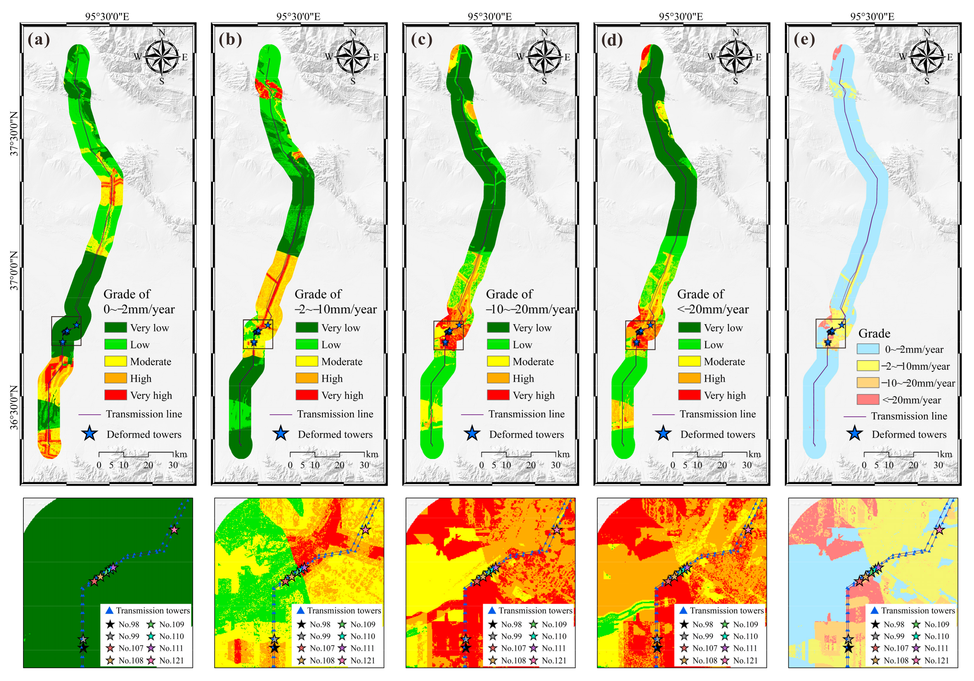
3.5. Land Subsidence Susceptibility Map

To evaluate the susceptibility of different land subsidence intensities along the UHV transmission line, we used the different land subsidence intensities as the data source, which were divided by the K-means method. Then, the susceptibility map of different land subsidence intensities through the MLPNN was produced using the selected eight land subsidence conditioning factors. The susceptibility map of different land subsidence intensities is divided into extremely low, low, medium, high, and very high susceptibility by using the quantile classification method [51,61].

On the susceptibility map, among the four grades of different land subsidence intensities, the areas of high and very high susceptibility (marked orange and red, respectively, in Figure 9c,d) were most frequently found near the central Salt Lake area and were partially distributed on both sides of the road (Figure 9a,b). High and very high susceptibility (marked orange and red, respectively, in Figure 9c,d) at the −10~−20 and <−20 mm/year grades were mainly near Salt Lakes’ rivers. This may be related to the exploitation of mineral salts and river erosion. High and very high susceptibility (marked orange and red, respectively, in Figure 9b) of −2~−10 mm/year mainly occurred on the central Salt Lake highway and the lithology of extremely hard rock in the north. The high and very high susceptibility in the central area may be related to the subsidence deformation of saline soil caused by dynamic vehicle load. However, in northern mountainous areas, it may be caused by freeze–thaw erosion, rain erosion, wind erosion, etc. High and very high susceptibility (marked orange and red, respectively, in Figure 9a) of 0~−2 mm/year were mainly distributed on both sides of the road. This may be related to vehicles’ dynamic loads.

To obtain the susceptibility distribution map of different land subsidence intensities in the whole area, we compared the four intensities calculation results in the same raster. The intensity of the maximum value was taken as the attribute of the raster, as shown in

Table 5. The example of susceptibility comparison of raster land subsidence grade.

Raster FID	Grade of 0~−2 mm/Year	Grade of −2~−10 mm/Year	Grade of −10~−20 mm/Year	Grade of <−20 mm/Year	The Maxmium Susceptibility Value
1	0.998	0.137	0.282	0.514	Grade of 0~−2 mm/year
10623	0.635	0.876	0.752	0.631	Grade of −2~−10 mm/year
146269	0.463	0.568	0.625	0.534	Grade of −10~−20 mm/year
501516	0.528	0.324	0.685	1	Grade of <−20 mm/year
…	…	…	…	…	…

. Finally, the distribution of all land subsidence intensities was obtained, as shown in Figure 9e. It can be observed from Figure 9e that most of the towers in the Salt Lake area are located in an area of severe land subsidence intensity. The maximum land subsidence intensity of the deformed tower is at the <−20 mm/year grade.

3.6. Model Validation

The ROC curve has been used to evaluate the accuracy of the MLPNN in different land subsidence intensities [70,71]. An ROC curve analysis is a standard method to verify probability models used to generate land subsidence susceptibility maps according to the area under the curve (AUC) [49,50]. Higher values of the AUC under the ROC curve indicate more accurate and reliable models.

The susceptibility map of land subsidence intensities generated by MLPNN under different land subsidence intensities was used for comparative analysis. The ROC curves of four different land subsidence intensities are shown in Figure 10. The largest AUC of 0.951 was at the <−20 mm/year grade (red line in Figure 10), followed by 0.926 at the −10~−20 mm/year grade (green line in Figure 10), 0.879 at the 0~−2 mm/year grade (blue line in Figure 10), and 0.812 at the −2~−10 mm/year grade (yellow line in Figure 10).

If the AUC is lower than 0.5, the model is considered to be unacceptably inaccurate [70]. Since the AUC values of the evaluation results in this study are all greater than 0.5, the generated susceptibility map of land subsidence can be used to predict the high-susceptibility areas of land subsidence intensity along the UHV transmission line.

4. Discussion

4.1. Land Subsidence Map of SBAS-InSAR

Based on the Sentinel-1 datasets collected from April 2017 to May 2021, the deformation time-series map of the area was generated using the SBAS-InSAR method to analyze the ground subsidence along the UHV transmission line. Then, the vertical deformation map was obtained by transforming the deformation time-series maps [8,51].

The results indicate that the land subsidence located in the study area is mainly concentrated in the Salt Lake area in the middle of the transmission line. This is consistent with the actual deformation of the transmission tower (Figure 5a–d) [2]. From the perspective of the whole study area, the land subsidence in the central Salt Lake area shows a spatial distribution trend of the central funnel. As one of the largest mineral salt production bases in China, the large number of underground brine mines in the Salt Lake area may affect dynamic changes in the underground aquifer system, thereby affecting the stability of the overlying soil layer [72]. Most of the UHV transmission line runs parallel along the main traffic lines, such as the Qinghai–Tibet Railway and highway (Figure 1). Frequently vehicle loads may change soil structure stability and cause foundation instability [12].

By analyzing the 4-year vertical deformation time-series maps along the UHV transmission line (Figure 7a–d), it can be predicted that transmission towers crossing the central Salt Lake area still have the probability of deformation and failure in the future [33]. Increased salt production in this area will lead to excessive exploitation of underground brine and affect the speed of land subsidence [33,73]. To better study the deformation of transmission towers in this area, it is necessary to analyze the data analysis based on groundwater level and further solve the details between groundwater change and transmission tower deformation. Therefore, in future research, airborne electromagnetic data could be integrated with subsidence data by InSAR to effectively simulate the complex space-time process of surface deformation [74]. At the same time, future research should focus on intelligent picture recognition of tower deformation [75].

However, due to the long span of the UHV transmission line, only one scene of Sentinel-1 data cannot be covered entirely. Therefore, it takes time and manpower to interpret the land subsidence inventory maps. In this study, for comparing and analyzing the existing processing methods, the SABAS-InSAR method was selected as a suitable method for the study area [33,51,52]. Regarding datasets processing, a vast amount of data still has some shortcomings in the interpretation results, and several optimization methods have been proposed [22,76,77,78,79,80,81]. This will be an essential reference for future research on transmission towers to improve efficiency and obtain more accurate interpretation results.

4.2. Land Subsidence Intensity Classification

Unlike previous land subsidence susceptibility evaluation studies [8,51,52], the main focus of this study is the susceptibility evaluation of different land subsidence intensities along a UHV transmission line. We obtained the vertical deformation map of ground subsidence along the UHV transmission line by using the SBAS-InSAR method and considered both the size of the raster and the transmission tower in the study area. The vertical deformation of the raster at the coordinate point of the transmission tower is not equal to that of the whole transmission tower [13,39]. The land subsidence value of the tower area was obtained by buffering the transmission tower coordinate points and averaging the vertical deformation value of the raster in the buffer area. However, to obtain the average land subsidence velocity of the location of the transmission tower, in this study, we selected a more appropriate raster size and without considering the towers that deformation velocity is positive. Considering that no more suitable research methods have been found and transmission towers lack ground GPS monitoring results, we used the above classification as subsequent land subsidence susceptibility map sample datasets.

After receiving the vertical deformation of the entire UHV transmission line, the K-means method was used to classify the vertical deformation velocity [60] and to obtain the results for the four land subsidence intensity grades. Then, we deleted the points where the towers’ vertical deformations were greater than 0 according to the vertical deformation of the whole transmission line and classified the deformation results of the remaining parts by the K-means method. Through the classification results, it can be found that the deformation and damage of the investigated towers are mainly concentrated at two grades, i.e., −10~−20 mm/year and <−20 mm/year, which has important guiding significance for future treatment and protection of towers.

4.3. Land Subsidence Susceptibility Map

Accurate land subsidence susceptibility maps of different land subsidence intensities are important for future planning, design, protection and operations management of UHV transmission lines. In this study, we used the SBAS-InSAR method to obtain the land subsidence inventory map along the UHV transmission line. Combined with the classification of different land subsidence intensities, the MLPNN model was used to obtain the susceptibility map of different land subsidence intensities [8,51]. Unfortunately, during the process of collecting land subsidence susceptibility conditioning factors in the study area, the distribution of groundwater in the study area was not collected due to limited conditions [33,52]. However, from the spatial location of land subsidence distribution, the saltern area located in the lowest depression of the study area is the most concentrated area of land subsidence (Figure 5a, Figure 9b–e).

This compensates, to some extent, for the error caused by the lack of groundwater distribution data. Although the UHV transmission line has a long span between the north and south, the average annual precipitation is scarce due to the dry and hot climate in the northwest inland of China [33,82], and therefore, the influence of precipitation distribution on the susceptibility of different land subsidence intensities was not considered in this study [72].

The ROC curve was used to evaluate the accuracy of the susceptibility mapping of different land subsidence intensities along the UHV transmission line (Figure 10). The AUC value showed that the highest prediction accuracy of susceptibility classification was 0.951 at the <−20 mm/year grade, followed by 0.926 at the −10~−20 mm/year grade, 0.879 at the 0~−2 mm/year grade, and 0.812 at the −2~−10 mm/year grade. The susceptibility map of different land subsidence intensities shows that transmission towers are mostly located in the high and very high susceptibility ranges at the <−20 mm/year grade and the −10~20 mm/year grade. This result can more accurately and quickly identify the disaster of transmission tower settlement. It can be used as the basis for preventing and controlling the deformation and failure of transmission towers of the State Grid in the Salt Lake area in the future. At the same time, the method adopted in this study of combining InSAR datasets with the susceptibility of different land subsidence intensities can provide new ideas for other areas.

5. Conclusions

In this study, we used the SBAS-InSAR method to generate the land subsidence inventory map along a UHV transmission line. The results show that the land subsidence is mainly concentrated in the central Salt Lake area (Figure 5), and the maximum land subsidence velocity of the transmission tower is 15 mm/year (Figure 7). After obtaining the deformation results of the UHV transmission line, the K-means method was used to classify the deformation intensity. Eight potential factors related to subsidence were analyzed to identify the conditioning factors of land subsidence, and the frequency ratio model was used to obtain the relationships among different land subsidence intensities and various conditioning factors. The MLPNN was used for susceptibility evaluation, and the accuracy was tested using the ROC curve. The susceptibility map of different land subsidence intensities shows that Salt Lake’s central part is a high and extremely high-susceptibility area. The human activities of underground brine extraction and mineral salt production in this area may affect the subsidence of this area. The AUC values of the land subsidence intensity grades were calculated by the ROC analysis. The AUC value indicated that the prediction results of each land subsidence intensity grade were excellent. Among them, the AUC value at the <−20 mm/year grade was the highest, which was 0.951, then 0.926 at the −10~−20 mm/year grade, 0.879 at the 0~−2 mm/year grade, and 0.812 at the −2~−10 mm/year grade. This shows that the susceptibility map we generated of different land subsidence intensities along the UHV transmission line is valuable. At the same time, the susceptibility classification results of different land subsidence intensities are consistent with the interpretation and site tower deformation. Although the datasets used in this study are limited, since the AUC values of the evaluation results in this study are all greater than 0.5, the results are accurate and reliable. The generated susceptibility map of land subsidence intensities can be used to predict the high-susceptibility areas of different land subsidence intensities along UHV transmission lines, which is important to the planning, design, protection, and operations management of transmission line towers.

References

1. Yu, Q.; Ji, Y.; Zhang, Z.; Wen, Z.; Feng, C. Design and research of high voltage transmission lines on the Qinghai-Tibet Plateau-A Special Issue on the Permafrost Power Lines. Cold Reg. Sci. Technol. 2016, 121, 179–186. [Google Scholar] [CrossRef]
2. Qi, Z.X.; Wang, X.J.; Liu, C.Q. Analysis on Collapsible Deformation and Prevention Measures of Transmission Line Tower Ground in Qarhan Salt Lake Area. Electr. Power Surv. Des. 2021, 5, 72–76. [Google Scholar]
3. Tan, Q.; Man, Y.; Gao, W.; Tong, W.; Zheng, W. Research on design selection analysis and anti-Corrosion treatment of the transmission line tower foundation in Salt Lake area. Power Syst. Clean Energy 2012, 28, 51–56. [Google Scholar]
4. Zheng, W.; Man, Y.; Yu, X.; Tan, Q.; Tong, W.; Gong, X.; Liu, Y.; Zhang, J.; Zhu, A. Research on settlement control of the transmission line foundation in Salt Lake area. Power Syst. Clean Energy 2013, 29, 16–19. [Google Scholar]
5. Lixin, Y.; Fang, Z.; He, X.; Shijie, C.; Wei, W.; Qiang, Y. Land subsidence in Tianjin, China. Environ. Earth Sci. 2011, 62, 1151–1161. [Google Scholar] [CrossRef]
6. Jiang, C. Monitoring and Analysis of Ground Subsidence of East China. In Proceedings of the 2015 International Conference on Management, Education, Information and Control, Shenyang, China, 29–31 May 2015. [Google Scholar]
7. Xue, Y.; Zhang, Y.; Ye, S.; Wu, J.; Li, Q. Land subsidence in China. Environ. Geol. 2005, 48, 713–720. [Google Scholar] [CrossRef]
8. Fadhillah, M.F.; Achmad, A.R.; Lee, C. Integration of InSAR Time-Series Data and GIS to Assess Land Subsidence along Subway Lines in the Seoul Metropolitan Area, South Korea. Remote Sens. 2020, 12, 3505. [Google Scholar] [CrossRef]
9. Galloway, D.L.; Burbey, T.J. Review: Regional land subsidence accompanying groundwater extraction. Hydrogeol. J. 2011, 19, 1459–1486. [Google Scholar] [CrossRef]
10. Holzer, T.L.; Galloway, D.L.; Ehlen, J.; Haneberg, W.C.; Larson, R.A. Impacts of land subsidence caused by withdrawal of underground fluids in the United States. In Reviews in Engineering Geology XVI: Humans as Geologic Agents; Geological Society of America: Boulder, CO, USA, 2005; pp. 87–99. [Google Scholar] [CrossRef] [Green Version]
11. Lixin, Y.; Jie, W.; Chuanqing, S.; Guo, J.; Yanxiang, J.; Liu, B. Land Subsidence Disaster Survey and Its Economic Loss Assessment in Tianjin, China. Nat. Hazards Rev. 2010, 11, 35–41. [Google Scholar] [CrossRef]
12. Liu, J.Y.; Liu, J.H.; Ding, B. Analysis of Subsidence Monitoring of the Saline Soft Soil Ground in Qarham Salt Lake District. Adv. Mater. Res. 2012, 503–504, 1247–1255. [Google Scholar] [CrossRef]
13. Wei, Z.Y. Harm of Qinghai Saline Soil to Power Transformation Engineering and Treatment Measure. Qinghai Electr. Power 2007, S1, 40–44. [Google Scholar]
14. Fergason, K.C.; Rucker, M.L.; Panda, B.B. Methods for monitoring land subsidence and earth fissures in the Western USA. Proc. Int. Assoc. Hydrol. Sci. 2015, 372, 361–366. [Google Scholar] [CrossRef]
15. Abidin, H.Z.; Djaja, R.; Darmawan, D.; Hadi, S.; Akbar, A.; Rajiyowiryono, H.; Sudibyo, Y.; Meilano, I.; Kasuma, M.A.; Kahar, J.; et al. Land Subsidence of Jakarta (Indonesia) and its Geodetic Monitoring System. Nat. Hazards 2001, 23, 365–387. [Google Scholar] [CrossRef]
16. Wang, J.; Wang, C.; Zhang, H.; Tang, Y.; Duan, W.; Dong, L. Freeze-Thaw Deformation Cycles and Temporal-Spatial Distribution of Permafrost along the Qinghai-Tibet Railway Using Multitrack InSAR Processing. Remote Sens.-Basel. 2021, 13, 4744. [Google Scholar] [CrossRef]
17. Guo, L.; Xie, Y.; Yu, Q.; You, Y.; Wang, X.; Li, X. Displacements of tower foundations in permafrost regions along the Qinghai-Tibet Power Transmission Line. Cold Reg. Sci. Technol. 2016, 121, 187–195. [Google Scholar] [CrossRef]
18. Zhang, Z.; Wang, M.; Liu, X.; Wang, C.; Zhang, H.; Tang, Y.; Zhang, B. Deformation feature analysis of Qinghai-Tibet railway using terraSAR-X and sentinel-1A time-series interferometry. IEEE J. Sel. Top. Appl. Earth Obs. Remote Sens. 2019, 12, 5199–5212. [Google Scholar] [CrossRef]
19. Ferretti, A.; Prati, C.; Rocca, F. Permanent scatterers in SAR interferometry. IEEE Trans. Geosci. Remote Sens. 2001, 39, 8–20. [Google Scholar] [CrossRef]
20. Fobert, M.; Singhroy, V.; Spray, J.G. InSAR Monitoring of Landslide Activity in Dominica. Remote Sens. 2021, 13, 815. [Google Scholar] [CrossRef]
21. Zhang, L.; Dai, K.; Deng, J.; Ge, D.; Liang, R.; Li, W.; Xu, Q. Identifying Potential Landslides by Stacking-InSAR in Southwestern China and Its Performance Comparison with SBAS-InSAR. Remote Sens. 2021, 13, 3662. [Google Scholar] [CrossRef]
22. Zhou, C.; Cao, Y.; Yin, K.; Wang, Y.; Shi, X.; Catani, F.; Ahmed, B. Landslide Characterization Applying Sentinel-1 Images and InSAR Technique: The Muyubao Landslide in the Three Gorges Reservoir Area, China. Remote Sens. 2020, 12, 3385. [Google Scholar] [CrossRef]
23. Li, X.; Yan, L.; Lu, L.; Huang, G.; Zhao, Z.; Lu, Z. Adjacent-Track InSAR Processing for Large-Scale Land Subsidence Monitoring in the Hebei Plain. Remote Sens. 2021, 13, 795. [Google Scholar] [CrossRef]
24. Zhou, C.; Gong, H.; Chen, B.; Li, J.; Gao, M.; Zhu, F.; Chen, W.; Liang, Y. InSAR Time-Series Analysis of Land Subsidence under Different Land Use Types in the Eastern Beijing Plain, China. Remote Sens. 2017, 9, 380. [Google Scholar] [CrossRef] [Green Version]
25. Han, Y.; Zou, J.; Lu, Z.; Qu, F.; Kang, Y.; Li, J. Ground Deformation of Wuhan, China, Revealed by Multi-Temporal InSAR Analysis. Remote Sens. 2020, 12, 3788. [Google Scholar] [CrossRef]
26. Hu, B.; Wang, H.; Sun, Y.; Hou, J.; Liang, J. Long-Term Land Subsidence Monitoring of Beijing (China) Using the Small Baseline Subset (SBAS) Technique. Remote Sens. 2014, 6, 3648–3661. [Google Scholar] [CrossRef] [Green Version]
27. Zhou, L.; Guo, J.; Hu, J.; Li, J.; Xu, Y.; Pan, Y.; Shi, M. Wuhan Surface Subsidence Analysis in 2015-2016 Based on Sentinel-1A Data by SBAS-InSAR. Remote Sens. 2017, 9, 982. [Google Scholar] [CrossRef] [Green Version]
28. Wang, D.; Liu, J.; Li, X. Numerical Simulation of Coupled Water and Salt Transfer in Soil and a Case Study of the Expansion of Subgrade composed by Saline Soil. Procedia Eng. 2016, 143, 315–322. [Google Scholar] [CrossRef] [Green Version]
29. Lai, Y.; Wu, D.; Zhang, M. Crystallization deformation of a saline soil during freezing and thawing processes. Appl. Therm. Eng. 2017, 120, 463–473. [Google Scholar] [CrossRef]
30. Wang, W.; Wu, L.; Gong, H.; Fan, P.; Wu, W.; Zhou, Y.; Zhang, Z. Deformation Monitoring for High-Voltage Transmission Lines Using Sentinel-1A Data. IOP Conf. Ser. Earth Environ. Sci. 2019, 252, 32033. [Google Scholar] [CrossRef] [Green Version]
31. He, H.; Zhou, L.; Lee, H. Ground Displacement Variation Around Power Line Corridors on the Loess Plateau Estimated by Persistent Scatterer Interferometry. IEEE Access. 2021, 9, 87908–87917. [Google Scholar] [CrossRef]
32. Higgins, S.A. Review: Advances in delta-subsidence research using satellite methods. Hydrogeol. J. 2016, 24, 587–600. [Google Scholar] [CrossRef]
33. Xiang, W.; Zhang, R.; Liu, G.; Wang, X.; Mao, W.; Zhang, B.; Cai, J.; Bao, J.; Fu, Y. Extraction and analysis of saline soil deformation in the Qarhan Salt Lake region (in Qinghai, China) by the sentinel SBAS-InSAR technique. Geod. Geodyn. 2021, 13, 127–137. [Google Scholar] [CrossRef]
34. Hu, B.; Zhou, J.; Wang, J.; Chen, Z.; Wang, D.; Xu, S. Risk assessment of land subsidence at Tianjin coastal area in China. Environ. Earth Sci. 2009, 59, 269–276. [Google Scholar] [CrossRef]
35. Guo, Z.; Chen, L.; Yin, K.; Shrestha, D.P.; Zhang, L. Quantitative risk assessment of slow-moving landslides from the viewpoint of decision-making: A case study of the Three Gorges Reservoir in China. Eng. Geol. 2020, 273, 105667. [Google Scholar] [CrossRef]
36. Wang, H.; Wang, Y.; Jiao, X.; Qian, G. Risk management of land subsidence in Shanghai. Desalin. Water Treat. 2014, 52, 1122–1129. [Google Scholar] [CrossRef]
37. China Federation of Electric Power Enterprises. Code for Design of 110 kv~750 kv Overhead Transmission Line; People’s Publishing House: Beijing, China, 2010. [Google Scholar]
38. State Grid Corporation; Northeast Electric Power Design Institute. Design Manual of Power Engineering High Voltage Transmission Lines; China Electric Power Publishing House: Beijing, China, 2003. [Google Scholar]
39. Shi, Z. Settlement and treatment scheme of linear self-supporting tower foundation of transmission line in goaf. Shanxi Electr. Power Technol. 1997, 3, 19–21. [Google Scholar]
40. Taravatrooy, N.; Nikoo, M.R.; Sadegh, M.; Parvinnia, M. A hybrid clustering-fusion methodology for land subsidence estimation. Nat. Hazards 2018, 94, 905–926. [Google Scholar] [CrossRef] [Green Version]
41. Zhang, Y.; Du, L.; Liu, J. Identifying the reuse patterns of coal mining subsidence areas: A case-study of Jixi City (China). Land Degrad. Dev. 2021, 32, 4858–4870. [Google Scholar] [CrossRef]
42. Sarmin, F.J.; Zaman, M.S.U.; Sarkar, A.R. Monitoring land deformation due to groundwater extraction using Sentinel-1 satellite images: A case study from Chapai Nawabgonj, Bangladesh. In Proceedings of the 2020 23rd International Conference on Computer and Information Technology, Dhaka, Bangladesh, 19–21 December 2020; pp. 1–6. [Google Scholar]
43. Rahmati, O.; Falah, F.; Naghibi, S.A.; Biggs, T.; Soltani, M.; Deo, R.C.; Cerdà, A.; Mohammadi, F.; Tien Bui, D. Land subsidence modelling using tree-based machine learning algorithms. Sci. Total Environ. 2019, 672, 239–252. [Google Scholar] [CrossRef]
44. Tien Bui, D.; Shahabi, H.; Shirzadi, A.; Chapi, K.; Pradhan, B.; Chen, W.; Khosravi, K.; Panahi, M.; Bin Ahmad, B.; Saro, L. Land Subsidence Susceptibility Mapping in South Korea Using Machine Learning Algorithms. Sensors 2018, 18, 2464. [Google Scholar] [CrossRef] [Green Version]
45. Arabameri, A.; Saha, S.; Roy, J.; Tiefenbacher, J.P.; Cerda, A.; Biggs, T.; Pradhan, B.; Thi, N.P.; Collins, A.L. A novel ensemble computational intelligence approach for the spatial prediction of land subsidence susceptibility. Sci. Total Environ. 2020, 726, 138595. [Google Scholar] [CrossRef]
46. Elmahdy, S.I.; Mohamed, M.M.; Ali, T.A.; Abdalla, J.E.; Abouleish, M. Land subsidence and sinkholes susceptibility mapping and analysis using random forest and frequency ratio models in Al Ain, UAE. Geocarto Int. 2022, 37, 315–331. [Google Scholar] [CrossRef]
47. Lee, S.; Park, I.; Choi, J. Spatial Prediction of Ground Subsidence Susceptibility Using an Artificial Neural Network. Environ. Manag. 2012, 49, 347–358. [Google Scholar] [CrossRef] [PubMed]
48. Pradhan, B. A comparative study on the predictive ability of the decision tree, support vector machine and neuro-fuzzy models in landslide susceptibility mapping using GIS. Comput. Geosci. 2013, 51, 350–365. [Google Scholar] [CrossRef]
49. Mohammady, M.; Pourghasemi, H.R.; Amiri, M. Land subsidence susceptibility assessment using random forest machine learning algorithm. Environ. Earth Sci. 2019, 78, 1–12. [Google Scholar] [CrossRef]
50. Abdollahi, S.; Pourghasemi, H.R.; Ghanbarian, G.A.; Safaeian, R. Prioritization of effective factors in the occurrence of land subsidence and its susceptibility mapping using an SVM model and their different kernel functions. Bull. Eng. Geol. Environ. 2019, 78, 4017–4034. [Google Scholar] [CrossRef]
51. Hakim, W.; Achmad, A.; Lee, C. Land Subsidence Susceptibility Mapping in Jakarta Using Functional and Meta-Ensemble Machine Learning Algorithm Based on Time-Series InSAR Data. Remote Sens. 2020, 12, 3627. [Google Scholar] [CrossRef]
52. Ranjgar, B.; Razavi-Termeh, S.V.; Foroughnia, F.; Sadeghi-Niaraki, A.; Perissin, D. Land Subsidence Susceptibility Mapping Using Persistent Scatterer SAR Interferometry Technique and Optimized Hybrid Machine Learning Algorithms. Remote Sens. 2021, 13, 1326. [Google Scholar] [CrossRef]
53. Jin, B.; Yin, K.; Gui, L.; Zhao, B.; Guo, B.; Zeng, T. Based on remote sensing interpretation of transmission line tower land subsidence susceptibility evaluation in Salt Lake area. Earth Sci. 2022, accepted. [Google Scholar]
54. Li, G.; Tan, Q.; Xie, C.; Fei, X.; Ma, X.; Zhao, B.; Ou, W.; Yang, Z.; Wang, J.; Fang, H. The Transmission Channel Tower Identification and Landslide Disaster Monitoring Based on InSAR. Int. Arch. Photogramm. Remote Sens. Spat. Inf. Sci. 2018, XLII-3, 807–813. [Google Scholar] [CrossRef] [Green Version]
55. Yunjun, Z.; Fattahi, H.; Amelung, F. Small baseline InSAR time series analysis: Unwrapping error correction and noise reduction. Comput. Geosci. 2019, 133, 104331. [Google Scholar] [CrossRef] [Green Version]
56. Floris, M.; Fontana, A.; Tessari, G.; Mulè, M. Subsidence Zonation Through Satellite Interferometry in Coastal Plain Environments of NE Italy: A Possible Tool for Geological and Geomorphological Mapping in Urban Areas. Remote Sens. 2019, 11, 165. [Google Scholar] [CrossRef] [Green Version]
57. Pepe, A.; Bonano, M.; Zhao, Q.; Yang, T.; Wang, H. The Use of C-/X-Band Time-Gapped SAR Data and Geotechnical Models for the Study of Shanghai’s Ocean-Reclaimed Lands through the SBAS-DInSAR Technique. Remote Sens. 2016, 8, 911. [Google Scholar] [CrossRef] [Green Version]
58. Ren, H.; Feng, X. Calculating vertical deformation using a single InSAR pair based on singular value decomposition in mining areas. Int. J. Appl. Earth Obs. 2020, 92, 102115. [Google Scholar] [CrossRef]
59. Sousa, J.J.; Hooper, A.J.; Hanssen, R.F.; Bastos, L.C.; Ruiz, A.M. Persistent Scatterer InSAR: A comparison of methodologies based on a model of temporal deformation vs. spatial correlation selection criteria. Remote Sens. Environ. 2011, 115, 2652–2663. [Google Scholar] [CrossRef]
60. MacQueen, J. Some Methods for Classification and Analysis of Multivariate Observations. Proc. 5th Berkeley Symp. Math. Stat. Probability 1967, 4, 281–297. [Google Scholar]
61. Liu, S.; Yin, K.; Zhou, C.; Gui, L.; Liang, X.; Lin, W.; Zhao, B. Susceptibility Assessment for Landslide Initiated along Power Transmission Lines. Remote Sens. 2021, 13, 5068. [Google Scholar] [CrossRef]
62. Oh, H.; Pradhan, B. Application of a neuro-fuzzy model to landslide-susceptibility mapping for shallow landslides in a tropical hilly area. Comput. Geosci. 2011, 37, 1264–1276. [Google Scholar] [CrossRef]
63. He, S.; Pan, P.; Dai, L.; Wang, H.; Liu, J. Application of kernel-based Fisher discriminant analysis to map landslide susceptibility in the Qinggan River delta, Three Gorges, China. Geomorphology 2012, 171–172, 30–41. [Google Scholar] [CrossRef]
64. Pourghasemi, H.R.; Beheshtirad, M. Assessment of a data-driven evidential belief function model and GIS for groundwater potential mapping in the Koohrang Watershed, Iran. Geocarto Int. 2015, 30, 662–685. [Google Scholar] [CrossRef]
65. Bianchini, S.; Solari, L.; Del Soldato, M.; Raspini, F.; Montalti, R.; Ciampalini, A.; Casagli, N. Ground Subsidence Susceptibility (GSS) Mapping in Grosseto Plain (Tuscany, Italy) Based on Satellite InSAR Data Using Frequency Ratio and Fuzzy Logic. Remote Sens. 2019, 11, 2015. [Google Scholar] [CrossRef] [Green Version]
66. Xiao, Y.; Hao, Q.; Luo, Y.; Wang, S.; Dang, X.; Shao, J.; Huang, L. Origin of brines and modern water circulation contribution to Qarhan Salt Lake in Qaidam basin, Tibetan plateau. E3S Web Conf. 2019, 98, 12025. [Google Scholar] [CrossRef]
67. Guo, Z.; Yin, K.; Huang, F.; Fu, S.; Zhang, W. Evaluation of landslide susceptibility based on landslide classification and weighted frequency ratio model. Chin. J. Rock Mech. Eng. 2019, 38, 287–300. [Google Scholar]
68. Guo, Z.Z.; Yin, K.L.; Fu, S. Evaluation of Landslide Susceptibility Based on GIS and WOE-BP Model. Earth Sci. 2019, 44, 4299–4312. [Google Scholar]
69. Buscema, M. A brief overview and introduction to artificial neural networks. Subst. Use Misuse 2002, 37, 1093–1148. [Google Scholar] [CrossRef] [PubMed]
70. Fawcett, T. An introduction to ROC analysis. Pattern Recogn. Lett. 2006, 27, 861–874. [Google Scholar] [CrossRef]
71. Kadavi, P.; Lee, C.; Lee, S. Application of Ensemble-Based Machine Learning Models to Landslide Susceptibility Mapping. Remote Sens. 2018, 10, 1252. [Google Scholar] [CrossRef] [Green Version]
72. Li, L.; Ni, W.; Li, T.; Zhou, B.; Qu, Y.; Yuan, K. Influences of anthropogenic factors on lakes area in the Golmud Basin, China, from 1980 to 2015. Environ. Earth Sci. 2020, 79, 1–14. [Google Scholar] [CrossRef]
73. Li, R.; Liu, C.; Jiao, P.; Liu, W.; Wang, S. The present situation, existing problems, and countermeasures for exploitation and utilization of low-grade potash minerals in Qarhan Salt Lake, Qinghai Province, China. Carbonates Evaporites 2020, 35, 1–11. [Google Scholar] [CrossRef]
74. Smith, R.; Knight, R. Modeling land subsidence using InSAR and airborne electromagnetic data. Water Resour. Res. 2019, 55, 2801–2819. [Google Scholar] [CrossRef] [Green Version]
75. Mukherjee, S.; Su, G.; Cheng, I. Adaptive Dithering Using Curved Markov-Gaussian Noise in the Quantized Domain for Mapping SDR to HDR Image; Springer International Publishing: Cham, Switzerland, 2018; pp. 193–203. [Google Scholar]
76. Miao, F.; Wu, Y.; Li, L. Weakening laws of slip zone soils during wetting-drying cycles based on fractal theory: A case study in the Three Gorges Reservoir (China). Acta Geotech. 2020, 15, 1909–1923. [Google Scholar] [CrossRef]
77. Zhang, Z.; Wang, C.; Wang, M.; Wang, Z.; Zhang, H. Surface Deformation Monitoring in Zhengzhou City from 2014 to 2016 Using Time-Series InSAR. Remote Sens. 2018, 10, 1731. [Google Scholar] [CrossRef] [Green Version]
78. Miao, F.; Wu, Y.; Xie, Y. Prediction of landslide displacement with step-like behavior based on multialgorithm optimization and a support vector regression model. Landslides 2018, 15, 475–488. [Google Scholar] [CrossRef]
79. Zeng, T.; Jiang, H.; Liu, Q.; Yin, K. Landslide Displacement Prediction Based on Variational Mode Decomposition and Mic-Gwo-Lstm Model. Stoch. Environ. Res. Risk Assess. 2022, 36, 1353–1372. [Google Scholar] [CrossRef]
80. Miao, F.; Wu, Y.; Török, Á.; Li, L.; Xue, Y. Centrifugal model test on a riverine landslide in the Three Gorges Reservoir induced by rainfall and water level fluctuation. Geosci. Front. 2022, 13, 101378. [Google Scholar] [CrossRef]
81. Zeng, T.; Yin, K.; Jiang, H. Groundwater level prediction based on a combined intelligence method for the Sifangbei landslide in the Three Gorges Reservoir Area. Sci. Rep. 2022, 1, 11108. [Google Scholar] [CrossRef]
82. Zheng, M. Resources and eco-environmental protection of Salt Lakes in China. Environ. Earth Sci. 2011, 64, 1537–1546. [Google Scholar] [CrossRef]
Figure 1. The geographical environment, SAR images coverage, transportation system, and de-formed tower in the study area. (a) the study area is outlined by a grey ribbon, (b) Salt Lake range, (c) deformed tower.
Remotesensing 14 03229 g001
Figure 2. Land subsidence conditioning factors: (a) slope; (b) plane curvature; (c) profile curvature; (d) lithology (I Aeolian deposits, II Hard rock, III Chemical deposits, IV Lake sediment, V Flood deposits, VI Marsh sediment, VII Extremely hard rock, VIII Alluvial deposits); (e) distance to rivers; (f) topographic wetness index (TWI); (g) distance to roads; (h) land use.
Remotesensing 14 03229 g002
Figure 3. The study workflow.
Remotesensing 14 03229 g003
Figure 4. MLPNN structure.
Remotesensing 14 03229 g004
Figure 5. (a) Average vertical deformation map along UHV transmission line; (bd) zoom-in of vertical deformation map of typical transmission towers; (eg) field deformation of the transmission tower.
Remotesensing 14 03229 g005
Figure 6. (a) Tower buffer 30 m. (b) Vertical deformation velocity (mm/year) along transmission lines.
Remotesensing 14 03229 g006
Figure 7. (a) Vertical deformation time-series at No. 98–99, (b) No. 107–108, (c) No. 109–110, and (d) No. 111–121.
Remotesensing 14 03229 g007
Figure 8. (a) Kriging interpolation is carried out from the vertical deformation map to obtain the deformation map of the whole area; (b) the distribution of different land subsidence intensities.
Remotesensing 14 03229 g008
Figure 9. The land subsidence susceptibility maps at different land subsidence intensities: (a) grade of 0~−2 mm/year; (b) grade of −2~−10 mm/year; (c) grade of −10~−20 mm/year; (d) grade of <−20 mm/year; (e) susceptibility result of different land subsidence intensities grades.
Remotesensing 14 03229 g009
Figure 10. The ROC curves for the Land subsidence susceptibility maps at different land subsidence intensities and their AUCs.
Remotesensing 14 03229 g010