Communication

An Assessment of the GEDI Lasers’ Capabilities in Detecting Canopy Tops and Their Penetration in a Densely Vegetated, Tropical Area

TETIS, University of Montpellier, AgroParisTech, CIRAD, CNRS, INRAE, CEDEX 5, 34093 Montpellier, France
*
Author to whom correspondence should be addressed.
Remote Sens. 2022, 14(13), 2969; https://doi.org/10.3390/rs14132969
Submission received: 22 April 2022 / Revised: 14 June 2022 / Accepted: 17 June 2022 / Published: 21 June 2022

Abstract

:
The Global Ecosystem Dynamics Investigation (GEDI), specifically designed to measure vertical forest structures, has acquired, since April 2019, more than 35 billion waveforms of Earth’s surface on a nearly global scale. GEDI is equipped with 3 identical 1064 nm lasers with a power of 10 mJ per shot, where 1 laser is split into 2 lasers, resulting in two 5 mJ coverage lasers and two 10 mJ full-power lasers. In this study, we evaluate the potential of GEDI’s four lasers to penetrate through canopies and detect the ground, and their capabilities to detect the top of the canopies over a tropical forest (in French Guiana) characterized by a dense canopy cover and tall trees. The accurate detection of both of these surfaces is the first step in characterizing vertical forest structures. The SRTM Digital Elevation Model (DEM) is used as a reference point for elevations while a canopy height model (CHM), derived from airborne and spaceborne LiDAR data, is used as a reference for canopy heights. In addition, the ground and canopy-top elevations estimated from NASA’s Land, Vegetation, and Ice Sensor (LVIS, 1064 nm full-waveform LiDAR, 5 mJ per shot, ~8 km altitude) are used as a benchmark for comparison with GEDI’s lasers. Results indicate that GEDI’s coverage and full-power lasers, even after the application of a preliminary filter that removes around 50% of acquisitions, tend to underestimate tree heights in densely vegetated, tall forests. Moreover, GEDI’s coverage lasers also exhibited a lower level of performance in comparison to both the full-power lasers and LVIS. Overall, the average estimated maximum canopy heights (RH100) for a CHM greater than 30 m was 24.4 m with the coverage lasers, 32.1 m with the full-power lasers, and 36.7 m with LVIS. The analysis of shots with high-beam sensitivity (sensitivity ≥ 98%) showed that they tend to have a better probability of reaching the ground and have better detection of canopy tops for both GEDI laser types. Nonetheless, GEDI’s coverage lasers still showed an underestimation of canopy heights with an average RH100 of 29.8 m, while for GEDI’s full-power lasers and LVIS, the average RH100 was 35.2 m and 37.7 m, respectively. Finally, the assessment of the acquisition time on the detection of the ground return and the top of the canopies showed that, for the coverage lasers, solar noise could affect the detection of the ground return as acquisitions made during early mornings or late afternoons have more penetration than shots acquired between 8 a.m. and 4 p.m. The effect of acquisition time on the detection of the tops of canopies showed that solar noise slightly affected the coverage lasers. Regarding the full-power lasers, the acquisition time of the shots seem to affect neither the penetration of the lasers, nor the detection of the tops of canopies.

1. Introduction

Light detection and ranging (LiDAR) is the most favorable technology for the characterization of vertical forest structures [1,2]. LiDAR measures the vertical structure of objects by emitting laser pulses and measuring the difference in time between the transmitted emission and its echoed return. Over vegetated areas, LiDAR systems, given their short wavelengths (i.e., between 532 and 1550 nm) can reflect off of individual elements (e.g., the tops of canopies) or penetrate through the small gaps to reflect off of the ground. Therefore, coupled with their very narrow beams, LiDAR systems can directly measure surface and vegetation heights with high resolution and precision [2]. In contrast, optical systems, given their passive nature, only measure the reflectance from the tops of canopies; as such, they cannot provide direct measurements of vertical forest structures. Radars, on the other hand, are active systems that use electromagnetic waves that are longer (between 0.8 and 100 cm) than those used by LiDARs. As such, given the longer wavelengths used, radar waves do not scatter from individual elements of canopies, and most of the operating radar systems do not reach the ground as they are scattered due to interactions with leaves and branches [2,3].
For the characterization of forest structures over large areas, two types of LiDAR systems are used: airborne and spaceborne systems. Airborne systems have much higher resolutions (i.e., a large number of returned points per m2); however, they are costly, and due to these costs, their use is generally limited to small areas [4]. Spaceborne LiDARs are freely accessible to the public and have global coverage, but they are generally scarcely distributed over Earth’s surface (e.g., the latest spaceborne LiDAR system is expected to only cover 4% of Earth’s surface [5]). Moreover, given the differences in the operational altitudes of airborne and spaceborne LiDARs, spaceborne systems are more likely to be affected by the presence of clouds, which either reflect the LiDAR signal entirely or cause path delays, thus introducing uncertainties [6,7]. In addition, due to their higher altitudes, spaceborne LiDARs require higher energy levels per shot for sufficient signal to be returned from the ground [2], which is not currently feasible due to power constraints.
Currently, there are two operational spaceborne LiDARs. The Advanced Topographic Laser Altimeter System (ATLAS) on board the Ice, Cloud and Land Elevation Satellite (ICESat-2), and the Global Ecosystem Dynamics Investigation (GEDI) on board the International Space Station (ISS). ATLAS/ICESat-2 is equipped with a single 532 nm wavelength laser that emits 6 beams (arranged into 3 pairs). Beam pairs are separated by ~3 km across-track, with a pair-spacing of 90 m. The nominal footprint of ATLAS is 17 m, with an along-track spacing interval of 0.7 m. Moreover, ATLAS uses a photon counting system and can detect single echoed photons. GEDI, on the other hand, is a full-waveform LiDAR, and it is the first system specifically optimized to estimate vegetation structures [5]. GEDI has been acquiring waveforms of Earth’s surface since April 2019 and will continue operation until January 2023. GEDI is comprised of 3 identical, 1064 nm lasers designed to sample the earth’s surface at a ~60 m intervals along the track with a cross-track separation of ~600 m. One laser’s power is split into two beams (called “coverage lasers”), while the remaining two lasers operate at full power. These 4 beams (2 coverage beams and 2 full-power beams) are slightly dithered by beam dithering units (BDU) that rapidly deflect light by 1.5 m rads (~600 m) to produce 8 tracks of data. The GEDI lasers operate with a pulse repetition frequency (PRF) of 242 Hz, and as such, given its 7.3 W output power [8], the coverage lasers fire 5 mJ pulses, while each of the 2 full-power lasers fires 10 mJ pulses. On the ground, GEDI measures 3D structures over a 25 m wide footprint in the form of waveforms that consist of a series of multiple, connected, temporal modes, or peaks, representing the different reflections from an object (e.g., the top of the canopy cover) or different objects close together (e.g., the understory and the ground). The received waveforms are then digitized to a maximum of 1246 bins, with a vertical resolution of 1 ns (15 cm), corresponding to a maximum height range of 186.9 m, with a vertical accuracy of ~3 cm over relatively flat, non-vegetated surfaces [5].
Given the mission objectives of GEDI, as well as the lasers’ configurations, the objective of this paper is therefore to assess the capabilities of the two laser types (i.e., coverage and full-power) in penetrating through the canopies and detecting the ground, as well as their capabilities in accurately detecting the tops of canopies. The accuracy in the detection of both surfaces (i.e., ground return and canopy tops) will indicate the accuracies that could be obtained with GEDI data in deriving vertical forest structures, especially over very dense tropical forests. As such, the assessment of GEDI’s performance will be based on the difference between the elevation of the estimated canopy top or ground return and the elevations reported by the 30 m Shuttle Radar Topography Mission (SRTM) digital elevation model (DEM). It should be noted, however, that SRTM DEM data corresponds to the elevations of the scattering center within the canopy [9]. Nonetheless, for similar canopy height ranges over similar tree structures, SRTM elevations should be within the same magnitude. The performance analysis of GEDI will be based on the capabilities of each type of laser (i.e., coverage lasers and full-power lasers) to penetrate the canopy and detect the ground. Next, the effects of beam sensitivity on the ground and canopy-top detection will be analyzed. Beam sensitivity represents the maximum canopy cover through which the GEDI LiDAR can detect the ground with 90% probability [2]. Finally, the effects of acquisition time on each type of laser will be assessed.
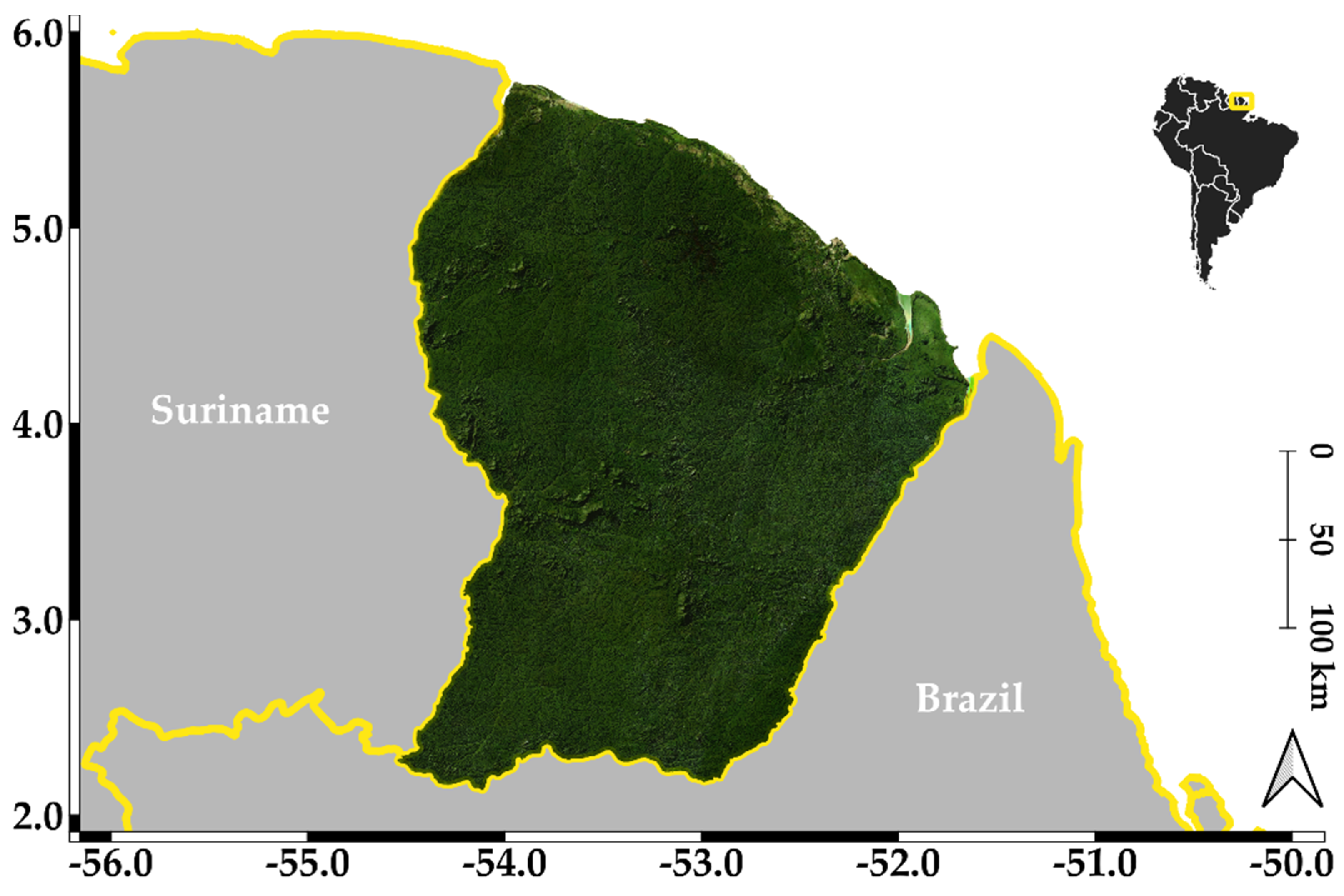
Our decision to choose a tropical forest is due to the generally dense canopy cover and tall trees, which might be limiting factors for GEDI’s lasers. In addition, the influences of beam sensitivities (the probability of a given shot over a given canopy cover reaching the ground [2]) and acquisition times on the penetration of the lasers through the canopies, or their influence on accurately detecting the tops of the canopies, will also be assessed.
The paper is organized into four sections. A description of materials and methods is given in Section 2. The results are given in Section 3, followed by the discussion and conclusions in Section 4 and Section 5.

2. Materials and Methods

2.1. Study Site

French Guiana is located on the northern coast of the South American continent and borders the Atlantic Ocean, Brazil, and Suriname (Figure 1). The study site’s area is approximately 83,500 km2, where forest covers more than 95% of the surface. The terrain is mostly flat, with 70% of slopes being less than 5°, and rises to occasional small hills and mountains, with altitudes that range from 0 to 851 m [10]. The climate, based on the Köppen−Geiger classification [11], is mainly tropical and belongs to the Am (tropical monsoon) category, with a small part in the northwest belonging to Af (tropical rainforest) category.

2.2. Datasets

2.2.1. GEDI

GEDI-collected waveforms (Level 1), as well as their processing (Level 2), are provided by NASA’s Land Processes Distributed Active Archive Center (LP DAAC). The Level 1 data product, namely the L1B data product [12] includes the geolocated waveforms as collected by the GEDI system. The Level 2 data product includes footprint-level elevation and canopy height metrics (L2A, [13]) and footprint-level canopy cover and vertical profile metrics (L2B, [14]). In this study, we extracted the geolocation (longitude, latitude, and elevation) of the received waveforms, as well as their acquisition time, from Version 2 of the L1B data product. The L2A data product processes the waveforms using six possible configurations (henceforth referred to as algorithms) of differing thresholds to satisfy a variety of acquisition scenarios [5]. Moreover, in the L2A data product, a variable named ‘selected_algorithm’ corresponds to the algorithm with the lowest (in terms of elevation) non-noise ground return (henceforth referred to as the “lowest mode”). Therefore, from L2A, we extracted the following variables derived from the processing algorithm identified by the selected_algorithm variable:
  • The latitude, longitude, and elevation of the lowest mode.
  • The latitude, longitude, and elevation of the instrument.
  • The number of detected modes (num_detectedmodes).
  • The acquisition date and time of the shot.
  • The beam sensitivity, that is, the probability of detecting the ground below a given canopy cover 90% of the time with a 5% chance of a false positive [2].
  • The viewing angle (VA) at acquisition time [15].
  • The signal-to-noise ratio (SNR) [15].
  • The relative height at 100% (RH100) of returned energy, in essence, the distance between the ground return and the canopy top.
  • The elevation of the lowest mode (ELM) and the elevation of the highest return (EHR), which represents the canopy top.
Over French Guiana, 8,662,215 shots were acquired during the period between April 2019 and August 2021. However, not all of these shots were usable due to unfavorable atmospheric conditions (e.g., clouds) that affected them. Therefore, a waveform was not investigated further if it met any of the following criteria:
  • Shots without any detected modes (num_detectedmodes = 0). These shots were noisy signals with a signal-to-noise ratio (SNR) of 0 on a linear scale.
  • Shots where the absolute difference between the elevation of the lowest mode (ELM) and the corresponding SRTM DEM was higher than 75 m ( | ELM SRM | > 75 ).
  • Incomplete waveforms, in essence, waveforms with an insufficient number of bins. These waveforms are detected by their search_end variable (end location of the usable part of the waveform) that is near the total number of bins in a waveform “rx_sample_count” (rx_sample_count—search_end ≤ 1 bin).
  • Shots where RH100 < 3 m. These shots most likely corresponded to bare soil or low vegetation.
After the filtering scheme, ~55% of shots were retained for further analysis

2.2.2. The Land, Vegetation, and Ice Sensor Data

The Land, Vegetation, and Ice Sensor (LVIS), developed by the National Aeronautics and Space Administration (NASA) [16] is an airborne, full-waveform LiDAR sensor consisting of a 1064 nm wavelength laser, with a nominal footprint diameter of 25 m. The laser fires 10 ns, 5 mJ pulses at repetition rates of up to 500 Hz. The LVIS data used in this study were acquired between 23 and 31 July 2021 over French Guiana from NASA’s Gulfstream V at an altitude of ~8 km. During this mission, around 21 million LVIS footprints were acquired over French Guiana. From the LVIS L2 elevation and height products, the following variables were extracted: The geolocation (latitude and longitude) of the detected lowest mode, as well as its elevation (ELM), the elevation of the highest return (EHR), the sensitivity, and the RH100.
Generally, LVIS data are available pre-filtered, such that data affected by questionable observational conditions are already removed. Nonetheless, to stay consistent with the filtering applied to the GEDI data, we removed all LVIS shots where the absolute difference between the ELM and SRTM was higher than 75 m. Thus, 87.9% of the shots were retained after the application of this filter.

2.2.3. Canopy Height Model

A canopy height model (CHM) over French Guiana produced by Fayad et al. [17] was used in this study for the assessment of the different GEDI laser systems. The map was created by a data fusion of spaceborne LiDAR data acquired by the geoscience laser altimeter system (GLAS) on board the Ice, Cloud, and Land Elevation Satellite (ICESat), airborne LiDAR data (covering 4/5 of French Guiana with a point density of 1.59 pts/km2), environmental (a geological map, rainfall data, and a forest landscape-types map), and optical data (MODIS). To create this map, the random forests (RF) algorithm was used to find a relationship between the airborne LiDAR canopy heights and the auxiliary data, which allowed the estimation of the canopy heights over all of French Guiana with a grid size of 250 m. Next, model residuals (reference canopy heights—RF-estimated canopy heights) were interpolated by kriging to increase the map’s precision to 3.3 m (RMSE). “Kriged model residuals” refer to the ordinary kriging of regression (RF) residuals that are assumed to present second-order stationary spatial covariance. Figure 2 shows that the distribution of canopy heights using the Fayad CHM map for each footprint from GEDI’s coverage and full-power lasers, as well as LVIS, is very similar for the three LiDAR datasets. It is worth noting that, while comparing GEDI acquisitions directly with a canopy height model could provide a better performance assessment, the available canopy height model does not have enough resolution (with a pixel size of 250 m) to be directly comparable to GEDI’s 25 m footprints. In essence, each pixel from the Fayad CHM could contain a large number of GEDI acquisitions, and given the heterogeneity of the study area, a direct comparison might not prove to be accurate.

2.3. Data Comparison

LVIS data are provided as orthometric elevations with respect to the World Geodetic System WGS84, using the Earth Gravity Model EGM96, while GEDI elevations are provided as ellipsoidal heights with respect to WGS84. Therefore, in order to make direct comparisons between LVIS and GEDI elevations, we have converted LVIS orthometric elevations to ellipsoidal elevations by removing the geoidal heights using the EGM96 geoid interpolated at each LVIS footprint location.
In order to assess the capacities of the lasers of GEDI and LVIS in their penetration within the canopies, as well as their detection of the tops of canopies, we will focus on two variables derived from the processing of GEDI’s waveforms. The variables of interest are the elevation of the detected top of the canopy, named “the elevation of the highest detected return” (EHR) and the elevation of the detected ground return, or “lowest mode” (ELM). In addition to the GEDI-derived EHR and ELM, we will also use the LVIS-derived EHR and ELM in order to assess how an instrument that is similar to GEDI performs at lower acquisition altitudes.
The assessment of both EHR and ELM values provided by the different lasers will be made against the elevations provided by the SRTM DEM, which correspond to the elevations of the scattering center within the canopy [9]. Over French Guiana, this elevation corresponds to a mean penetration distance that ranges between 2.3 and 8.5 m over densely vegetated forests [3]. However, SRTM errors are assumed to be systematic for similar canopy height ranges [3]. Next, EHR and ELM derived elevations from both LVIS and GEDI will be assessed as a function of waveform sensitivity. Finally, the penetration of GEDI shots will also be evaluated as a function of acquisition time.

3. Results

3.1. Assessment of the Lasers’ Penetration and Top-of-Canopy Detection

The results presented in Figure 3 of the elevation differences between ELM values from the coverage (C) and full-power (FP) lasers of GEDI and those from LVIS with respect to the SRTM DEM show that, for the three tested lasers, the difference increased with increasing canopy heights (CHM). Nonetheless, the elevation difference, which is a proxy of laser penetration in the canopy, was the lowest for the coverage lasers, and the highest with LVIS. Indeed, for the coverage lasers, elevation differences between the ELM and SRTM DEM decreased from a median of ~0.4 m for CHM between 5 and 7 m and reached a minimum of −7.9 ± 0.3 m for CHM > 25 m (Figure 3). For the case of the FP lasers, the difference between GEDI and SRTM elevations decreased from 0.68 m for CHM between 5 and 7 m and reached a minimum of −15.4 ± 0.1 m for CHM > 33 m (Figure 3). Finally, for LVIS, the difference (ELM—SRTM) decreased from a median of −0.8 m for CHM between 5 and 7 m and reached a minimum of −26.8 ± 0.1 m for CHM > 41 m (Figure 3). The results of the mean and standard deviation of the difference between ELM and SRTM elevations can be found in Table A1.
Regarding the difference between EHR and STRM, the results in Figure 4 show that the elevation difference between the highest detected mode from the three lasers (GEDI’s coverage and full-power lasers and LVIS) and SRTM increased with increasing canopy heights. Moreover, GEDI’s coverage lasers showed the lowest median difference which ranged from 6.1 m for CHM between 5 and 7 m to 16.9 m for CHM higher than 45 m (Figure 4). For CHM between 5 and 35 m, LVIS showed higher differences between EHR and SRTM than GEDI’s full-power lasers. However, for canopy heights higher than 35 m, the median difference between EHR and SRTM were similar for both LVIS and GEDI’s full-power lasers and ranged from 18.1 to 19.9 m (Figure 4). The results of the mean and standard deviation of the difference between EHR and SRTM elevations can be found in Table A2.

3.2. RH100 Estimates from GEDI and LVIS Acquisitions as a Function of Fayad CHM

The results of Figure 5a show that RH100 estimates from GEDI’s coverage lasers are, on average, lower than those obtained in the study of Fayad et al. [17], and this is true for all ranges of canopy heights. The bias, which represents the mean difference between the estimated RH100 from the coverage laser acquisitions and Fayad CHM, was −8.3 m. Moreover, the coverage laser was only able to estimate canopy heights, on average, of up to ~24 ± 10 m for all ranges of canopy heights higher than 30 m. The full-power lasers on the other hand showed RH100 values that were higher than those estimated by the coverage lasers (mean difference between RH100 and Fayad CHM of −1.2 m). In fact, the RH100 estimates from the full-power lasers were higher, on average, than those obtained by Fayad’s map for canopy heights between 5 and 30 m, after which the RH100 estimates from the full-power lasers remained more or less the same (ranging between 31.6 ± 10.3 m and 33.8 ± 11.5 m) for Fayad canopy height ranges between 30 and higher (Table 1). A similar trend in the full-power lasers was observed with LVIS (Figure 5c, Table 1). Nonetheless, LVIS showed higher values of RH100 in comparison to those obtained with GEDI’s full-power lasers (mean difference between LVIS-derived RH100 and Fayad CHM of 2.19 m). In fact, with LVIS, RH100 estimates ranged between 35.8 ± 9.1 m and 38.3 ± 9.6 m for canopy heights of 35 m and higher. For LVIS, the mean difference between the estimated RH100 values and Fayad CHM is 2.2 m.

3.3. Beam Sensitivity Effect on Laser Penetration and Top-of-Canopy Detection

Figure 6 shows the distribution of the beam sensitivities of GEDI’s shots from the coverage and full-power lasers, as well as the sensitivities of LVIS’s shots. For GEDI’s coverage laser, most of the shots have a sensitivity in the 96–98% range (51.7% of shots), with 59.2% of the shots having a sensitivity ≥ 96%. For GEDI’s full-power lasers, Figure 6 shows that more than half (56.2%) of the shots have a sensitivity greater than 98%, and 9.1% have a sensitivity greater than 99%. For LVIS, the majority of the shots exhibited a sensitivity greater than 99% (81.1% of the shots), with more than 91% of the shots having a sensitivity greater than 98%.
In this section, to assess the effects of shot sensitivity on the detection of the ground return and the canopy tops, we selected from GEDI’s coverage laser and full-power lasers, as well as from LVIS, all the shots with beam sensitivities greater than 98%. The results presented in Figure 7, which represent the difference between the elevation of GEDI’s or LVIS’s lowest detected mode (ELM) and the SRTM, show that, by selecting the shots with the highest beam sensitivities, an increase in this difference is observed, and this is true for both GEDI’s and LVIS’s shots. Indeed, for GEDI’s coverage lasers, the median penetration of the shots (estimated from the difference between ELM and SRTM) with sensitivities ≥ 98% increased in comparison to a collection of all the shots (Figure 3 vs. Figure 7) by 0.14 m for canopy heights in the 5–7 m range and reached a maximum of 5.5 m for canopy heights in the 45–47 m range. For GEDI’s full-power lasers, the median difference in penetration for shots with sensitivities ≥ 98% increased in comparison to a collection of all the shots (Figure 3 vs. Figure 7) by an almost-constant factor of 2.3 ± 0.8 m for all canopy height ranges. Finally, with LVIS, the median increase in penetration for shots with sensitivities ≥ 98% and a collection of all the shots was the lowest (in comparison to GEDI’s coverage or full-power lasers) with a mean increase of 0.6 ± 0.5 m (Figure 3 vs. Figure 7). The results of the mean and standard deviation of the difference between ELM and SRTM elevations for shots with sensitivities ≥ 98% can be found in Table A3.
The difference between the elevation of the highest return (EHR) and SRTM for EHR of GEDI and LVIS shots with sensitivities ≥ 98% is reported in Figure 8. Similar to the difference between ELM—SRTM, the results also indicate an increase in the difference between EHR and SRTM for the three laser types when selecting the shots with the highest sensitivities. The median difference between EHR and SRTM increased for all canopy height ranges (Fayad CHM) for the shots with sensitivity ≥ 98% in comparison to a collection of all the shots (Figure 8 vs. Figure 4). The mean increase of the median difference between EHR and SRTM is 1.9 ± 1.1 m for GEDI’s coverage laser, 2.0 ± 1.7 m for GEDI’s full-power lasers, and 0.5 ± 0.4 m for LVIS. The results of the mean and standard deviation of the difference between EHR and SRTM elevations for shots with sensitivities ≥ 98% can be found in Table A4.

3.4. GEDI- and LVIS-Derived RH100 as a Function of Fayad CHM and Sensitivity

In this section, we compared the estimated RH100 estimated from GEDI’s coverage and full-power lasers and LVIS to Fayad CHM. The results indicate that the shots from either GEDI or LVIS with sensitivity ≥ 98% have, on average, a higher estimated RH100 in comparison to a collection of all the shots (Figure 9). For GEDI’s coverage lasers, an average increase of 5.1 ± 0.9 m in the estimated RH100 was observed (Table 1 vs. Table 2). For GEDI’s full-power lasers, the increase in RH100 was slightly lower than that of the coverage lasers and averaged 4.4 ± 1.6 m (Table 1 vs. Table 2). LVIS reported the lowest increase in the estimated RH100 for shots with a sensitivity ≥ 98% in comparison to a collection of all the shots, with an average increase of 1.3 ± 0.5 m (Table 1 vs. Table 2). Moreover, for shots with a sensitivity ≥ 98%, the difference in estimated RH100 values between GEDI’s full-power laser and LVIS decreased from 4.6 ± 0.5 m to 2.3 ± 0.4 m for canopy height ranges ≥ 20 m.

3.5. Effect of Acquisition Time on Laser Penetration and Top-of-Canopy Detection

The effect of acquisition time on laser penetration (we used the elevation difference of ELM and SRTM as proxy) and on detecting the canopy tops (we used the elevation difference between EHR and SRTM as a proxy) was assessed for GEDI’s coverage lasers and full-power lasers for five time ranges. We could not assess the effect of acquisition time for the LVIS data as they were mostly acquired between 10 a.m. and 2 p.m., local time. Moreover, to reduce the uncertainties caused by shots with insufficient penetration, only acquisitions with beam sensitivity ≥ 98% were analyzed. Finally, only shots corresponding to Fayad CHM higher than 25 m were considered, given the low number of shots corresponding to Fayad CHM lower than 25 m.
The results presented in Figure 10a show that, for the coverage lasers, the median penetration (represented by the difference between ELM and SRTM) decreased to a minimum for all canopy height (Fayad CHM) ranges (i.e., a lower difference between ELM and SRTM in comparison to shots acquired at other times) for shots acquired between 8 a.m. and 12 p.m. The penetration of shots acquired after 12 p.m. then started increasing and reached a maximum for shots acquired after 4 a.m., and this was true for all canopy height ranges. For shots acquired between midnight and 8 a.m., the penetration was the highest. For the full-power lasers (Figure 10b), the penetration of the lasers did not seem to be affected by solar noise as the penetration of the lasers (i.e., the difference between ELM and SRTM) was mostly similar for all acquisition times and all canopy height ranges. The results of the mean and standard deviation of the difference between ELM and SRTM elevations for different acquisition times can be found in Table A5.
Regarding the effects of acquisition time on the detection of the tops of canopies (assessed using the difference between EHR and SRTM), the results presented in Figure 11a show that, for the coverage lasers, a small decrease in the difference between EHR and SRTM was observed for acquisitions made between 8 a.m. and 12 p.m. in comparison to acquisitions made during other times of the day. Nonetheless, for a given canopy height range (from Fayad CHM), the difference between EHR and SRTM was similar for all acquisition times. Regarding the acquisitions made by the full-power lasers, the results presented in Figure 11b show that acquisition time had no effect on the estimation of the canopy tops as the difference between EHR—SRTM was similar for all acquisition times and all canopy height ranges. The results of the mean and standard deviation of the difference between EHR and SRTM elevations for different acquisition times can be found in Table A6.

4. Discussion

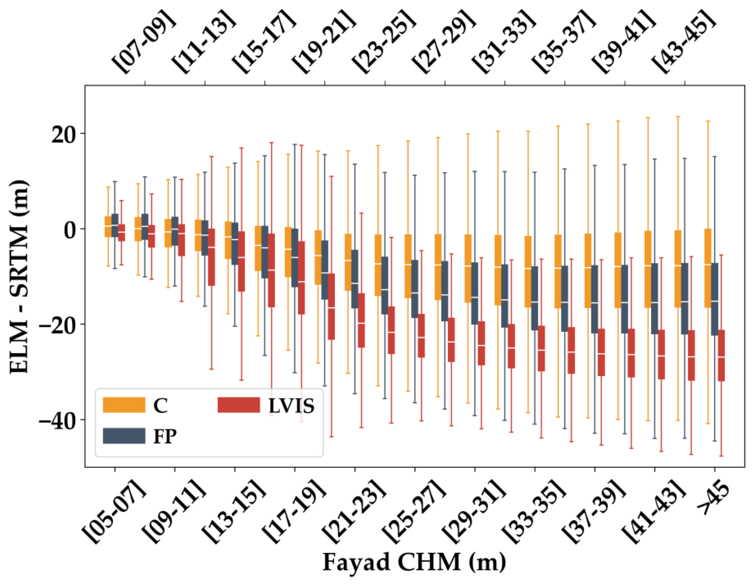
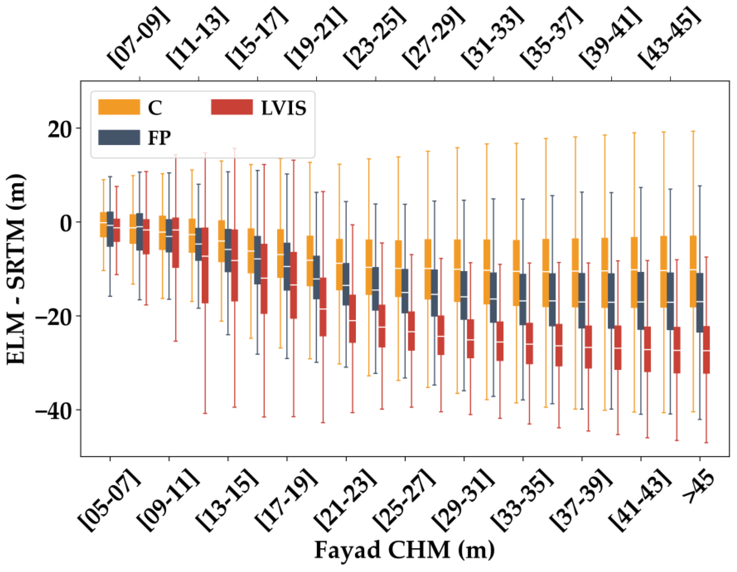
The analysis of the difference between the elevation of the lowest mode (ELM) and SRTM elevations for GEDI’s coverage and power lasers, as well as LVIS, show that both the types of GEDI’s lasers and LVIS are limited in their capability in reaching the ground in a tropical context with high canopy-cover and tall trees. Moreover, with a 5 mJ energy output per shot and ~400 km altitude, the coverage lasers are only able to reach approximately one-third of the distance into the canopy in comparison to LVIS, which is closer to Earth’s surface and using a laser with the same energy output, and this was true for all canopy height ranges. Indeed, the median difference between ELM and SRTM for GEDI’s coverage lasers was −7.9 m for trees taller than 25 m, while for LVIS, the median difference between ELM and SRTM was −24.7 m on average. In the case of the full-power lasers, which have an energy of 10 mJ per shot, the penetration into the canopy was higher than the coverage lasers (median difference of −14.8 m for trees taller than 25 m); however, it was still lower than the penetration of LVIS (−24.7 m on average). Moreover, for both GEDI’s coverage and full-power lasers, the penetration could only reach a certain depth into the canopy. For the coverage lasers, the maximum depth was reached for canopy heights of 25 m and higher, while in the case of the full-power lasers, the maximum depth was reached for canopy heights of 35 m and higher. Indeed, in the case of the coverage lasers, the median difference between ELM and SRTM for shots with Fayad CHM > 25 m is −7.9 ± 0.3 m and 85% of shots presented a difference between ELM and SRTM lower than −18.4 ± 0.3 m. In the case of the full-power lasers, the median difference between ELM–SRTM for shots with Fayad CHM > 35 m is −15.4 ± 0.12 m, and 85% of shots showed a difference between ELM and SRTM that was lower than −23.7 ± 0.41 m. Moreover, while in this study we could not directly compare GEDI footprints with corresponding airborne laser scanning data (ALS), if we compare GEDI’s lasers performance with those from LVIS for similar canopy height ranges, we can note that both GEDI’s lasers are underperforming over highly, densely vegetated forests in comparison to LVIS. This finding is in contrast to previous studies that assessed the penetrative capabilities of spaceborne full-waveform LiDAR systems. For example, the study by Chen [18], conducted over a study area in South Carolina using ICESat data, found a mean difference of −0.97 m. Next, the studies by Hilbert and Schmullius [19] and the study by Adam et al. [4], using, respectively, ICESat and GEDI data, over a study area in the Thuringian forest, found a difference between LiDAR-waveform-derived ground return and ALS data of, respectively, a 0.19 m (mean difference) and a 0.18 m (median difference). Finally, while not analyzed in this article, acquisition dates could also effect the penetrative capabilities of GEDI. In this study, some GEDI acquisitions had higher penetration than others. Some studies reported that rainfall could have an effect on penetration [20]. However, this was not the case over our study area, and since the effects of the acquisition dates were similar for both the coverage and full-power lasers, the most probable explanation would be the loss of leaves during certain seasons, allowing the lasers to better penetrate into canopies.
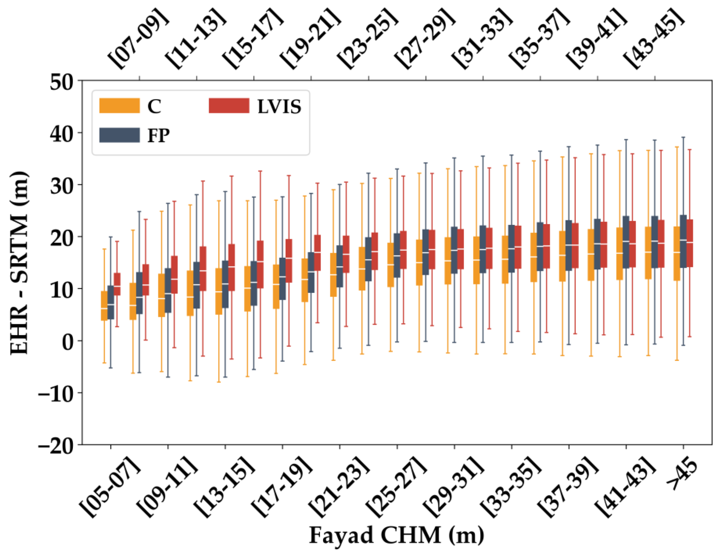
Regarding the detection of the tops of canopies, both of GEDI’s lasers also show some limitations in the detection of canopy tops in comparison to LVIS. However, given the full-power lasers’ higher energy-per-shot in comparison to the coverage lasers, GEDI’s full-power lasers were better able to detect canopy tops. Moreover, the median difference between EHR–SRTM for GEDI’s full-power lasers and LVIS are in accordance with the literature. In fact, for Fayad CHM between 25 and 35 m, the median difference of EHR–SRTM was around 1 m, after which the difference between EHR–SRTM from GEDI’s full-power lasers and LVIS decreased to around 0.3 m. These findings were found to be similar to those of comparable studies (e.g., [4,19,21,22]). Nonetheless, while some studies reported negative differences between full-waveform-derived canopy tops and canopy tops derived from ALS data (i.e., waveform-derived canopy tops are lower than ALS-based ones) (e.g., [21,22]) while the others reported positive differences (e.g., [4,19]), the findings in this study (EHR from GEDI is lower in general than EHR from LVIS) are logical, given the fact that both GEDI and LVIS are full-waveform lasers with similar specifications. Moreover, the detection of the canopy tops using either GEDI’s coverage lasers or the full-power lasers is linked to the canopy cover. Indeed, while the difference between the elevation of the highest return (EHR) and SRTM was lower for both GEDI’s coverage and full-power lasers than the differences reported using LVIS for all canopy height ranges from Fayad CHM, this difference decreased with an increase in canopy heights. This is because, on average, taller trees have higher canopy cover, therefore increasing the canopy surface over which the lasers can reflect off.
The detection of both the canopy tops and ground return is affected by two variables, the energy of the reflected pulse as well as the chosen thresholds used to detect the canopy-top and ground returns from each waveform. Therefore, by selecting the footprints with sensitivities higher than 98%, which in essence means that ground return is detected for canopy cover up to 98% [2], both the penetration and detection of canopy tops seem to improve for these selected shots. Indeed, for shots with beam sensitivities ≥ 98%, the estimated 
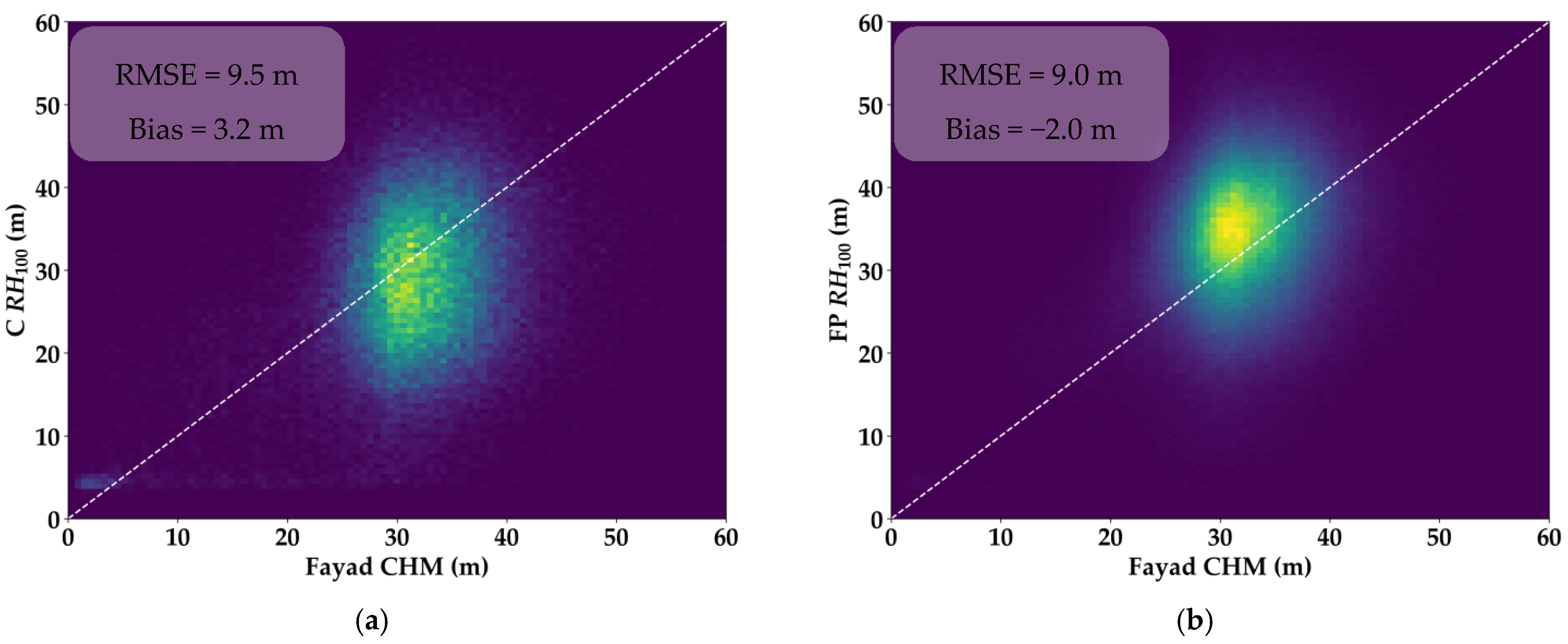
RH100, which is the difference between the elevation of the ground return and the elevation of the canopy top, is increased, on average, by 5 m for both the coverage lasers and the full-power lasers. Nonetheless, in the case of the coverage laser, the average of estimated RH100 values ( R H 100 ¯ = 28.8 m) was still lower than the RH100 estimates from both the full-power lasers ( R H 100 ¯ = 34.1 m) and LVIS ( R H 100 ¯ = 35.9 m). Moreover, by selecting only the shots with the best probabilities of reaching the ground (i.e., shots with beam sensitivities ≥ 98%), more than 64% of coverage laser shots were removed, as were close to 41% of the full-power laser shots. Finally, even by selecting the GEDI and LVIS shots with sensitivity ≥ 98%, respectively, 62.7%, 38.8%, and 29.7% of shots from GEDI’s coverage laser, GEDI’s full-power lasers, and LVIS have RH100 estimates that are lower than the values from the corresponding Fayad CHM estimates (by −8.63 ± 6.2 m, −6.6 ± 5.6, and −6.8 ± 6.2 m, on average, for, respectively, the coverage, full-power, and LVIS). For these shots (GEDI and LVIS shots with lower RH100 estimates than Fayad CHM), this is a clear indicator of underestimation [23], given the fact that RH100 is a measure of the maximum canopy height, while Fayad CHM is the average of maximum canopy heights over a 250 m2 area. These findings are different from the literature that stipulates that a beam sensitivity of 98% should be enough to detect the ground with a tree cover of 98% or less. However, over our study area, the mean tree cover reported from the L2B dataset was around 85%. Therefore, in a forest with very tall trees and dense vegetation, the detection of the ground return could be problematic, even with acquired shots with very high sensitivities.
Regarding the effects of the selected algorithm (a1 to a6) on the detection of canopy tops and ground return, in this study, the elevation of these two variables (ground and tops of canopies) was estimated based on the suggested algorithm to use from the ‘selected_algorithm’ variable in the L2A data product. The ‘selected_algorithm’ provides the algorithm detected as producing the lowest non-noisy ground return. Nonetheless, over our study area, the ‘selected_algorithm’ suggested only either a1 (back threshold of 6 ns) or a2 (back threshold of 3 ns). Choosing the appropriate back threshold is primordial for the detection of the ground return, especially over densely vegetated areas where the reflection off of the ground is very weak. As such, by choosing a high back threshold value, the weak ground return will not be detected, and canopy heights will thus be underestimated. Over French Guiana, both a1 and a2 seem to be inadequate for the processing of the waveforms, especially those acquired by the coverage lasers. Therefore, to potentially detect very weak ground returns, a possible solution would be to choose a back threshold with a lower value than those of algorithms a1 or a2. Nonetheless, the choice of a lower-valued back threshold could have the adverse effect of incorrectly detecting high noise as the ground return [4], which might lead to over-estimating canopy heights. Obtaining the correct values of thresholds is still an issue with full-waveform-based LiDAR sensors as they could be different from one area to another, and the reliance on the best settings group from the ‘selected_algorithm’ is not enough.
The effects of acquisition time on the detection of the ground return indicate that the coverage lasers are affected by solar noise, given that acquisitions made between 8 a.m. and 4 p.m. have the lowest elevation differences between ELM and SRTM (i.e., less penetration) than acquisitions made at other times of the day. This effect was not present for the full-power lasers, which showed, on average, similar penetration values for all acquisitions. The results concerning the effects of solar noise on the detection of the ground return are consistent with the findings of Adam et al. [4]. However, in their study, they reported that beam type has no influence on DTM accuracy for forests with low-density cover, which is not the case for forests with high-density cover, such as the forest from this study area where the full-power lasers perform better.
The effects of solar noise on the detection of canopy tops seem to slightly affect the coverage lasers as the coverage lasers reported slightly lower elevation differences between EHR and SRTM for acquisitions made between 8 a.m. and 12 p.m. in comparison to acquisitions made during other hours. These findings are different from what was obtained in the study by Adam et al. [4], where they found that the effects of solar noise on the accuracy of canopy tops and ground return detection were similar. The discrepancies between their study and ours could be explained by the differences in tree densities between the two study sites. Indeed, our study site is characterized by a high-density cover throughout, indicating that both the coverage and full-power lasers have enough surface area from canopy tops to reflect, thus minimizing the effects of solar noise.

5. Conclusions

The results presented in this study show that, even after the application of different filters to remove unusable GEDI acquisitions, the remaining shots acquired by the coverage and full-power lasers were limited in their capabilities to reach the ground over tropical forests. This result is quite different from comparable studies that analyzed the accuracy of GEDI over temperate forests, for example. Indeed, previous studies saw a sub-meter DTM difference between GEDI and reference ALS data, while in this study, a difference of several meters was observed between the difference of the ground elevation from GEDI’s lasers and SRTM and the difference between the ground elevation from LVIS and SRTM. Moreover, the analysis showed that the coverage lasers could potentially only be used to estimate canopy heights in the 20–30 m range.
The analysis of beam sensitivity showed results that are similar to comparable studies. In essence, GEDI-acquired shots with higher sensitivity have a higher probability of reaching the ground than shots with lower sensitivity. Nonetheless, our findings indicate that, in a tropical context, GEDI’s lasers could still not reach the ground for certain shots, even with beam sensitivities higher than 98% and a significantly lower canopy cover percentage.
Regarding the detection of canopy tops, both GEDI lasers showed a lower median difference between detected top-of-canopy and SRTM DEM elevations in comparison to LVIS, especially for trees with heights lower than 25 m. Moreover, similar to previous findings, the coverage lasers showed fewer capabilities than the full-power lasers.
One possible improvement on the accuracy of the detected ground return and canopy tops would be choosing lower forward and backward thresholds in the algorithm settings groups than the ones suggested by the ‘selected_alrogithm’ in the L2A dataset. However, selecting a very low threshold, especially for ground detection, could also introduce uncertainties as the algorithm could incorrectly detect noise as the ground return.
Finally, acquisition time also showed some effects on the detection of ground return and canopy tops for GEDI’s coverage lasers. Indeed, shots acquired in the early morning or the late afternoon showed slightly better capabilities at detecting both surfaces. This result is similar to that of comparable studies.

Author Contributions

Conceptualization, I.F. and N.B.; methodology, I.F. and N.B.; software, I.F.; validation, I.F., N.B. and K.L.; formal analysis, I.F., N.B. and K.L.; data curation, I.F. and K.L.; writing—original draft preparation, I.F. and N.B.; writing—review and editing, K.L.; visualization, I.F. All authors have read and agreed to the published version of the manuscript.

Funding

This research received funding from the French Space Study Center (CNES, TOSCA 2022 project) and the National Research Institute for Agriculture, Food and the Environment (INRAE).

Data Availability Statement

GEDI data were downloaded from the Land Processeses Distributed Active Archive Center (LP-DAAC, https://lpdaac.usgs.gov, accessed on 16 June 2022). LVIS data were downloaded from the National Snow and Ice Data Center (NSIDC, https://nsidc.org, accessed on 16 June 2022).

Acknowledgments

The authors would like to thank the GEDI team and the NASA LPDAAC (Land Processes Distributed Active Archive Center) for providing the GEDI data.

Conflicts of Interest

The authors declare that they have no known competing financial interests or personal relationships that could have appeared to influence the work reported in this paper.

Appendix A

Table A1. Mean (M) and standard deviation (SD) in meters of the elevation difference between ELM and SRTM. (C) and (FP) correspond to the ELM values from GEDI’s coverage and full-power lasers, respectively. (LVIS) corresponds to the ELM values from LVIS.
Fayad CHM (m)
5–1010–1515–2020–2525–3030–3535–4040–45>45
MSDMSDMSDMSDMSDMSDMSDMSDMSD
C−0.44.7−2.16.0−5.07.4−7.48.6−8.19.5−8.810.3−8.911.0−8.611.5−8.012.0
FP−0.45.4−2.86.5−6.58.0−11.28.5−12.99.3−14.010.0−14.610.6−14.611.1−14.511.3
LVIS−2.86.6−7.09.14−12.110.1−20.08.5−22.77.9−24.28.2−25.28.5−26.08.9−26.59.1
Table A2. Mean (M) and standard deviation (SD) of the elevation difference between EHR and SRTM. (C) and (FP) correspond to the EHR values from GEDI’s coverage and full-power lasers, respectively. (LVIS) corresponds to the EHR values from LVIS.
Fayad CHM (m)
5–1010–1515–2020–2525–3030–3535–4040–45>45
MSDMSDMSDMSDMSDMSDMSDMSDMSD
C7.75.89.46.410.56.913.07.514.97.515.47.816.08.216.58.616.68.9
FP8.77.010.76.711.86.914.97.617.07.917.68.218.88.618.88.819.38.8
LVIS12.94.514.66.616.36.717.96.218.36.318.66.719.07.019.37.319.67.6

Appendix B

Table A3. Mean (M) and standard deviation (SD) in meters of the elevation difference between ELM and SRTM for shots with a sensitivity ≥ 98%. (C) and (FP) correspond to the ELM values from GEDI’s coverage and full-power lasers, respectively. (LVIS) corresponds to the ELM values from LVIS.
Fayad CHM (m)
5–1010–1515–2020–2525–3030–3535–4040–45>45
MSDMSDMSDMSDMSDMSDMSDMSDMSD
C−1.35.3−3.66.1−6.67.5−10.08.2−11.58.8−12.69.4−13.49.8−13.110.2−12.911.1
FP−2.76.4−5.76.6−9.77.3−13.67.2−15.07.9−16.18.6−16.69.1−16.89.6−20.09.8
LVIS−3.27.1−8.09.6−13.49.9−20.78.0−23.57.2−25.07.4−25.97.9−26.58.2−26.88.6
Table A4. Mean (M) and standard deviation (SD) in meters of the elevation difference between EHR and SRTM for shots with a sensitivity ≥ 98%. (C) and (FP) correspond to the ELM values from GEDI’s coverage and full-power lasers, respectively. (LVIS) corresponds to the ELM values from LVIS.
Fayad CHM (m)
5–1010–1515–2020–2525–3030–3535–4040–45>45
MSDMSDMSDMSDMSDMSDMSDMSDMSD
C10.35.612.75.312.75.915.26.916.57.316.77.417.27.618.08.118.28.8
FP13.86.214.15.514.65.816.76.418.27.218.67.619.27.919.88.220.08.2
LVIS13.65.015.86.217.36.318.35.818.76.018.96.419.36.819.67.1119.97.4

Appendix C

Table A5. Mean (M) and standard deviation (SD) in meters of the elevation difference between ELM and SRTM, grouped by different acquisition times and Fayad CHM. (C) and (FP) correspond to the ELM values from GEDI’s coverage and full-power lasers, respectively.
Fayad CHM (m)
25–3030–3535–40>40
ATMSDMSDMSDMSD
C[00–04]−12.98.2−13.58.6−14.29.0n/an/a
[04–08]−11.99.3−13.09.2−13.29.7−13.410.9
[08–12]−8.89.3−9.99.5−10.010.2n/an/a
[12–16]−10.99.1−11.59.6−12.09.9n/an/a
[16–20]−11.18.9−12.79.9−13.810.0−13.210.6
FP[00–04]−15.07.6−15.88.1−16.08.6−16.59.0
[04–08]−14.88.3−16.19.0−16.89.8−17.010.6
[08–12]−14.88.1−15.68.5−15.99.2−16.39.7
[12–16]−14.78.0−15.98.7−16.69.2−17.09.5
[00–04]−15.07.9−16.29.0−17.09.4−17.19.6
Table A6. Mean (M) and standard deviation (SD) in meters of the elevation difference between EHR and SRTM, grouped by different acquisition times and Fayad CHM. (C) and (FP) correspond to the ELM values from GEDI’s coverage and full-power lasers, respectively.
Fayad CHM (m)
25–3030–3535–40>40
ATMSDMSDMSDMSD
C[00–04]15.97.316.77.017.47.3n/an/a
[04–08]15.68.016.16.916.97.417.68.6
[08–12]15.37.115.67.116.27.7n/an/a
[12–16]15.87.216.27.516.47.6n/an/a
[16–20]17.17.517.38.117.78.219.18.8
FP[00–04]18.87.519.38.020.38.820.88.9
[04–08]18.08.518.58.419.18.819.79.3
[08–12]17.76.818.37.018.97.319.57.7
[12–16]18.36.718.67.118.87.419.77.6
[00–04]18.57.118.97.919.48.220.28.2

References

  1. Sun, G.; Ranson, K.; Kimes, D.; Blair, J.; Kovacs, K. Forest Vertical Structure from GLAS: An Evaluation Using LVIS and SRTM Data. Remote Sens. Environ. 2008, 112, 107–117. [Google Scholar] [CrossRef]
  2. Hancock, S.; Armston, J.; Hofton, M.; Sun, X.; Tang, H.; Duncanson, L.I.; Kellner, J.R.; Dubayah, R. The GEDI Simulator: A Large-Footprint Waveform Lidar Simulator for Calibration and Validation of Spaceborne Missions. Earth Space Sci. 2019, 6, 294–310. [Google Scholar] [CrossRef] [PubMed]
  3. Bourgine, B.; Baghdadi, N. Assessment of C-Band SRTM DEM in a Dense Equatorial Forest Zone. Comptes Rendus Geosci. 2005, 337, 1225–1234. [Google Scholar] [CrossRef]
  4. Adam, M.; Urbazaev, M.; Dubois, C.; Schmullius, C. Accuracy Assessment of GEDI Terrain Elevation and Canopy Height Estimates in European Temperate Forests: Influence of Environmental and Acquisition Parameters. Remote Sens. 2020, 12, 3948. [Google Scholar] [CrossRef]
  5. Dubayah, R.; Blair, J.B.; Goetz, S.; Fatoyinbo, L.; Hansen, M.; Healey, S.; Hofton, M.; Hurtt, G.; Kellner, J.; Luthcke, S.; et al. The Global Ecosystem Dynamics Investigation: High-Resolution Laser Ranging of the Earth’s Forests and Topography. Sci. Remote Sens. 2020, 1, 100002. [Google Scholar] [CrossRef]
  6. Duda, D.P.; Spinhirne, J.D.; Eloranta, E.W. Atmospheric Multiple Scattering Effects on GLAS Altimetry. I. Calculations of Single Pulse Bias. IEEE Trans. Geosci. Remote Sens. 2001, 39, 92–101. [Google Scholar] [CrossRef]
  7. Yang, W.; Ni-Meister, W.; Lee, S. Assessment of the Impacts of Surface Topography, off-Nadir Pointing and Vegetation Structure on Vegetation Lidar Waveforms Using an Extended Geometric Optical and Radiative Transfer Model. Remote Sens. Environ. 2011, 115, 2810–2822. [Google Scholar] [CrossRef]
  8. Hancock, S.; McGrath, C.; Lowe, C.; Davenport, I.; Woodhouse, I. Requirements for a Global Lidar System: Spaceborne Lidar with Wall-to-Wall Coverage. R. Soc. Open Sci. 2021, 8, 211166. [Google Scholar] [CrossRef] [PubMed]
  9. Sarabandi, K.; Lin, Y.-C. Simulation of Interferometric SAR Response for Characterizing the Scattering Phase Center Statistics of Forest Canopies. IEEE Trans. Geosci. Remote Sens. 2000, 38, 115–125. [Google Scholar] [CrossRef] [Green Version]
  10. Guitet, S.; Cornu, J.-F.; Brunaux, O.; Betbeder, J.; Carozza, J.-M.; Richard-Hansen, C. Landform and Landscape Mapping, French Guiana (South America). J. Maps 2013, 9, 325–335. [Google Scholar] [CrossRef] [Green Version]
  11. Peel, M.C.; Finlayson, B.L.; McMahon, T.A. Updated World Map of the Köppen-Geiger Climate Classification. Hydrol. Earth Syst. Sci. 2007, 11, 1633–1644. [Google Scholar] [CrossRef] [Green Version]
  12. Dubayah, R.; Luthcke, S.; Blair, J.; Hofton, M.; Armston, J.; Tang, H. GEDI L1B Geolocated Waveform Data Global Footprint Level V002. 2021. Available online: https://lpdaac.usgs.gov/products/gedi01_bv002 (accessed on 16 June 2022).
  13. Dubayah, R.; Hofton, M.; Blair, J.B.; Armston, H.; Tang, H.; Luthcke, S. GEDI L2A Elevation and Height Metrics Data Global Footprint Level V002. 2021. Available online: https://lpdaac.usgs.gov/products/gedi02_av002 (accessed on 16 June 2022).
  14. Dubayah, R.; Tang, H.; Armston, J.; Luthcke, S.; Hofton, M.; Blair, J. GEDI L2B Canopy Cover and Vertical Profile Metrics Data Global Footprint Level V002. 2021. Available online: https://lpdaac.usgs.gov/products/gedi02_bv002 (accessed on 16 June 2022).
  15. Fayad, I.; Baghdadi, N.; Frappart, F. Comparative Analysis of GEDI’s Elevation Accuracy from the First and Second Data Product Releases over Inland Waterbodies. Remote Sens. 2022, 14, 340. [Google Scholar] [CrossRef]
  16. Blair, J.B.; Rabine, D.L.; Hofton, M.A. The Laser Vegetation Imaging Sensor: A Medium-Altitude, Digitisation-Only, Airborne Laser Altimeter for Mapping Vegetation and Topography. ISPRS J. Photogramm. Remote Sens. 1999, 54, 115–122. [Google Scholar] [CrossRef]
  17. Fayad, I.; Baghdadi, N.; Bailly, J.-S.; Barbier, N.; Gond, V.; Hérault, B.; El Hajj, M.; Fabre, F.; Perrin, J. Regional Scale Rain-Forest Height Mapping Using Regression-Kriging of Spaceborne and Airborne LiDAR Data: Application on French Guiana. Remote Sens. 2016, 8, 240. [Google Scholar] [CrossRef] [Green Version]
  18. Chen, Q. Assessment of Terrain Elevation Derived from Satellite Laser Altimetry over Mountainous Forest Areas Using Airborne Lidar Data. ISPRS J. Photogramm. Remote Sens. 2010, 65, 111–122. [Google Scholar] [CrossRef]
  19. Hilbert, C.; Schmullius, C. Influence of Surface Topography on ICESat/GLAS Forest Height Estimation and Waveform Shape. Remote Sens. 2012, 4, 2210–2235. [Google Scholar] [CrossRef] [Green Version]
  20. Bretar, F.; Chauve, A.; Mallet, C.; Jutzi, B. Managing Full Waveform LIDAR Data: A Challenging Task for the Forthcoming Years. In Proceedings of the ISPRS Congress 2008, Beijing, China, 3–11 July 2008. [Google Scholar]
  21. Nie, S.; Wang, C.; Zeng, H.; Xi, X.; Xia, S. A Revised Terrain Correction Method for Forest Canopy Height Estimation Using ICESat/GLAS Data. ISPRS J. Photogramm. Remote Sens. 2015, 108, 183–190. [Google Scholar] [CrossRef]
  22. Popescu, S.C.; Zhao, K.; Neuenschwander, A.; Lin, C. Satellite Lidar vs. Small Footprint Airborne Lidar: Comparing the Accuracy of Aboveground Biomass Estimates and Forest Structure Metrics at Footprint Level. Remote Sens. Environ. 2011, 115, 2786–2797. [Google Scholar] [CrossRef]
  23. Sawada, Y.; Suwa, R.; Jindo, K.; Endo, T.; Oki, K.; Sawada, H.; Arai, E.; Shimabukuro, Y.E.; Celes, C.H.S.; Campos, M.A.A.; et al. A New 500-m Resolution Map of Canopy Height for Amazon Forest Using Spaceborne LiDAR and Cloud-Free MODIS Imagery. Int. J. Appl. Earth Obs. Geoinf. 2015, 43, 92–101. [Google Scholar] [CrossRef] [Green Version]
Figure 1. Location of the study site.
Remotesensing 14 02969 g001
Figure 2. Distribution of canopy heights from Fayad’s map over GEDI’s coverage (“C”), and full-power (“FP”) laser footprints, and LVIS footprints.
Remotesensing 14 02969 g002
Figure 3. Boxplots of the difference between the elevation of each waveform’s lowest mode (ELM) and SRTM from GEDI’s coverage (C) and full-power (FP) lasers, as well as those from LVIS.
Remotesensing 14 02969 g003
Figure 4. Boxplots of the difference between the elevation of each waveform’s highest return (EHR) and SRTM from GEDI’s coverage (C) and full-power (FP) lasers, as well as those from LVIS.
Remotesensing 14 02969 g004
Figure 5. RH100 estimates from GEDI’s coverage (C RH100, a) and full-power (FP RH100, b) lasers, as well as those from LVIS (LVIS RH100, c) as a function of Fayad CHM.
Remotesensing 14 02969 g005
Figure 6. Distribution of GEDI’s coverage (C) and full-power (FP) shots, as well as those of LVIS, by footprint sensitivity.
Remotesensing 14 02969 g006
Figure 7. Boxplots of the difference between the elevation of each waveform’s lowest mode (ELM) and SRTM from GEDI’s coverage (C) and full-power (FP) lasers, as well as those from LVIS. Only waveforms with sensitivity ≥ 98% were selected.
Remotesensing 14 02969 g007
Figure 8. Boxplots of the difference between the elevation of each waveform’s highest return (EHR) and SRTM from GEDI’s coverage (C) and full-power (FP) lasers, as well as those from LVIS. Only waveforms with sensitivity ≥ 98% were selected.
Remotesensing 14 02969 g008
Figure 9. RH100 estimates of waveforms with sensitivity ≥ 98% from GEDI’s coverage (C RH100, a) and full-power lasers (FP RH100, b), as well as those from LVIS (LVIS RH100, c) as a function of Fayad CHM.
Remotesensing 14 02969 g009aRemotesensing 14 02969 g009b
Figure 10. Boxplots of the difference between the elevation of each waveform’s lowest mode (ELM) and SRTM from GEDI’s coverage (a) and full-power lasers (b) as a function of acquisition time. Only acquisitions with beam sensitivity ≥ 98% were used. The lack of boxplots in (a) corresponds to the insufficiency of available data in the corresponding time ranges.
Remotesensing 14 02969 g010
Figure 11. Boxplots of the difference between the elevation of each waveform’s highest return (EHR) and SRTM from GEDI’s coverage (a) and full-power lasers (b) as a function of acquisition time. Only acquisitions with beam sensitivity ≥ 98% were used. The lack of boxplots in (a) corresponds to the insufficiency of available data in the corresponding time ranges.
Remotesensing 14 02969 g011
Table 1. Mean (M) and standard deviation (SD) in meters of the estimated RH100. (C) and (FP) correspond to the RH100 values from GEDI’s coverage and full-power lasers, respectively. (LVIS) corresponds to the RH100 values from LVIS.
Fayad CHM (m)
5–1010–1515–2020–2525–3030–3535–4040–45>45
MSDMSDMSDMSDMSDMSDMSDMSDMSD
C RH1008.16.811.58.215.59.220.49.423.09.324.19.425.09.725.19.924.710.1
FP RH1009.18.213.59.518.310.726.110.729.910.331.610.332.810.633.310.833.710.9
LVIS RH1008.79.314.612.421.412.930.710.334.09.135.89.137.29.338.29.339.49.5
Table 2. Mean (M) and standard deviation (SD) in meters of the estimated RH100 for waveforms with sensitivity ≥ 98%. (C) and (FP) correspond to the RH100 values from GEDI’s coverage and full-power lasers, respectively. (LVIS) corresponds to the RH100 values from LVIS.
Fayad CHM (m)
5–1010–1515–2020–2525–3030–3535–4040–45>45
MSDMSDMSDMSDMSDMSDMSDMSDMSD
C RH10011.77.816.37.919.38.625.28.828.08.329.38.330.58.531.18.631.48.1
FP RH10016.59.219.88.324.38.730.38.133.27.934.77.935.88.236.68.537.48.4
LVIS RH1009.89.916.812.623.712.232.09.335.28.036.97.938.28.239.28.440.38.6
Publisher’s Note: MDPI stays neutral with regard to jurisdictional claims in published maps and institutional affiliations.

