Abstract
Bohai Sea ice creates obstacles for maritime navigation and offshore activities. A better understanding of ice conditions is valuable for sea-ice management. The evolution of 67 years of seasonal ice thickness in a coastal region (Yingkou) in the Northeast Bohai Sea was simulated by using a snow/ice thermodynamic model, using local weather-station data. The model was first validated by using seasonal ice observations from field campaigns and a coastal radar (the season of 2017/2018). The model simulated seasonal ice evolution well, particularly ice growth. We found that the winter seasonal mean air temperature in Yingkou increased by 0.33 °C/decade slightly higher than air temperature increase (0.27 °C/decade) around Bohai Sea. The decreasing wind-speed trend (0.05 m/s perdecade) was a lot weaker than that averaged (0.3 m/s per decade) between the early 1970s and 2010s around the entire Bohai Sea. The multi-decadal ice-mass balance revealed decreasing trends of the maximum and average ice thickness of 2.6 and 0.8 cm/decade, respectively. The length of the ice season was shortened by 3.7 days/decade, and ice breakup dates were advanced by 2.3 days/decade. All trends were statistically significant. The modeled seasonal maximum ice thickness is highly correlated (0.83, p < 0.001) with the Bohai Sea Ice Index (BoSI) used to quantify the severity of the Bohai Sea ice condition. The freezing-up date, however, showed a large interannual variation without a clear trend. The simulations indicated that Bohai ice thickness has grown continuously thinner since 1951/1952. The time to reach 0.15 m level ice was delayed from 3 January to 21 January, and the ending time advanced from 6 March to 19 February. There was a significant weakening of ice conditions in the 1990s, followed by some recovery in 2000s. The relationship between large-scale climate indices and ice condition suggested that the AO and NAO are strongly correlated with interannual changes in sea-ice thickness in the Yingkou region.
1. Introduction
Sea ice is an important part of the Earth environment. Sea-ice-mass balance has a profound impact on the ocean, the atmosphere, and the climate [1,2]. For example, when sea ice is formed, the energy exchange between seawater and the atmosphere is significantly reduced, which, in turn, alters the energy balance of the upper ocean. Therefore, sea ice can act as a proxy, reflecting the regional and global climate [3]. The Bohai Sea is partially covered by sea ice during the winter. It is a southernmost sea with seasonal ice cover in the northern hemisphere. The seasonal sea-ice cover in the Bohai Sea has important ecological, social, and economy impacts [4,5]. Accurate long-term knowledge on ice conditions is critical for maritime operations, such as optimization and planning of ship routing in the harbors and ice-breaking operations along the ship routes.
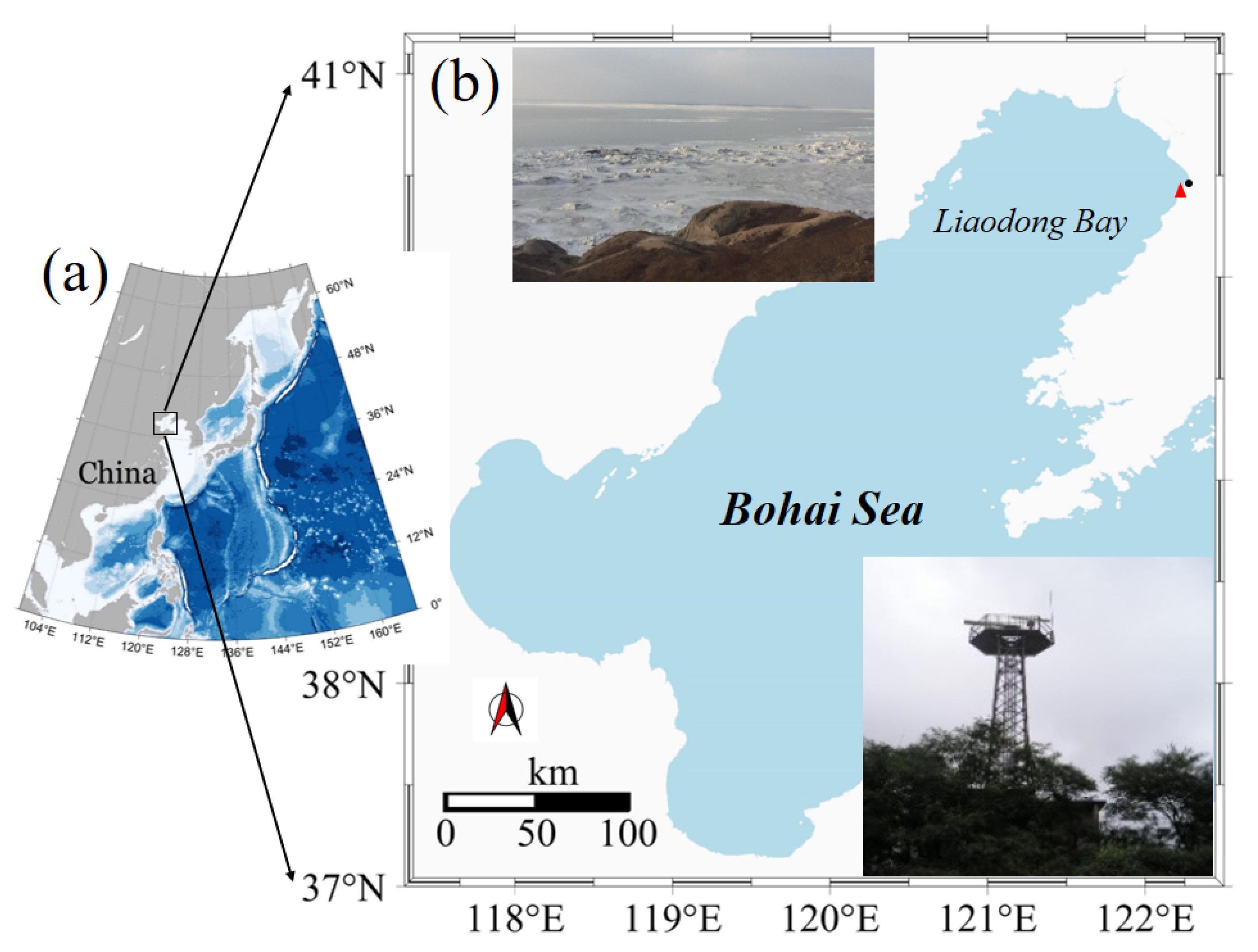
The Bohai Sea is located between north latitude (37°07′~40°56′) and east longitude (117°33′~122°08′). The maximum width of the east and west of the Bohai Sea is 346 km, and the maximum length of the south and north is 550 km (Figure 1). The costal line is roughly 3800 km in total. The sea area is 80,000 square kilometers, with an average depth of about 18 m. Bohai is a semi-enclosed sea. The sea salinity is between 29‰ and 31‰. Bohai is designated a mid-latitude sea. Meteorological parameters, such as air temperature, showed a strong seasonal cycle. The wind pattern showed typical monsoon characteristics, with an average wind speed of about 3~6 m/s and a majority NW distribution. The irregular semidiurnal M2 120 cm tide prevails. During winter, the local weather pattern is largely dominated by the high pressure in North Siberia; the low air temperature, accompanied by a strong northwest wind result, showed clear sky conditions. The sea ice is largely distributed in the Northernmost Liaodong Bay of the Bohai Sea (cf. Figure 1). The ice conditions showed large temporal and spatial distributions in Liaodong Bay. The east coast of Liaodong Bay first shows ice formations, followed by the west coast. In the normal ice winter, the maximum area of sea ice in Liaodong Bay can reach 1.8 × 10⁴ square kilometers; the distance between the open-water ice edge and coastline is about 120–166 km, and the maximum level ice thickness is about 30–40 cm [6]. In contrast with other regional seas (e.g., Baltic Sea), the long-term quantitative sea-ice observation in the Bohai Sea was insufficient; however, qualitative sea-ice documentation has a long history [7]. Remote sensing has played an important role in sea-ice observations. This technique has also been used for Bohai Sea ice investigation [8,9]. Efforts have been made to combine remote-sensing observations, operational weather forecasts, and numerical sea ice models to estimate sea-ice parameters [10].

Figure 1.
Geographical location of the Bohai Sea in the east coast of China in (a) and Liaodong Bay in the northern part of the Bohai Sea (b). The black dot (●) is the Yingkou meteorological weather station, and the red triangle is the Bayuquan coastal radar position. The in situ observation was 4 km north of the Bayuquan coastal radar position. The top image is the Bayuquan coastal landfast ice, and the bottom right photo is the coastal radar. The distance between Yingkou meteorological weather station and Bayuquan coastal radar position is 10 km.
A lot of studies have been carried out on the Bohai Sea ice, but most of them have targeted the seasonal and annual cycles. For example, to observe sea-ice thickness in Liaodong Bay, MODIS data were applied to monitor the spatiotemporal evolution of Bohai sea ice [11,12,13], and a semi-empirical model based on hyperspectral remote sensing was developed to calculate seasonal ice thickness [14,15]. Few studies have focused on long-term ice conditions in the Bohai Sea by investigating the large-scale climate index, e.g., the Arctic Oscillation (AO), local temperature, and their linkages to the Bohai Sea ice conditions [16,17]. A recent study [18] focused on the long-term variability in the Bohai Sea ice area by using a statistical method. Understanding changes in long-term ice conditions would require long-term sustainable in situ observations; such an undertaking would be a big challenge in the Bohai Sea. The sea-ice process model can be used to tackle this challenge. Modeling results are based on sea-ice physics and have a strong connection with weather and climate forcing condition. If the model is validated and weather data are reliable, we may expect that the results from the physical-based ice model would provide valuable insights into long-term ice conditions that would potentially be useful for the design and construction of coastal and offshore constructions and ice management for ship navigations. A physical long-term investigation of Bohai Sea ice is still missing. There are long-term meteorological observations around the Bohai Sea. The local long-term ice conditions can be reconstructed by using a well-validated physical ice model.
In this study, we carried out long-term ice-thickness modeling by using a high-resolution thermodynamic snow-and-ice model (HIGHTSI) forced by weather station data observed in Yingkou, north of the Bohai Sea. A multi-decadal sea-ice-mass balance time series was calculated. In the coastal region, the ice-mass balance is mainly driven by thermodynamic processes [19]. We investigate modeled sea-ice parameters, particularly the time series of ice thickness, freeze-up and breakup dates, and their interannual variations.
The objective of this study was to find the meteorological-driven interannual coastal sea-ice-mass balance and its linkages with climate change in the region. Our results are compared with previous Bohai Sea ice studies. The modeled ice parameters can be useful for the Bohai Sea ice remote sensing and have potential applications for other seasonal ice-covered seas [19,20].
2. Data and Methods
2.1. Study Site
Sea-ice conditions in the Bohai Sea respond to global climate change [5]. Ice exists in the Liaodong Bay (Figure 1) every winter season. Liaodong Bay has the maximum ice conditions with respect to the ice extent, thickness, concentration, and duration [21,22]. Yingkou, a north-west coastal harbor area at 122°13’ E, 40°39’ N, has the severest ice conditions in Liaodong Bay. The average water depth is 5 m, and the sea water salinity is 28 ‰. The ice season usually covers part of December and lasts until the end of March [23]. For convenience, we define the period between 1 December and 31 March as the full ice season (FIS).
2.2. Sources of Data
2.2.1. Meteorological Data
The Yingkou meteorological station located at the Park of Yingkou West Battery (122°13’ E, 40°39’ N) was established in 1904. In this study, the investigation period lasted from 1950 to 2020. The ice season before 1950 was excluded, due to insufficient observations. The archived data are from (http://data.cma.cn/, accessed on 1 December 2021). The weather parameters we applied are wind speed (Va), air temperature (Ta), relative humidity (Rh), and total cloudiness (CN). The hourly cloud observation was not available on an hourly basis, but the accumulated monthly sunshine hours are available. Therefore, the CN was derived as CN = 1 − (SSD/PSD), where SSD is the observed daily sunshine hours and PSD is the theoretical daily sunshine hours, 9–11 h during FIS. This estimation cannot identify daily cloud condition but can fairly represent the total cloud portion on a monthly basis. The clear-sky condition dominates the winter season over the Bohai Sea area [24].
2.2.2. Sea Ice Observation by Coastal Radar
A coastal radar was constructed at Duntai Mountain Bayuquan (122°6′ E, 40°17’ N) in 1987 (Figure 1). The height of the antenna was 120 m above sea level. The radar was initially designed for Yingkou harbor service. Since 1989, the radar has been used to monitor local sea-ice conditions, as part of the operational service formed by the National Marine Environmental Monitoring Center, State Oceanic Administration [25]. The operational monitoring of sea ice was largely qualitative in the early days. Since 2010, the radar images have been digitized and processed by establishing links between the texture of radar images, radar echo, and in situ ice classification with respect to the sea ice types, such as ice rind, nilas, pancake ice, gray ice, and gray-white ice. Based on the typical thickness of those ice types, we finally identified the ice thickness in the radar-monitored domain [26,27,28]. In principle, the radar monitoring can be carried out continuously on a daily basis. However, for operational seasonal sea ice monitoring, the radar was activated only at 8:00, 14:00, and 20:00 local time. The effective sea-ice observation radius of radar antenna is 27 km.
Under the influence of local wind, sea current, tide, and bathymetry, the initial ice formation is quite dynamic, and ice floes may experience breakup and consolidation several times before becoming stabilized in the coastal ice zone. After consolidation, rapid ice formation took place, a coastal landfast ice zone was formed, and ice thickness started to increase. The dynamic influence on sea-ice movement was largely reduced. During the melting season, ice grows thinner and is more easily subject to breakup, ice concentration is reduced, and the various dynamic impacts on ice movement increase again. On a seasonal scale, the local sea-ice characteristics reveal a high sea-ice concentration, largely level undeformed ice cover and slow ice motion. Therefore, the level ice thickness and maximum and minimum ice thicknesses are quantitatively identified from the radar signal and then averaged to a single ice-thickness category, as a step function along with time. This simple procedure can overcome the disadvantage of not being able to provide ice thickness from successive radar images.
The coastal radar sea-ice monitoring became operational in 2017. The processing of radar signal data is still largely a manual process. A field expedition was carried out in winter 2016/2017, between 12 January and 20 February. We collected comprehensive in situ ice thickness in a confined coastal land fast sea-ice area of about 2 km2, which was covered by the radar antenna scanning radius. The data were used to verify radar ice-thickness products.
2.2.3. Bohai Sea Ice Index (BoSI)
The Bohai Sea Ice index (BoSI) number has been used to qualitatively assess Bohai Sea ice conditions since 1950 [18]. It was concluded based on observed maximum sea-ice extent, maximum ice thickness, and ice-season duration. This number was used to characterize the severity of ice conditions in the Bohai Sea. The BoSI divided sea-ice conditions into 9 levels, according to the China Ocean Disaster Bulletin (1991–2018) and a compilation of information on 40 years of marine disasters in the China (1949–1990) protocol. The index ranges from 1 to 5, with an increment of 0.5. The integer numbers represent extremely mild (1), mild (2), normal (3), severe (4), and extremely severe (5).
2.3. Thermodynamic Ice Model
HIGHTSI is a thermodynamic process model [29,30,31,32,33,34]. The principle of HIGHTS follows the classical 1D sea-ice model invented by Maykut and Untersteiner [35]. HIGHTSI considers vertical heat and mass balance through the snow–ice–ocean system. The model core is the numerical solutions of partial-differential heat-conduction equations for snow and ice, respectively. HIGHTSI accounts for the snow–ice interaction with respect to the heat and mass transformation (snow to ice). The surface and ice-bottom heat balance and mass balance act as boundaries connected with the atmosphere and ocean, respectively. HIGHTSI has been validated and applied for various sea-ice applications for seasonal ice-covered seas and the polar ocean [33,36]. The modeling results are representative along an ice floe drift trajectory [37] or a coastal domain [38]. The key processes (equations), model parameters, and external forcing items, as well as output results, used in this study are summarized in Table 1.

Table 1.
Major components of HIGHTSI model and parameters used for this study.
2.4. Statistical Methods
To perform multi-decadal statistical analyses, we applied Theil–Sen’s slope estimator to generate the fitting lines from multi-decadal parameters. The non-parametric Mann–Kendall (MK) test was used to evaluate the trends, and the two-tailed t-test was used to characterize the statistical significance level. These are well-known statistical tools that have been widely used for Earth data analyses [39,40,41,42].
2.5. Large-Scale Climate Indexes
To understand the impact of large-scale atmosphere circulations on Bohai Sea ice, we investigated the correlations between local weather parameters, ice conditions, and large-scale atmospheric circulation indices from December to March between 1951/1952 and 2017/2018. The large-scale indices are Arctic oscillation (AO), Pacific/North American pattern (PNA), North Atlantic Oscillation (NAO), Pacific Decadal Oscillation (PDO), and El Nino-Southern Oscillation (ENSO). The data were downloaded from Physical Sciences Laboratory (www.esrl.noaa.gov/psd/data/climateindices, accessed on 1 December 2021). In the analysis, the climatic indexes are average values for the winter season, defined for the months of December, January, February, and March (DJFM).
3. Results and Analyses
3.1. Model Validation
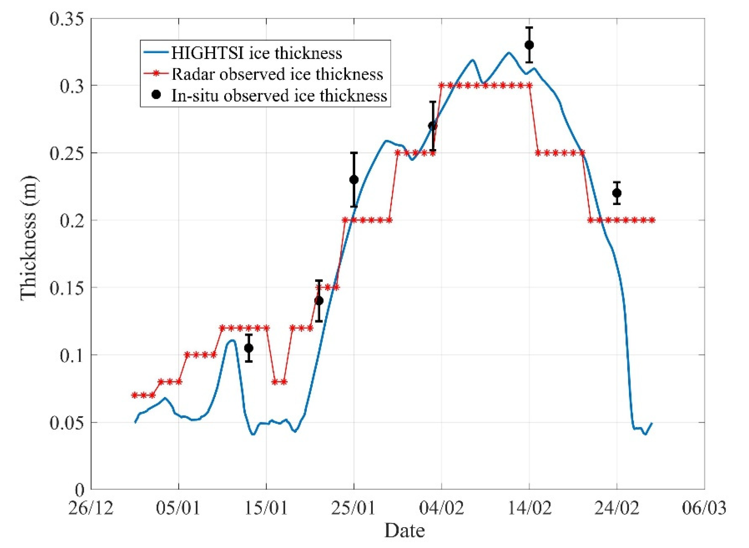
Bohai Sea in situ observations have been used for HIGHTSI development and validation [29]. This work was carried out more than 2 decades ago, and the validation period was rather short (~5–7 days). To perform multi-decadal seasonal modeling, a new validation of HIGHSTI for the Bohai Sea ice is necessary. The 2017/2018 seasonal-radar-observed ice thickness was selected for HIGHTSI validation. In addition, the monthly observed ice thickness was also applied as a seasonal ice survey. The BoSI was 3 for 2017/2018. The seasonal maximum level ice thickness reached 30 cm in Liaodong Bay. The maximum ice extent was reached on 28 January 2018, where the distance between the northernmost shoreline of Liaodong Bay and ice edge was approximately 137 km. The ice thickness was manually observed on the coastal landfast ice, and the situ observation was 4 km north of the Bayuquan coastal radar position. The level ice was 10 cm on 13 January 2018. On February 3, ice thickness reached 27 cm. On 14 February, ice thickness reached a seasonal maximum of 33 cm.
Figure 2 shows the comparison of observed and modeled ice thickness. We can see that HIGHTSI-modeled ice thickness captured the observed ice-growth pattern reasonably well during the freezing season (26 December–9 February). Bear in mind, this study focused on sea-ice thermodynamic modeling; the dynamic impact of sea ice was not considered in the HIGHTSI. Therefore, we cannot provide a quantitative assessment of wind and ocean impact on coastal ice accumulation. However, the local field observations indicated that offshore wind and ocean current can generate ice raft, leading to ice accumulation in the early freezing season [23]. The modeled maximum ice thickness was 0.32 m, whereas the in situ observed value was 0.33 m, so they were very close to each other. The modeled ice melting was faster than the observation. This discrepancy was probably contributed to by the ice dynamics. Melting reduces ice thickness, and thinner ice is easier to raft and deform, increasing the total ice thickness detected by the coastal radar and in situ point measurement. We concluded that HIGHTSI simulated seasonal landfast ice thickness near Yingkou until mid/late February.

Figure 2.
Seasonal evolution of modeled and observed ice thickness for 2017/2018 ice season. The vertical bar is the standard deviation of observed ice thickness.
3.2. Long-Term Trends of Meteorological Parameters
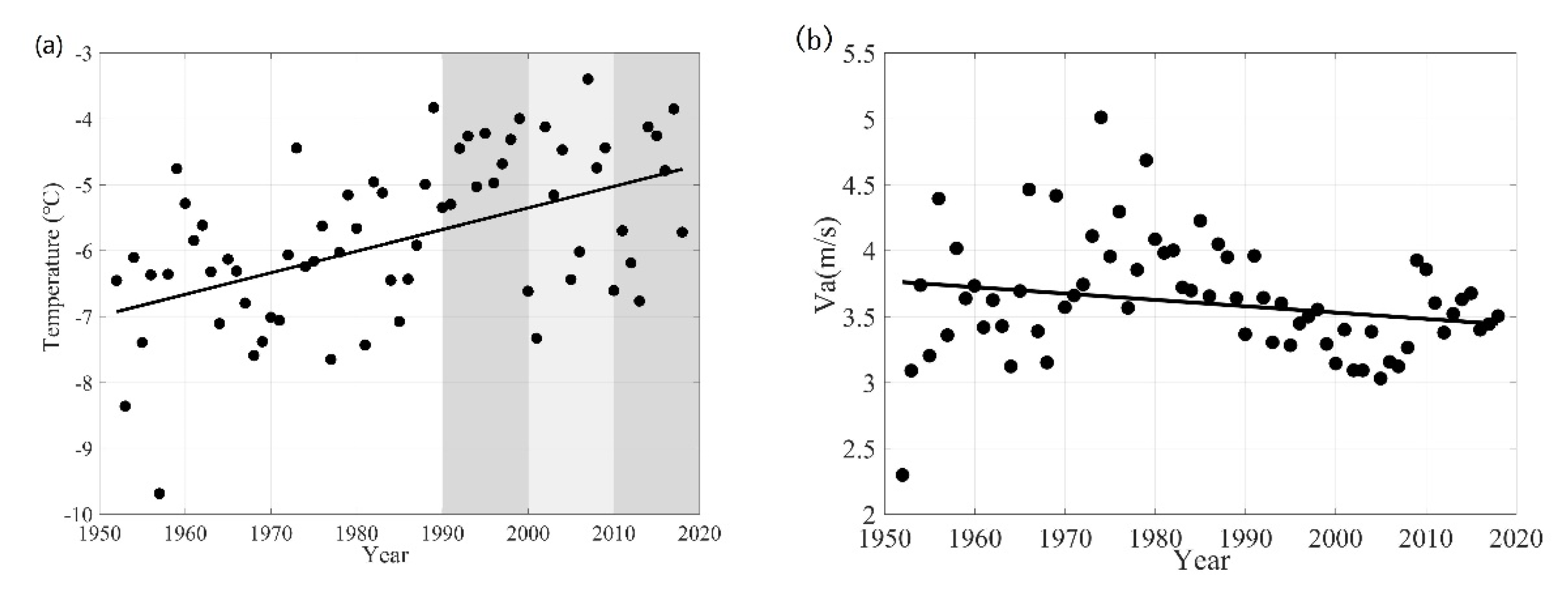
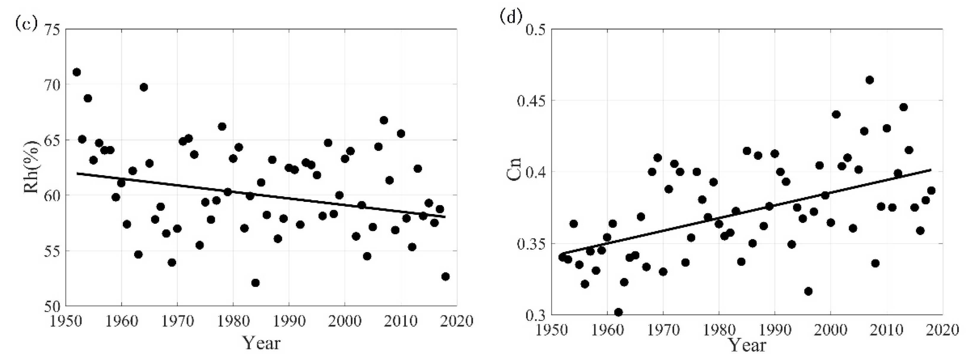
Figure 3 shows the observed winter-season mean meteorological parameters of Yingkou station during the study period. The air temperature shows an increasing trend of 0.33 °C/decade (Table 2). The wind speed has a decreasing trend of 0.05 m/s/decade. The relative humidity decreased by 0.59%/decade. Cloudy weather also increased.


Figure 3.
Multi-decadal (1950–2020) winter seasonal mean value of (a) air temperature, (b) wind speed, (c) relative humidity, and (d) total cloudiness. Each grey column marks one decade. The fitting lines were generated by using the Theil–Sen estimator.
Table 2.
Significance of trends (Mann–Kendall test) of meteorological parameters during the freezing season.
Table 3 summarized the average temperature trend for each winter month. The result indicated that increases in air temperature were the highest in February (the heaviest ice month for the Bohai Sea), followed by January (the second heaviest ice month) and December. The March air temperature increased the slowest during the Bohai Sea winter season. The increase in monthly mean temperature reached statistical significance during January and March. The increase in temperature has an important influence on the weakening of ice conditions.
Table 3.
Trends of air temperatures during the season of DJFM.
The increase in cloudy weather can reduce longwave radiative cooling, while cold weather generates local warming.
3.3. Sea-Ice-Mass Balance
3.3.1. Maximum Ice Thickness
HIGHTIS is a one-dimensional thermodynamic snow-and-ice model. The mass balance is simulated in the vertical direction. However, HIGHTSI can be used for 2D simulation for a domain if the weather data from each grid are provided [43]. In this study, we focused on the Yingkou coastal area. The calculated ice thickness refers to one unit area. The modeled ice thickness is representative for the coastal area, since the ice is immobile once consolidated. A total of 67 winters’ sea-ice thermodynamic mass balances were simulated (the computation is performed on the Qingdao National Laboratory for Marine Science and Technology high-performance computing and systematic simulation platform). The model run started on 1 December. The model was initialized with a constant 0.05 m thin ice. In early December, the weather conditions may not favor sea-ice formation; if the modeled ice thickness is smaller than 0.05 m, this value will be resumed. The initial ice freeze-up was defined as ice thickness starting to grow continuously [38]. The model run stopped when the ice thickness was reduced to zero. The initial 0.05 m ice thickness was justified because of the dynamic impact due to wave/tide and wind, meaning that the sea-ice thickness was rarely sustainable below 5 cm. Snow was not included in the simulations, since seasonal snow on sea ice was rather thin. The seasonal modeled maximum ice thickness versus BoSI is illustrated in Figure 4.

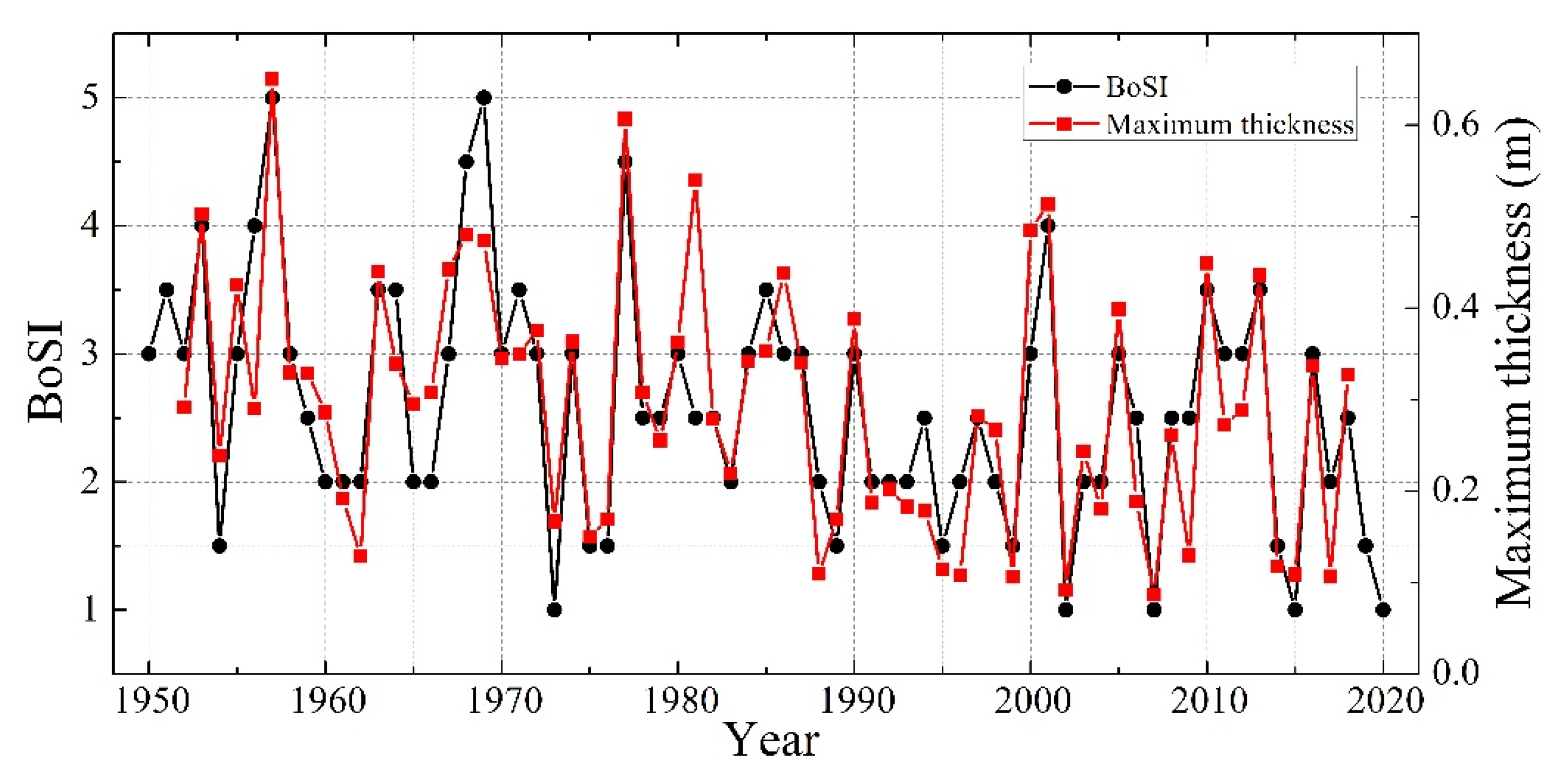
Figure 4.
HIGHTSI modeled seasonal maximum ice thickness (black squares) and the Bohai Sea ice index (BoSI).
The correlation coefficient between BoSI and modeled maximum ice thickness is 0.83 (p < 0.001) during the study period. BoSI is determined annually by the seasonal maximum ice extent, ice season duration, and maximum ice thickness observed in the entire Bohai Sea. The Yingkou coastal region has the longest ice season duration in the Bohai Sea. Once the landfast ice is consolidated, the ice cover likely remains until the melting season begins. Yingkou region usually has the longest ice season and thickest ice thickness in the Bohai Sea. Therefore, the modeled maximum ice thickness correlates quite well with BoSI.
3.3.2. Bohai Sea Ice Phenology
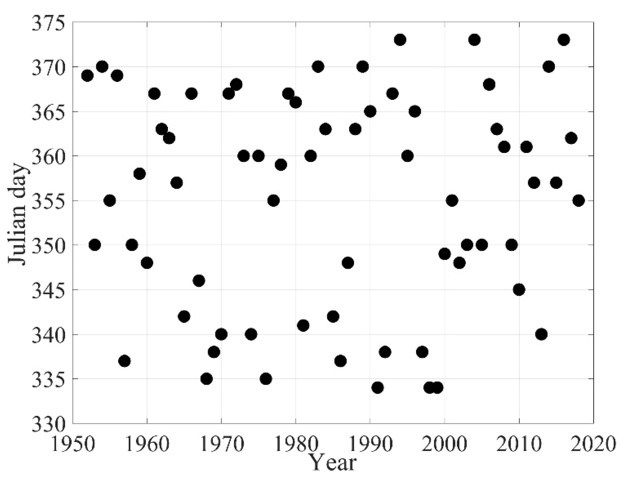
HIGHTSI modeled inter-annual freezing-up dates are shown in Figure 5. The earliest freezing-up occurred on 30 November, and the last was on 8 January. Previous studies have indicated that Bohai Sea ice conditions are largely dominated by the intensity and timing of cold-air outbreaks [44]. In December, under the influence of a cold swell and outbreaks from North Siberia, the low air temperature, accompanied with strong northwest wind, significantly cooled the seawater temperature in Liaodong Bay, leading to sea-ice formation. However, diurnal solar radiation was strong at Bohai Sea’s latitude. The clear sky weather prevails during winter. Hence, sea ice in the Liaodong Bay was often under the influence of repeated random frozen/thawed weather in early winter, leading to large interannual variations in the freezing-up date, without a long-term trend. On average, the freezing-up date occurred around 21 December.

Figure 5.
Modeled freezing-up date (black circles) for each winter season during study period.
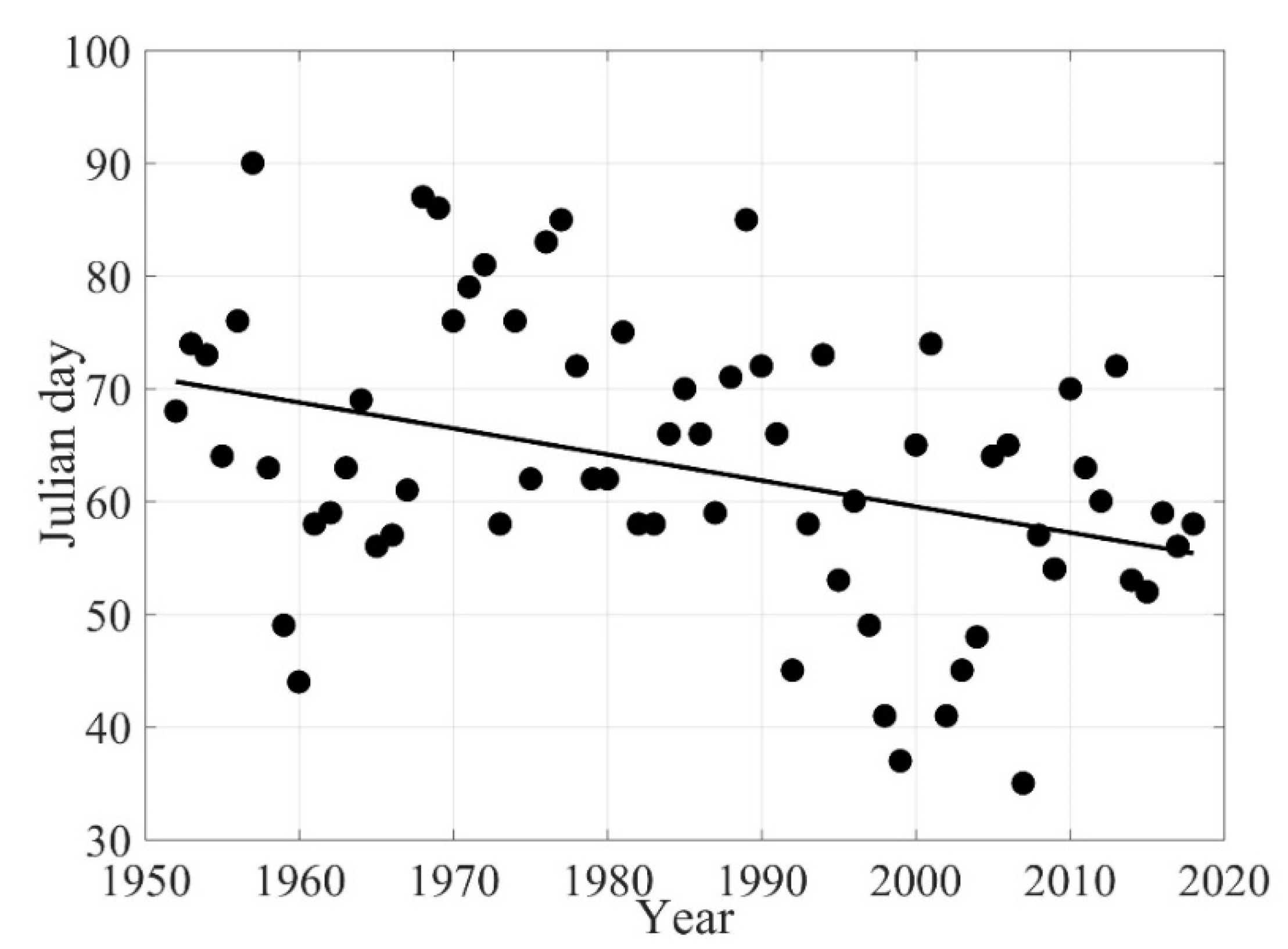
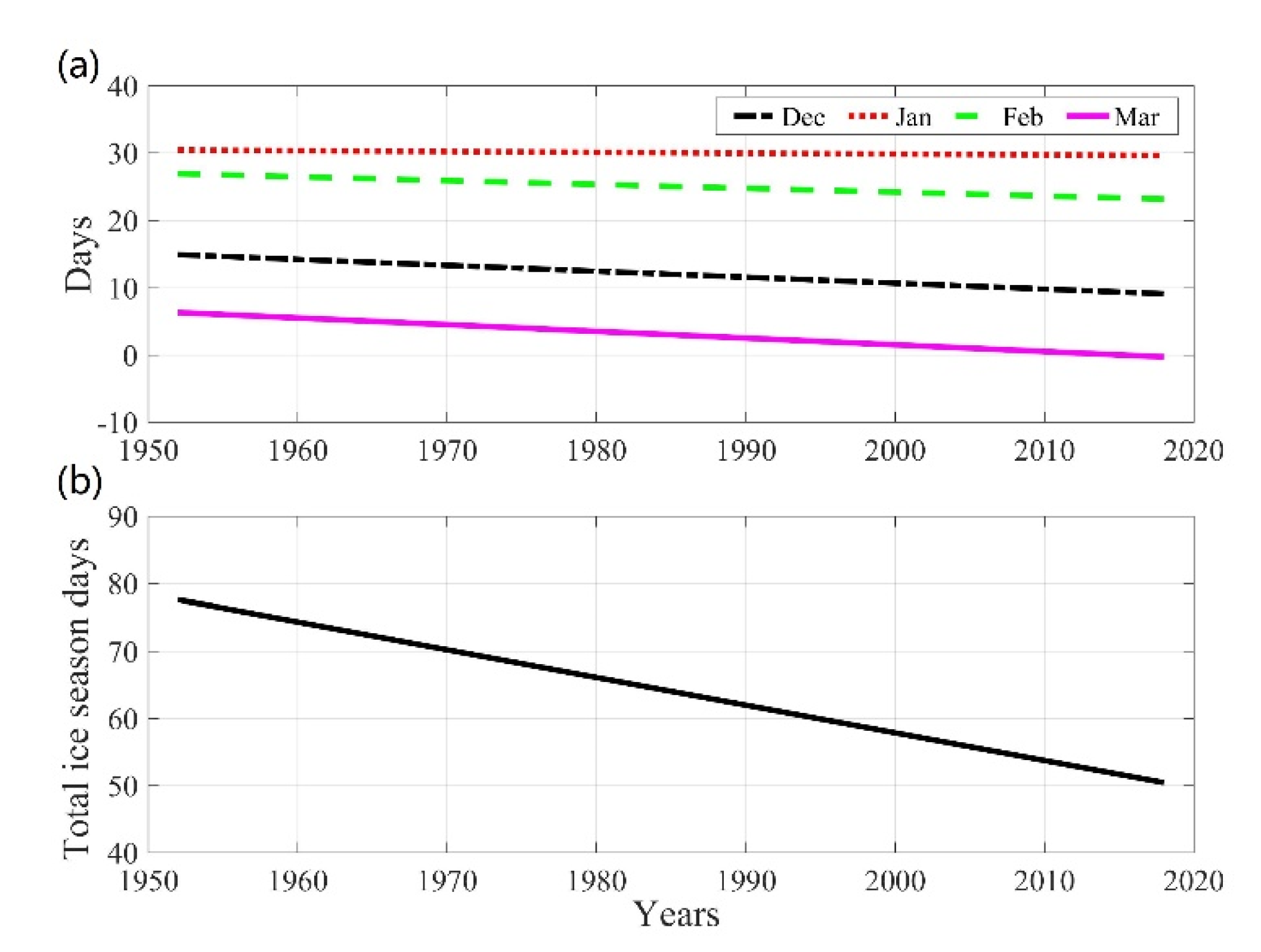
The modeled breakup date showed a clear trend toward early occurrence (Figure 6). The average breakup date was 4 March ± 12 (mean ± standard deviation), the earliest breakup date occurred on 5 February 2008, and the latest breakup date was 31 March 1958. The decreasing trend of the breakup date was 2.3 days/decade. The modeled breakup date was largely affected by the accumulated melting degree day, which is determined by air temperature above zero. The modeled accumulation of total number of ice-days (the number of days in which sea ice exists) in each month (Figure 7a) and for the entire ice season (FIS, Figure 7b) showed decreasing trends in response to the variability in freezing-up and breakup dates. The decreases in ice-days were large in March and December as compared with those in January and February. The average total number of ice-days was 69 ± 20. The decreasing trend of the ice season was 3.72 days/decade (Table 4).

Figure 6.
HIGHTSI modeled sea ice breakup date (black circles) for each winter season and fitting trend line generated by the Theil–Sen estimator.

Figure 7.
(a) Number of ice-days for each month. (b) Number of ice-days for entire winter season.
Table 4.
Trends of HIGHTSI-modeled seasonal ice-days and breakup date (Theil–Sen’s slope).
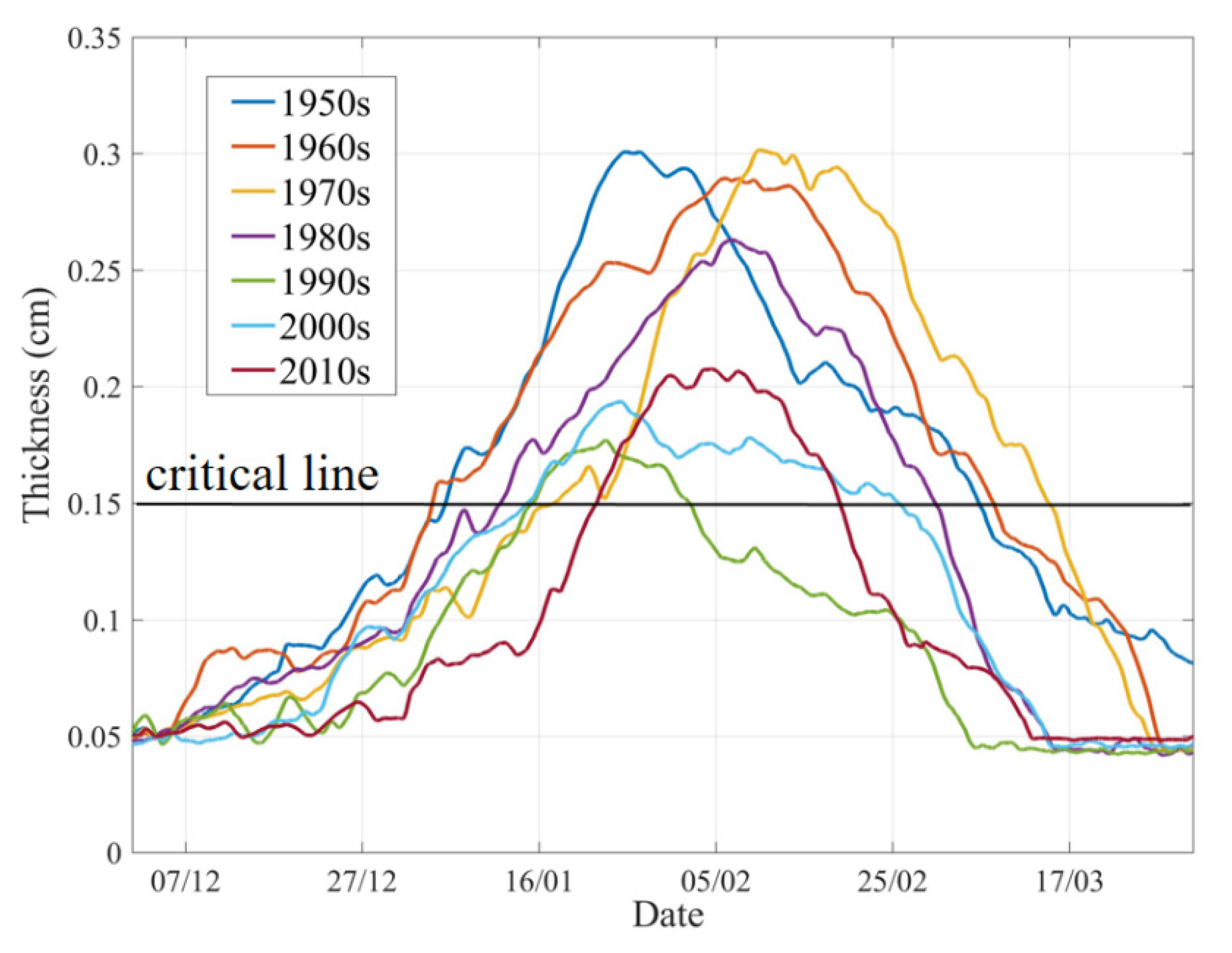
For Yingkou harbor, the operational sea-ice management authority defined 15 cm–level ice thickness as a critical condition for ships navigation in the region [45]. We can, therefore, divide seasonal ice evolution into three sessions: (i) a period from initial ice freeze-up until ice thickness reached 15 cm, (ii) a period where ice thickness is larger than 15 cm, and (iii) a period when ice thickness is below 15 cm until ice-free. Those sessions can be named the initial sea-ice stage (Ⅰ), heavy ice condition (Ⅱ), and melting period (Ⅲ). The heavy ice period has the greatest impact on economic activities. Based on these definitions, we calculated the timing of (Ⅰ) and (Ⅲ), and length of (Ⅱ) for each ice season and averaged each decade from the 1950s to 2010s. The numbers are summarized in Table 5, and the mean decadal ice evolution is plotted in Figure 8. Before the 1980s, the length of (Ⅱ) was longer and ice was thick; after the 1980s, the length of (Ⅱ) and ice thickness both decreased rapidly. The occurrence of (Ⅱ) is delayed from 3 January to 21 January, and the ending time of (Ⅱ) occurred early, from 6 March to 19 February.
Table 5.
Timing (onset and ending) and length of (Ⅱ) from the 1950s to the 2010s.

Figure 8.
Decadal average seasonal ice-thickness distribution and timing for different ice stages.
3.3.3. Sea-Ice Thickness
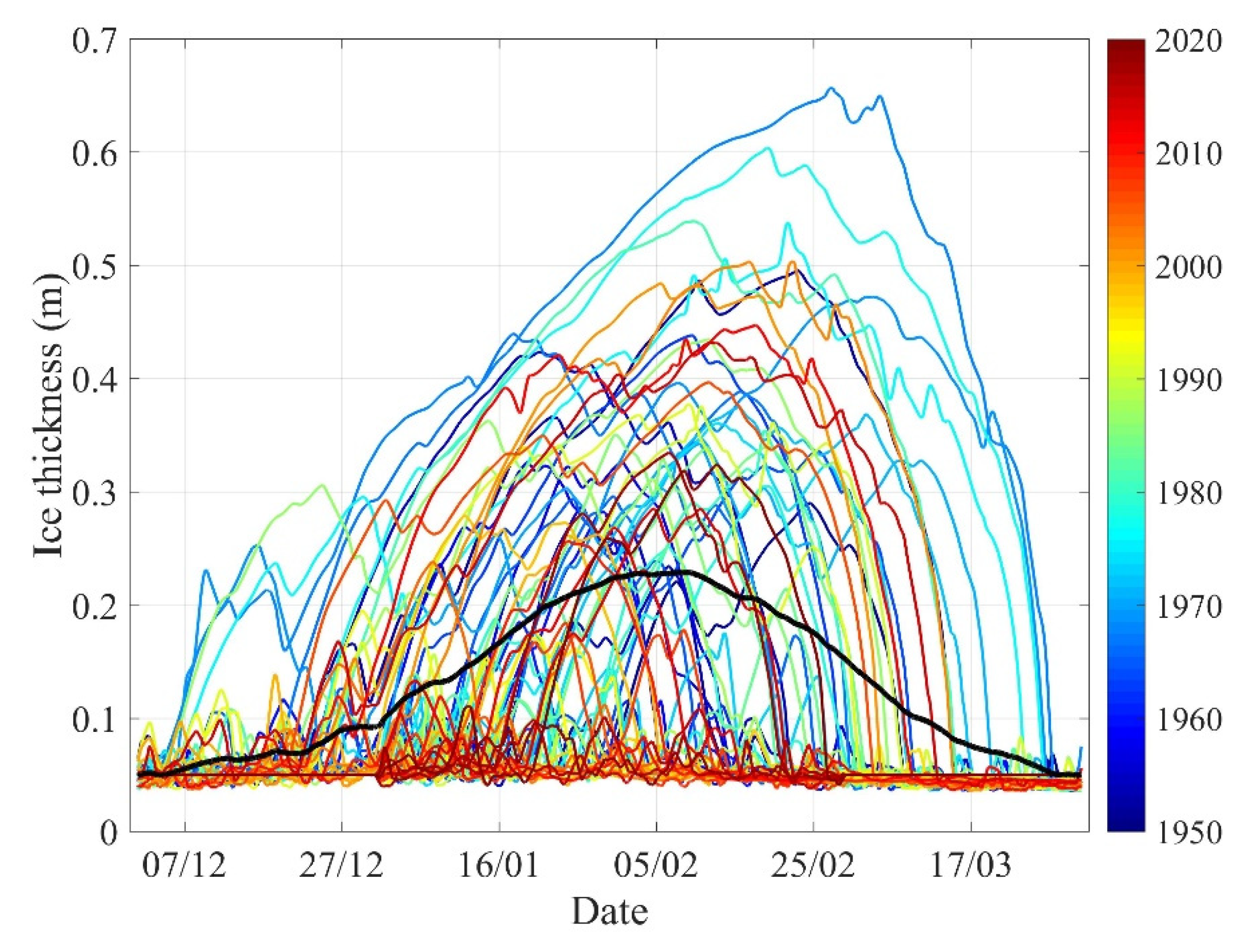
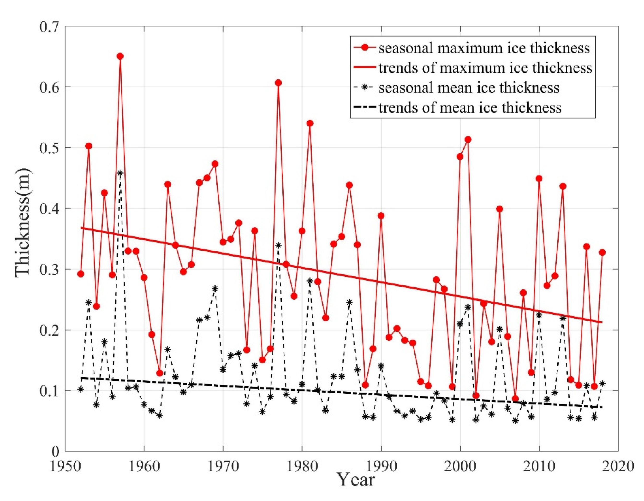
The seasonal evolution of modeled ice thicknesses for the 67 ice seasons and the average value are given in Figure 9. The seasonal ice-thickness evolution showed large interannual variations. The seasonal maximum ice thickness was 65 cm, as calculated on 27 February in 1956. The corresponding minimum value was 8.6 cm at early February in 2008. The multi-decadal mean ice thickness showed a quite symmetrical distribution with a multi-decadal maximum ice thickness of about 0.24 cm in the beginning of February. The modeled seasonal average and maximum ice thickness are given in Figure 10. Both maximum and mean ice thickness reveal decreasing trends of 2.55 and 0.76 cm/decade, respectively. The trends reached statistical significance (Table 6). The average date of the annual maximum ice thickness was February 4 ± 13 days.

Figure 9.
Seasonal evolution of modeled ice thicknesses for 67 ice seasons (1951/1952–2017/2018). The thick black line is the modeled seasonal average ice thicknesses. The color bar represents the ice season in the figure.

Figure 10.
Maximum and average ice thicknesses for the winter 1951/1952–2017/2018. The lines are trends of ice thicknesses (p < 0.05).
Table 6.
Trends of seasonal ice thicknesses.
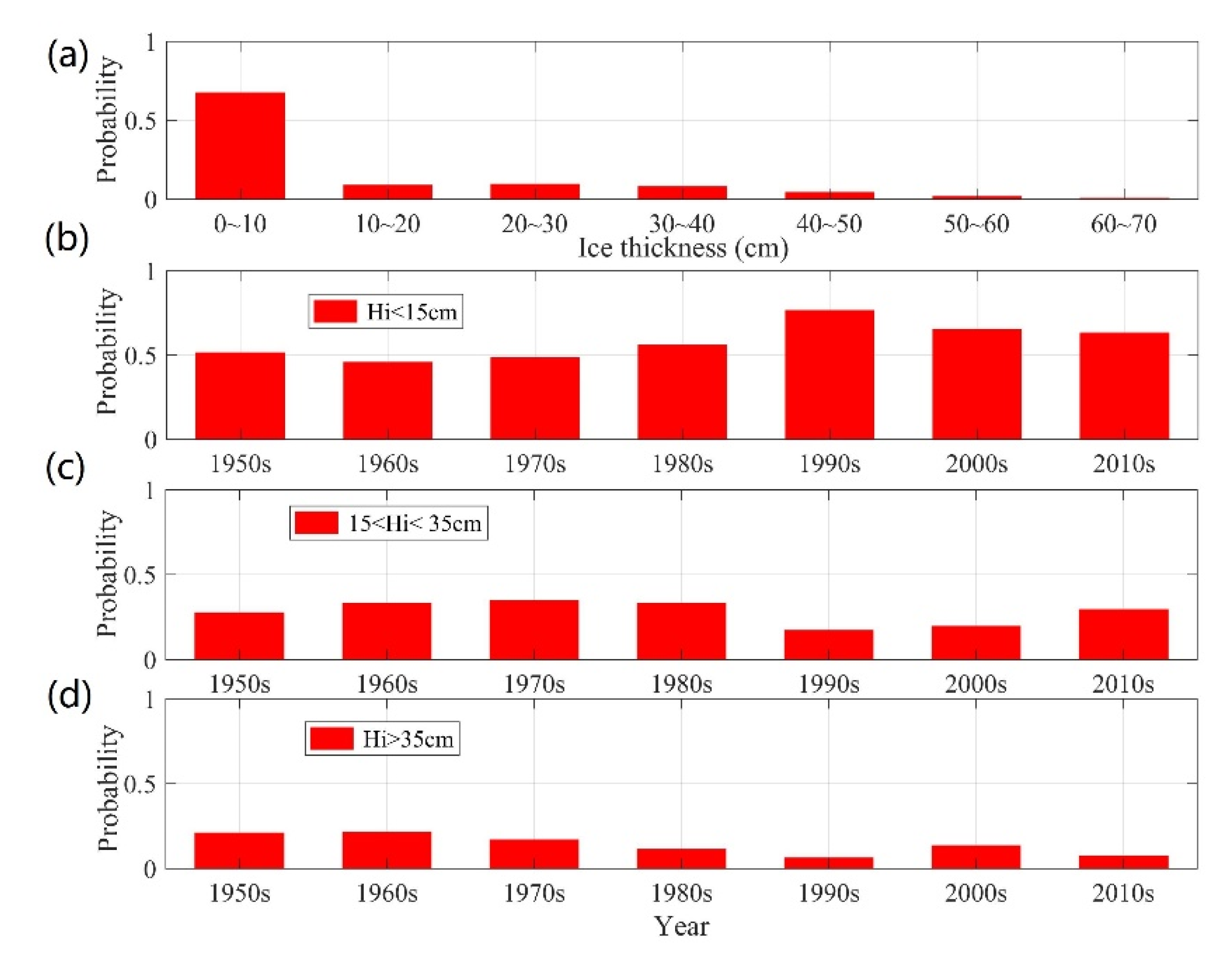
The quantitative ice thickness is a key parameter for offshore infrastructure design and maritime navigation safety management. Modeled ice thickness can be used for assessment. Figure 11a shows the probability density function (PDF) of modeled seasonal ice thickness distribution during the entire study period (1952/1952–2017/2018), using 10 cm bin. The ice thickness ranging between 0 and 10 cm has the highest probability (67%). For the ice-thickness groups of [10–20 cm], [20–30 cm], and [30–40 cm], the probabilities have the same magnitudes (8.0–9.5%). For ice thicknesses larger than 40 cm, the probability exponentially decreased.

Figure 11.
(a) Probability of ice thickness (grouped every 10 cm) distribution in the winter of 1951/1952–2017/2018. The probability of ice thickness in different thickness categories between 0 and 15 cm in (b), between 15 and 35 cm in (c) and larger than 35 cm in (d).
The PDFs of different ice-thickness categories, along with time, are illustrated in Figure 11b–d. For ice thickness less than 15 cm (Figure 11b), the 1990s has the highest PDF. For ice thickness between 15 and 35 cm (Figure 11c), the PDF was high in the 1970s, followed by the 1980s and 1960s. In the 2010s, this ice category was clearly more than that in the 1990s and 2000s. Ice thickness in the early 1990s has the largest thin-ice category. A better understanding of extreme ice-thickness conditions is important for sea-ice management to ensure the safety of winter navigation, offshore infrastructure, and harbor operations. Based on the definition of climate extremes indices (percentile definition method), we defined 90% percentile modeled ice thickness as a quantitative index for extreme ice conditions. This value read as 35 cm. The probability of an ice thickness greater than 35 cm for each decade is shown in Figure 11d. The probability of extreme ice thickness has a clear decreasing trend. The probability of occurrence of extreme ice thickness in the 1990s and 2010s is lower, by about 60%, than that in 1960s.
3.4. Large-Scale Atmospheric Circulation
Table 7 summarizes the correlations between the winter large-scale atmospheric indices and observed mean meteorological parameters between December and March from 1951/1952 to 2017/2018 and the BoSI index. AO and NAO were correlated in terms of BoSI, air temperatures, and average and maximum ice thicknesses, whereas the PNA, PDO, and ENSO had no statistically significant correlations. We can conclude AO and NAO have links with sea-ice conditions in the Yingkou area.
Table 7.
Correlation coefficients.
The interannual ice-condition changes in the Yingkou region are mainly influenced by the local and regional weather and climate patterns. The high pressure in the Siberian High Arctic is closely related to China’s winter climate. High pressure in the Siberian winter season may bring cold air southward. When the AO is positive, the Arctic region is controlled by low atmospheric pressure, the corresponding cold air will shrink in the vicinity of the Arctic, and the temperature of the mid-latitudes will be higher. When the AO moves negatively, the Arctic is controlled by high atmospheric pressure, and the cold air in the polar region is squeezed southward. In winter, when the AO is in a positive/negative anomaly, the Yingkou region ice condition tends toward being mild/severe. In the years when the NAO Index was strong, the intensity of the Azores high was likely weak, corresponding to the weak high pressure in Siberia. The impact of NAO on the ice condition in Yingkou is similar to that of AO [46,47].
4. Discussions
Long-term sea-ice process-modeling studies have been rare for the Bohai Sea, due to the limited in situ observations. However, long-term sea-ice-area analyses have been investigated before, using BoSI and remote-sensing observation [18]. Our results are in line with long-term variations in sea-ice area in the Bohai Sea. For example, Yan [18] found that the maximum and average Bohai Sea ice cover showed decreasing trends between 1958 and 2015, as also reflected by the decrease in the maximum and mean ice thickness calculated in this study. However, there are differences. For example, Yan [18] found that the Bohai Sea ice cover increased between 1958 and 1980, followed by a decreasing period between 1980 and 1995; then it increased again between 1995 and 2015, i.e., a weak periodical variation. Our modeled maximum and average ice thickness did not reveal such periodical variation during the simulation period. One possible explanation for this is that our result was confined to the Yongkou region based on a physical model, while Yan targeted the entire Bohai Sea, using statistical analyses. The modeled Yongkou ice thickness is not necessarily representative of the entire Bohai Sea. The statistical method may not be representative of the complicated physical world.
The HIGHTSI-modeled seasonal maximum ice thickness was correlated with BoSI. However, there was an exception. For the extreme Bohai Sea ice season of 1968/1969, where BoSI was the highest, HIGHTSI-modeled maximum ice thickness, however, was not the multi-decadal maximum value. The entire Bohai Sea was covered by sea ice in March 1968/1969, making it the severest ice winter in the last 70 years. The mismatch between modeled Yingkou maximum ice thickness and highest BoSI may be caused by the fact that the HIGHTSI result represents only the thermodynamic ice mass balance, while BoSI represents both the sea-ice thermodynamics (ice-season duration) and dynamics (maximum ice extent) of the entire Bohai Sea. There are many factors that impact the extent of the ice. The wind is the most important factor. In the winter, the Bohai Sea usually faces a northwest wind and north wind, meaning that Liaodong Bay has the most serious ice conditions in the Bohai Sea. In the winter of 1969, the Bohai Sea area prevailed with a northeast wind, which led to the Bohai Bay having the most serious ice conditions in the Bohai Sea. The HIGHTSI-modeled maximum ice thickness is comparable to the situation in the Liaodong Bay. The highest BoSI of 1968/1969 was attributed to severe ice conditions in another part of the Bohai Sea.
The trend in meteorological parameters, particularly the increasing air temperature in Yingkou, was comparable to the air temperature increase around the Bohai Sea [13]. The average air temperature increased by 0.27 °C per decade around the Bohai Sea. The temperature increase in Yingkou was slightly (0.06 °C) higher than that. However, far north (67N) in the boreal Nordic Arctic region, the increase in air temperature was much faster (1.03 °C per decade) [39], a good example of polar amplification [48]. In the mid-latitude monsoon climate zone, the warming rate was less than that in the Northern Polar region [49]. The decreasing wind speed trend (0.05 m/s per decade) in Yingkou was a lot weaker than that found by a study (0.3 m/s per decade) averaged around the entire Bohai Sea [50]. This is largely caused by the impact of investigation period. This large wind decreasing trend in Reference [50] was derived from the data observed between 1971 and 2012, where the wind speed was the highest in the 1970s and the lowest in the 2000s. The humidity trend found in Yingkou (0.6 per decade) was in line with the humidity trend (0.8 per decade) in Northeast China between 1951 and 2000 [51].
Our results indicated that mean and maximum ice thickness in Yingkou are correlated with AO and NAO, with statistical significance. This result agreed with a previous study stating that the severity of the entire Bohai Sea ice was correlated with AO [22]. Gong et al. 2007 [22] found that the Bohai Sea ice severity has declined rapidly since the 1970s. This was in line with our results, showing that the probability of thinner ice (<15 cm) increased drastically between the 1970s and 1990s (Figure 11b), although ice thickness showed some increases in the 2000s and 2010s. Nevertheless, the trends in our modeled ice parameters are reasonably consistent with long-term regional investigations [13,17,18].
The modeled ice freezing-up date remains a challenge for coastal regions [38,52,53]. The Bohai Sea is a semi-enclosed sea; the seawater salinity was lower than that in the open ocean. The coastal shadow water may be mixed in early winter before the ice season starts. The sea-ice formation results from the heat loss from seawater to the atmosphere. However, due to the tides, sea wave, and random inter-exchanges of cold swells and thaw in early winter, the initially frozen sea ice is likely to break off and refreeze again. When the ice is thin, due to the impact of tide and wind, the ice cover may break up, raft, or even creep up to the beach. A wave/tide–ice coupled model would be needed to better understand this dynamic process. Once the coastal sea ice is consolidated, the ice-mass balance is dominated by the thermodynamic processes. Further away from the coastal area, the dynamic ice formation may prevail [43]. During the melting period, the ice thickness grows thinner. The ice floes are, again, more easily subject to the effect of tide, wave, and wind. The ice floes may be more dynamic and could result in thicker ice, as compared with the thermodynamic modeled ice thickness. This process was not considered in the HIGHTSI model.
Another simplification in this study is the neglection snow. Differing from other seasonal ice-covered seas, e.g., the Baltic Sea, where snow can be as high as 20–30 cm seasonally [19], the snow on the Bohai Sea ice is indeed very thin and can be neglected [54]. However, climate warming may lead to more snowfall in the future [55], even in the Bohai Sea. Therefore, we would need high-quality precipitation observation, which is vitally important for snow modeling.
5. Conclusions
Multi-decadal sea-ice thickness in Yingkou, a coastal region located northeast of the Bohai Sea, was simulated by an ice thermodynamic process model (HIGHTSI). A total of 67 ice seasons were simulated by using local weather station data as external forcing. The ice phenology, mass balance, and their interannual trends were investigated. To the best of our knowledge, this study is the longest interannual ice-mass-balance simulation ever carried out for the Bohai Sea. The seasonal ice-mass balance in the Yingkou region was modeled quite well by HIGHTSI. For the model validation experiment, HIGHTSI-modeled ice growth, the maximum ice thickness, and timing of onset melting were close to the in situ observations and coastal-radar-retrieved ice thickness. The mean observed and modeled ice growth rates were 1.57 and 1.62 cm/day, respectively, which were quite close to each other. The difference between the calculated and observed maximum ice thickness was very small (1 cm).
The multi-decadal ice phenology indicated a decrease in maximum ice thickness, shortened ice season, and early breakup date. Those results are comparable with previous studies by Gong [17] and Yan [18], where the regional Bohai Sea ice was investigated. In addition, the simulated ice thickness in the YingKou area was getting thinner continuously since 1951/1952. There was a significant weakening of ice conditions in the 1990s in response to the warm weather.
The collection of on-site observation data is very important. Ice radar-data analysis can help us understand the evolution of sea ice. A combined ice radar and numerical model methodology can help us better understand the local ice breakup process. For the fracture process of sea ice in the sea near Yingkou, with the increase in solar radiation, the increase in water temperature at the ice bottom, and the decrease in sea ice cover area, sea ice rapidly decomposes under the combined action of thermal factors and dynamic factors. Our results indicated that the increase in solar radiation in late February has a controlling effect on the melting of sea ice. Bohai Sea ice melts rapidly during this period [28].
The ice condition has an important impact on the economic activities in Liaodong Bay. This study shows that the seasonal maximum ice thickness, length of ice season, and timing of breakup date are important parameters to evaluate the sea-ice severity. Taking the offshore oil platform as an example, we see that the magnitude of static ice force and dynamic ice force is determined by the maximum ice thickness and average ice thickness, respectively. The impact of ice load on an offshore structure is determined by the length of the sea season. The ice condition may also be affected by the regional environmental factors; for example, the inflow of river water may contain substances that will affect the sea water salinity and induce the biochemical processes which may affect the ice-formation and -melting processes. To understand those processes, we need sustainable in situ biochemical processes’ observations. The accurate assessment of ice conditions is crucial for sea-ice management and disaster prevention and mitigation in marine economic activities. HIGHTSI-modeled seasonal maximum ice thickness can be used as a proxy to assess the Bohai Sea ice climate in the future. One possibility would be to run HIGHTSI, applying results from the next generation of climate model CIMP6 future climate scenarios. The modeled ice parameters can be linked with the future BoSI.
Author Contributions
N.X. and S.Y. initiated this work; Y.M. and B.C. carried out modeling experiments, analyzed the results and wrote the original draft; H.S. and W.S. collected the data. All the authors contributed to the writing and editing of the manuscript. All authors have read and agreed to the published version of the manuscript.
Funding
Y.M., N.X., H.S., W.S. and S.Y. were financially supported by The National Key Research and Development Program of China (Grant No. 2017YFA0604901), National Natural Science Foundation of China (Grant No. U1806214) and Science and Technology Talents Program of Dalian (Grant No. 2019RJ07); B.C. was financially supported by Academy of Finland (Grant No. 317999).
Institutional Review Board Statement
Not applicable.
Informed Consent Statement
Not applicable.
Data Availability Statement
Meteorological data (http://data.cma.cn/, accessed on 1 December 2021); data of the sea ice index (http://www.soa.gov.cn/zwgk/hygb/zghyzhgb/, accessed on 1 December 2021 and Compilation of information on 40 years of marine disasters in China (1949–1990)); large-scale atmospheric circulation indices (www.esrl.noaa.gov/psd/data/climateindices, accessed on 1 December 2021).
Conflicts of Interest
The authors declare no conflict of interest.
References
- Rind, D.; Healy, R.; Parkinson, C.; Martinson, D. The role of sea ice in 2 × CO2 climate model sensitivity: Part I. The total influence of sea ice thickness and extent. J. Clim. 1995, 8, 449–463. [Google Scholar] [CrossRef] [Green Version]
- Holland, M.M.; Bitz, C.M. Polar amplification of climate change in coupled models. Clim. Dyn. 2003, 21, 221–232. [Google Scholar] [CrossRef]
- Nichols, T.; Berkes, F.; Jolly, D.; Snow, N.B. Community of Sachs Harbour. Climate change and sea ice: Local observations from the Canadian Western Arctic. Arctic 2004, 57, 68–79. [Google Scholar] [CrossRef] [Green Version]
- Wang, Y.; Yue, Q.; Bi, X. Field test system for investigating dynamic ice forces on jacket structures and platform safety guarantee in the Bohai Sea. Ocean. Eng. 2014, 78, 52–61. [Google Scholar] [CrossRef]
- Zhang, Y.; Jin, B.; Feng, X. Response of the Sea Ice Conditions in the Bohai Sea to the Global Climate Change in the Last Over Half Century. Mar. Sci. Bull. Tianjin Chin. Ed. 2007, 26, 96. [Google Scholar]
- Wu, H.D. Bohai sea ice design and operation conditions. China Ocean. Press Beijing 2001, 27–36. (In Chinese) [Google Scholar]
- Vihma, T.; Haapala, J. Geophysics of sea ice in the Baltic Sea: A review. Prog. Oceanogr. 2009, 80, 129–148. [Google Scholar] [CrossRef]
- Gu, W. Research on the sea-ice disaster risk in Bohai Sea based on the remote sensing. J. Catastrophol. 2008, 23, 10–14. [Google Scholar]
- Yuan, S.; Liu, C.; Liu, X.; Chen, Y.; Zhang, Y. Research advances in remote sensing monitoring of sea ice in the Bohai sea. Earth Sci. Inform. 2021, 4, 1729–1743. [Google Scholar] [CrossRef]
- Liu, C.; Chao, J.; Gu, W.; Xu, Y.; Xie, F. Estimation of sea ice thickness in the Bohai Sea using a combination of VIS/NIR and SAR images. GIScience Remote Sens. 2015, 52, 115–130. [Google Scholar] [CrossRef]
- Su, H.; Wang, Y.; Yang, J. Monitoring the spatiotemporal evolution of sea ice in the Bohai Sea in the 2009–2010 winter combining MODIS and meteorological data. Estuaries Coasts 2012, 35, 281–291. [Google Scholar] [CrossRef] [Green Version]
- Zhang, N.; Wu, Y.; Zhang, Q. Detection of sea ice in sediment laden water using MODIS in the Bohai Sea: A CART decision tree method. Int. J. Remote Sens. 2015, 36, 1661–1674. [Google Scholar] [CrossRef]
- Ouyang, L.; Hui, F.; Zhu, L.; Cheng, X.; Cheng, B.; Shokr, M.; Zhao, J.; Ding, M.; Zeng, T. The spatiotemporal patterns of sea ice in the Bohai Sea during the winter seasons of 2000–2016. International Journal of Digital Earth 2017, 12, 893–909. [Google Scholar] [CrossRef]
- Yuan, S.; Liu, C.; Liu, X. Practical model of sea ice thickness of Bohai Sea based on MODIS data. Chin. Geogr. Sci. 2018, 28, 863–872. [Google Scholar] [CrossRef] [Green Version]
- Yuan, S.; Gu, W.; Liu, C.; Xie, F. Towards a semi-empirical model of the sea ice thickness based on hyperspectral remote sensing in the Bohai Sea. Acta Oceanol. Sin. 2017, 36, 80–89. [Google Scholar] [CrossRef]
- Li, N.; Gu, W.; Maki, T.; Hayakawa, S. Relationship between sea ice thickness and temperature in Bohai Sea of China. J. Fac. Agric. Kyushu Univ. 2005, 50, 165–173. [Google Scholar] [CrossRef]
- Gong, D.Y.; Kim, S.J.; Ho, C.H. Arctic Oscillation and ice severity in the Bohai Sea, East Asia. Int. J. Climatol. J. R. Meteorol. Soc. 2007, 27, 1287–1302. [Google Scholar] [CrossRef]
- Yan, Y.; Uotila, P.; Huang, K.; Gu, W. Variability of sea ice area in the Bohai Sea from 1958 to 2015. Sci. Total Environ. 2020, 709, 136164. [Google Scholar] [CrossRef]
- Mäkynen, M.; Karvonen, J.; Cheng, B.; Hiltunen, M.; Eriksson, P. Operational Service for Mapping the Baltic Sea Landfast Ice Properties. Remote Sens. 2020, 12, 4032. [Google Scholar] [CrossRef]
- Karvonen, J.; Cheng, B.; Vihma, T.; Arkett, M.; Carrieres, T. A method for sea ice thickness and concentration analysis based on SAR data and a thermodynamic model. Cryosphere 2012, 6, 1507–1526. [Google Scholar] [CrossRef] [Green Version]
- Yang, G. Bohai Sea ice conditions. J. Cold Reg. Eng. 2000, 14, 54–67. [Google Scholar] [CrossRef]
- Li, Z.J.; Kang, J.C.; Pan, Y.B. Characteristics of the Bohai Sea and Arctic sea ice fabrics and crystals. Acta Oceanol. Sin. 2003, 25, 48–53. [Google Scholar]
- Bai, S.; Liu, Q.Z.; Li, H.; Wu, H.D. Sea ice in the Bohai sea of China. Mar. Forecast. 1999, 3, 45–52. [Google Scholar]
- Wang, J.X.; Zhao, Z.J.; Shang, K.Z.; Wang, J.; Lei, G.G. Spatial and temporal distribution of cloud covers in the Bohai Sea region. J. Lanzhou Univ. Nat. Sci. 2019, 55, 125–130, 140. [Google Scholar]
- Dong, X. China’s first shore-based ice radar station has been built. J. Glaciol. Geocryol. 1989, 11, 260. (In Chinese) [Google Scholar]
- Ma, Y.; Guan, P.; Xu, N.; Xu, Y.; Yuan, S.; Liu, Y.; Xu, F. Determination of the sea ice parameters for the reliability design of the marine structures in Liaodong Bay. Ocean. Eng. 2019, 3, 136–142. (In Chinese) [Google Scholar]
- Yuan, S.; Shi, W.Q.; Liu, X.; Xu, N.; Chen, W. Erratum to: Ice type extraction of rough ice in the eastern coast of Liaodong bay with shore-based radar. Nat. Hazards 2015, 76, 1263–1273. [Google Scholar] [CrossRef]
- Yuan, S.; Liu, Y.Q.; Liu, X.Q. Basic characteristics of sea ice in the Bayuquan region based on the data of shore-based radar. Mar. Sci. Bull. 2017, 36, 528–531. (In Chinese) [Google Scholar]
- Launiainen, J.; Cheng, B. Modelling of ice thermodynamics in natural water bodies. Cold Reg. Sci. Technol. 1998, 27, 153–178. [Google Scholar] [CrossRef]
- Cheng, B.; Vihma, T.; Launiainen, J. Modelling of the superimposed ice formation and sub-surface melting in the Baltic Sea. Geophysica 2003, 39, 31–50. [Google Scholar]
- Cheng, B.; Vihma, T.; Pirazzini, R.; Granskog, M.A. Modelling of superimposed ice formation during the spring snowmelt period in the Baltic Sea. Ann. Glaciol. 2006, 44, 139–146. [Google Scholar] [CrossRef] [Green Version]
- Cheng, B.; Zhang, Z.; Vihma, T.; Johansson, M.; Bian, L.; Li, Z.; Wu, H. Model experiments on snow and ice thermodynamics in the Arctic Ocean with CHINARE 2003 data. J. Geophys. Res. 2008, 113, C09020. [Google Scholar] [CrossRef] [Green Version]
- Yang, Y.; Leppäranta, M.; Cheng, B.; Li, Z. Numerical modelling of snow and ice thicknesses in Lake Vanajavesi, Finland. Tellus A Dyn. Meteorol. Oceanogr. 2012, 64, 17202. [Google Scholar] [CrossRef] [Green Version]
- Cheng, B.; Vihma, T.; Rontu, L.; Kontu, A.; Pour, H.K.; Duguay, C.; Pulliainen, J. Evolution of snow and ice temperature, thickness and energy balance in Lake Orajärvi, northern Finland. Tellus A Dyn. Meteorol. Oceanogr. 2014, 66, 21564. [Google Scholar] [CrossRef]
- Maykut, G.A.; Untersteiner, N. Some results from a time-dependent thermodynamic model of sea ice. J. Geophys. Res. 1971, 76, 1550–1575. [Google Scholar] [CrossRef]
- Zhao, J.C.; Cheng, B.; Vihma, T.; Heil, P.; Hui, F.; Shu, Q.; Zhang, L.; Yang, Q. Fast ice prediction system (fips) for land-fast sea ice at prydz bay, east antarctica: An operational service for chinare. Ann. Glaciol. 2020, 61, 271–283. [Google Scholar] [CrossRef]
- Cheng, B.; Vihma, T.; Palo, T.; Palo, T.; Nicolaus, M.; Gerland, S.; Rontu, L.; Haapala, J.; Perovich, D. Observation and modelling of snow and sea ice mass balance and its sensitivity to atmospheric forcing during spring and summer 2007 in the Central Arctic. Adv. Pol. Sci. 2021, 32, 309–323. [Google Scholar]
- Zhai, M.; Cheng, B.; Leppäranta, M.; Hui, F.; Li, X.; Demchev, D.; Lei, R.; Cheng, X. The seasonal cycle and break-up of Landfast Sea ice along the northwest coast of Kotelny Island, East Siberian Sea. J. Glaciol. 2021, 1–13. [Google Scholar] [CrossRef]
- Mallick, J.; Talukdar, S.; Alsubih, M.; Salam, R.; Ahmed, M.; Kahla, N.B.; Shamimuzzaman, M. Analyzing the trend of rainfall in Air region of Saudi Arabia using the family of Mann-Kendall tests, innovative trend analysis, and distended fluctuation analysis. Theor. Appl. Climatol. 2021, 143, 823–841. [Google Scholar] [CrossRef]
- Kumar, K.S.; Rathnam, E.V. Analysis and prediction of groundwater level trends using four variations of Mann Kendall tests and ARIMA modelling. J. Geol. Soc. India 2019, 94, 281–289. [Google Scholar] [CrossRef]
- Ashraf, M.S.; Ahmad, I.; Khan, N.M.; Zhang, F.; Bilal, A.; Guo, J. Stream flow Variations in Monthly, Seasonal, Annual and Extreme Values Using Mann-Kendall, Spearmen’s Rho and Innovative Trend Analysis. Water Resour. Manag. 2021, 35, 243–261. [Google Scholar] [CrossRef]
- Wei, L.; Deng, X.; Cheng, B.; Vihma, T.; Hannula, H.-R.; Qin, T.; Pulliainen, J. The impact of meteorological conditions on snow and ice thickness in an Arctic lake. Tellus A Dyn. Meteorol. Oceanogr. 2016, 68, 31590. [Google Scholar] [CrossRef] [Green Version]
- Karvonen, J.; Shi, L.; Cheng, B.; Similä, M.; Mäkynen, M.; Vihma, T. Bohai sea ice parameter estimation based on thermodynamic ice model and earth observation data. Remote Sens. 2017, 9, 234. [Google Scholar] [CrossRef] [Green Version]
- Zhang, N.; Wu, Y.; Zhang, Q. Forecasting the evolution of the sea ice in the Liaodong Bay using meteorological data. Cold Reg. Sci. Technol. 2016, 125, 21–30. [Google Scholar] [CrossRef]
- Zhang, F. Sea ice in China. Navig. China 1982, 2, 66–75. (In Chinese) [Google Scholar]
- Bai, X.; Wang, J.; Liu, Q.Z.; Wang, D.; Liu, Y. Severe ice conditions in the Bohai Sea, China, and mild ice conditions in the great lakes during the 2009/10 winter: Links to El Nino and a strong negative arctic oscillation. J. Appl. Meteorol. Clim. 2011, 50, 1922–1935. [Google Scholar] [CrossRef]
- Yan, Y.; Shao, D.D.; Gu, W.; Liu, C.; Li, Q.; Chao, J.; Tao, J.; Xu, Y. Multidecadal anomalies of Bohai Sea ice cover and potential climate driving factors during 1988–2015. Environ. Res. Lett. 2017, 12, 094014. [Google Scholar] [CrossRef]
- Overland, J.E.; Dethloff, K.; Francis, J.A.; Hall, R.J.; Hanna, E.; Kim, S.-J.; Screen, J.A.; Shepherd, T.G.; Vihma, T. Nonlinear response of mid-latitude weather to the changing arctic. Nat. Clim. Chang. 2016, 6, 992–999. [Google Scholar] [CrossRef] [Green Version]
- Yamanouchi, T. Early 20th century warming in the arctic: A review. Pol. Sci. 2011, 5, 53–71. [Google Scholar] [CrossRef] [Green Version]
- Guo, J.; Cao, J.F.; Yang, Y.J.; Tianjin, C.C. Variation of wind speed and its influencing factors around the Bohai coastal areas from 1971 to 2012. J. Meteorol. Environ. 2015, 31, 82–88. (In Chinese) [Google Scholar] [CrossRef]
- Wang, Z.Y.; Ding, Y.H.; He, J.H.; Jun, Y. An updating analysis of the climate change in china in recent 50 years. Acta Meteorol. Sin. 2004, 2, 228–236. [Google Scholar]
- Johansson, A.M.; Malnes, E.; Gerland, S.; Cristea, A.; Doulgeris, A.P.; Divine, D.V.; Pavlova, O.; Lauknes, T.R. Consistent ice and open water classification combining historical synthetic aperture radar satellite images from ERS-1/2, Envisat ASAR, RADARSAT-2 and Sentinel-1A/B. Ann. Glaciol. 2020, 61, 40–50. [Google Scholar] [CrossRef] [Green Version]
- Muckenhuber, S.; Nilsen, F.; Korosov, A.; Sandven, S. Sea ice cover in Isfjorden and Hornsund, Svalbard (2000–2014) from remote sensing data. Cryosphere 2016, 10, 149–158. [Google Scholar] [CrossRef] [Green Version]
- Liu, C.; Gu, W.; Chao, J.; Li, L.; Yuan, S.; Xu, Y. Spatio-temporal characteristics of the sea-ice volume of the Bohai Sea, China, in winter 2009/10. Ann. Glaciol. 2013, 54, 97–104. [Google Scholar] [CrossRef] [Green Version]
- Wang, C.; Cheng, B.; Wang, K.; Gerland, S.; Pavlova, O. Modelling snow ice and superimposed ice formation in an Arctic fjord. Polar Res. 2015, 34, 20828. [Google Scholar] [CrossRef] [Green Version]
Publisher’s Note: MDPI stays neutral with regard to jurisdictional claims in published maps and institutional affiliations. |
© 2022 by the authors. Licensee MDPI, Basel, Switzerland. This article is an open access article distributed under the terms and conditions of the Creative Commons Attribution (CC BY) license (https://creativecommons.org/licenses/by/4.0/).