Abstract
Suaeda salsa (L.) Pall. (S. salsa) acts as a pioneer species in coastal wetlands due to its high salt tolerance. It has significant biodiversity maintenance, socioeconomic values (e.g., tourism) due to its vibrant color, and carbon sequestration (blue carbon). Bohai Bay region, the mainly distributed area of S. salsa, is an economic intensive region with the largest economic aggregate and population in northern China. The coastal wetland is one of the most vulnerable ecosystems with the urbanization and economic developments. S. salsa in Bohai Bay has been changed significantly due to several threats to its habitat in past decades. In this paper, we analyzed all available archived Landsat TM/ETM+/OLI images of the Bohai Bay region by using a decision tree algorithm method based on the Google Earth Engine (GEE) platform to generate annual maps of S. salsa from 1990 to 2020 at a 30-m spatial resolution. The temporal-spatial dynamic changes in S. salsa were studied by landscape metric analysis. The influencing factors of S. salsa changes were analyzed based on principal component analysis (PCA) and a logistic regression model (LRM). The results showed that S. salsa was mainly distributed in three regions: the Liao River Delta (Liaoning Province), Yellow River Delta (Shandong Province), and Hai River Estuary (Hebei Province, Tianjin). During the past 31 years, the total area of S. salsa has dramatically decreased from 692.93 km2 to 51.04 km2, which means that 92.63% of the area of S. salsa in the Bohai Bay region was lost. In the 641.89 km2 area of S. salsa that was lost, 348.80 km2 of this area was converted to other anthropic land use categories, while 293.09 km2 was degraded to bare land. The landscape fragmentation of S. salsa has gradually intensified since 1990. National Nature Reserves have played an important role in the restoration of suitable S. salsa habitats. The analysis results for the natural influencing factors indicated that precipitation, temperature, elevation, and distance to the coastline were considered to be the major influencing factors for S. salsa changes. The results are valuable for monitoring the dynamic changes of S. salsa and can be used as effective factors for the restoration of S. salsa in coastal wetlands.
1. Introduction
Wetlands are often recognized as nature-based solutions that can provide a variety of comprehensive services that are of social, economic, and environmental value to humans [1]. Coastal wetlands are located where ocean and land are interspersed, and they are sensitive to external stresses and are vulnerable to human activities [2]. Coastal populations and wetlands have been intertwined for centuries and have experienced intense and varied human impacts [3]. Coastal wetlands, which mostly include tidal flats and coastal vegetation (e.g., mangroves and saltmarshes), are seriously threatened and have continuously decreased in their areas [4]. Many studies have been carried out on the restoration [5], evaluation, management, evolution mechanisms [6], biomass, and carbon storage in coastal wetlands [7]. However, more notably, vegetation, as an important component of coastal wetlands, can comprehensively reflect the characteristics of coastal wetlands. Vegetation changes can provide good indicators for understanding and evaluating the status of coastal wetlands. Some studies have found that the global vegetation densities in wetlands are decreasing due to climate change and the impacts of interference from human activities [8].
As an important salt-tolerant plant in coastal wetlands, S. salsa is an annual herbaceous euhalophyte with strong ecological tolerance and is an indicator plant with strong adaptability [9]. This species plays a key role in carbon sequestration (“blue carbon”), shoreline protection, pollutant reduction, and biodiversity maintenance [10]. In historical periods, excessive human activities (e.g., reclamation and aquaculture) and natural factors (e.g., climate, microtopography, salinity stress, and hydrological processes) have obviously reduced and threatened the remaining coastal wetland vegetation in the region [11,12,13]. Suaeda salsa (L.) Pall. (S. salsa) is widely distributed in the coastal wetlands in the Bohai Bay region and is a dominant species for wetland restoration due to its high tolerance to salinity. The growing season of S. salsa stretches from April to September annually, and this forms a famous landscape called the “red beach”, which provides great tourism and economic value [14]. S. salsa has gradually degraded, and some areas have even disappeared due to natural factors and anthropogenic activities for a long time in the Bohai Bay region [15,16]. Governments and researchers have begun to monitor the spatial distribution of S. salsa and restore and repair its suitable habitats. In recent years, S. salsa habitats have been gradually established with remarkable effects, and the coastal wetlands have improved. Studies on S. salsa have mainly focused on its physiological and ecological adaptability, including seed germination [12], salt tolerance mechanisms [17], and plant growth characteristics [9,18,19]. Unfortunately, few studies have been performed on the characteristics of S. salsa distributions and their annual dynamic changes for long-term series.
Long-term coastal wetland vegetation monitoring is the key to assessing the influences of natural and anthropogenic events, as well as those of restoration efforts [20]. Remote sensing (RS) technology provides an effective tool to characterize any area at high resolution and has become a strategy for wetland vegetation monitoring at regional scales [21]. The operational monitoring of diverse vegetation communities, such as those growing in coastal wetlands, can be supported by various RS data sources [22] to provide quantitative spatial information regarding the vegetation parameters and temporal evolution [23]. Many researchers have carried out RS classifications based on the Google Earth Engine (GEE) platform, which provides many very useful machine learning algorithms (10 algorithms) that are very effective for extracting land uses from imagery [24]. Classification algorithms, such as K-Means, have more limitations, such as overfitting, high collinearity, high sensitivity to outliers, high dimensionality, and high noise levels [25]. Random forests (RF), which are based on machine learning, are more commonly used for land use classifications [26], but a method to extract specific vegetation information based on RS data has rarely been reported. Decision tree classification (based on expert knowledge) is a method to obtain classification rules and carry out classifications based on RS and other spatial data through expert experience summaries. The method has the advantages of low training complexity, a rapid prediction process, and easy model expression in aquatic vegetation information extraction [27,28]. However, many land cover data products have wetland layers, for instance, the 30-m land cover map that was generated using Landsat TM/ETM+ data under the Fine Resolution Observation and Monitoring of Global Land Cover (FROM-GLC) project [22,28]. Previous land cover classification maps have usually regarded wetlands as single land types [29]. A layer that represents the information on the annual spatial distributions of specific plant species in coastal wetlands was included by using land cover data products with different classification systems. Early studies have deficiencies due to short-term series and large time interval spans, and appropriately increasing the number of samples can better reveal the changes in landscape patterns in long-term series [30].
This paper integrates all of the available archived Landsat images (ETM+/OLI) from 1990 to 2020 of the Bohai Bay region based on the GEE platform to (1) extract the annual distributions of S. salsa in the study area, (2) analyze the distributions and area changes of S. salsa in the past 31 years, and (3) evaluate the key influencing factors for the changes in S. salsa. The work is of great significance for rapid annual monitoring of S. salsa. The results will be valuable to support the sustainable management and restoration of coastal wetlands.
2. Material and Methods
2.1. Study Area
The Bohai Bay region (35°711–42°127N, 115°711–123°516E, ~ 144238.56 km2) (Figure 1) covers the Liaodong Peninsula, Shandong Peninsula, and Beijing-Tianjin-Hebei region, which constitute an urban agglomeration around the Bohai Sea. It belongs to humid semi-humid monsoon climates. The region is composed of 14 cities within the most densely populated urban area, and the total GDP accounts for 10.62% of China [31]. This region is the political, economic, and cultural center of northern China [29]. The coast of the Bohai Bay region has abundant coastal wetland resources in northern China and includes the muddy estuary of the Liao River, Yellow River, and Hai River, which were formed by sediment accumulation. S. salsa is mainly distributed in the study area. Tidal flats and salt marshes are widely distributed due to the natural conditions in the Bohai Bay region [32]. With climate change and the rapid socioeconomic development during the past decades, the S. salsa area in the region has lost greatly, and ecosystem functions have been degraded [33]. Particularly, Liao River Delta, Yellow River Delta, and Hai River estuary are located in the study area, parts of which are well developed, such as aquafarms and ports, especially in the Hai River estuary. Two protected areas have been established along the deltas, including the Liao River Delta National Nature Reserve since 1986 and Yellow River Delta National Nature Reserve since 1992 [34,35]. S. salsa has the potential for ecological and tourism value and economic development in the region. In recent years, the total area of S. salsa has exhibited a decreasing trend, and the landscape fragmentation of patches was obvious in the Bohai Bay region [11,36].
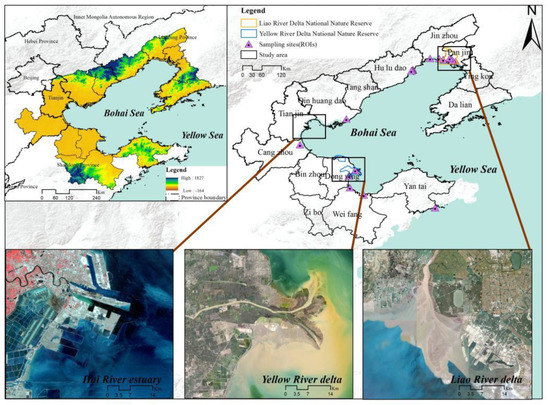
Figure 1.
Location of the study area.
2.2. Data Preprocessing
All of the available archived standard level 1 terrain corrected (L1T) orthorectified Landsat imagery (~430 images) for the study area were used to generate annual S. salsa maps for the period from 1990 to 2020 based on the GEE platform. The observations of Landsat images in path/row (121–122,32–33) from 1 June 1990 to 31 October 2020 were chosen. The image data were selected from August to early November because the spectral characteristics of S. salsa differ from those of other coastal wetland vegetation types in this period [16]. Low-quality observations, including those with clouds (more than 10%), cloud shadows, cirrus, snow/ice, and scan-line corrector (SLC)-off gaps, were addressed by using the F-mask band and were not used in the data analyses [37]. The Landsat imagery preprocessing tasks were conducted as described in the flow chart (Figure 2). Furthermore, the artificial coastlines were delineated through visual interpretation. The topography data were obtained from the Geospatial Data Cloud (http://www.gscloud.cn/) and accessed on 30 July 2021. The daily meteorological data from 1990 to 2020 were collected from the China Meteorological Data Network (http://data.cma.cn/) and accessed on 30 July 2021.
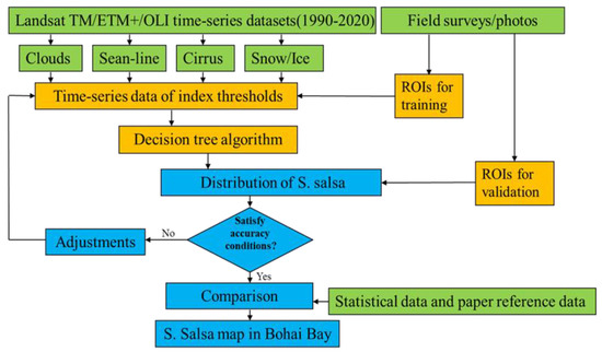
Figure 2.
Flow chart of mapping S. salsa using Landsat time-series images from 1990 to 2020.
A robust decision tree algorithm was used to produce annual S. salsa maps from 1990 to 2020 at a 30-m spatial resolution. Decision tree classification is a method used to conduct classification rules and carry out remote sensing classifications through summaries of expert knowledge and experience, simple mathematical statistics, and inductive methods [38]. The main features in the study area were first classified as follows: non-vegetation and vegetation. Non-vegetation mainly includes water bodies, mudflats, and buildings. For vegetation, S. salsa was distinguished from the other land cover types based on its spectral characteristics from August to early November in each year. By setting the conditions in the decision tree classification method according to the spectral reflectance differences of different features, these indices were used to identify S. salsa (NDVI > 0.07, Red < 0.109, SWIR1 > 0.03, SWIR2 < 0.05, NIR*Red < 0.0109, Green–Red < 0.006, NIR-Red < 0.07) and (Green–Red)/(Green + Red) < 0.04), which could be distinguished from other features [39,40]. Based on the S. salsa results from the GEE platform, the final results for the S. salsa distributions were obtained by verification with field surveys to strengthen the positional accuracies. Several land types, such as ponds and salt pans, affected the overall accuracy of the results, as they have similar characteristics: low vegetation density and seasonal inundation. Visual adjustments were used to modify and remove interference to improve the accuracy. The annual S. salsa maps in the Bohai Bay region were produced by using the abovementioned imagery, algorithm, and GEE platform. A region of interest (ROI) approach and field surveys were combined to verify and assess the accuracy of the maps. Two times duplicated field sample were conducted to produce ROI points in October 2018 and October 2019, respectively, which followed the same route and sample points (Figure 1). The study area was divided into S. salsa regions and regions with no S. salsa, and the ROI points (120 in three main areas) were generated with field surveys [30]. The location of the sites where mainly distributed in Liao River delta, Yellow River delta and Hai River estuary was showed in Figure 1. The final points were checked by using field surveys and photos, and invalid points were excluded. Three typical sampling areas where S. salsa is densely distributed were selected to study the S. salsa distributions and are shown in Figure 3. Then, a confusion matrix was used to evaluate the overall accuracy and kappa coefficients of the results, for which the overall accuracy and kappa coefficients of S. salsa maps were all above 85.50% and 0.85, respectively.
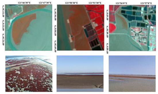
Figure 3.
Locations of selected typical regions of interest of S. salsa.
2.3. Analysis of Pattern Fragmentation
Quantifying the dynamics of the S. salsa distributions under natural and anthropogenic changes is critical for understanding coastal sustainability. Landscape metrics are generally applied to describe landscape patterns at various scales [41]. Based on the meanings of landscape metrics [42], the largest patch index (LPI), patch density (PD), landscape shape index (LSI), and aggregation index (AI) were chosen. LPI represented the percentage of the largest patch area to the total area of types. The values reflected the intensity and frequency of the disturbance. PD reflected the degree of patch fragmentation, as the higher the value the more serious the fragmentation of patches. LSI reflected the complexity of patch shape, as the higher the value the more complex the patch shape. AI reflected the degree of patch dispersion, as the higher the value the higher the degree of patch aggregation [43]. The landscape metrics were calculated using FRAGSTATS 4.2 (University of Massachusetts in Amherst, Amherst, MA, USA).
2.4. Analysis of Influencing Factors
Multivariate data analysis techniques, such as principal component analysis (PCA) and the logistic regression model (LRM), have been recognized as effective methods for analyzing the relationships among voluminous quantities of data [44]. To explore the key natural influencing factors for the S. salsa changes, we used mutually complementary methods in the analysis. The details are as follows:
The correlation coefficients of the independent variables were analyzed firstly by the Pearson correlation. Then, PCA maximizes the correlations among the original variables and forms new variables that are mutually orthogonal or uncorrelated [45]. PCA can reduce complex data to a new set of variables, as the number of principal components is less than or equal to the number of original variables and provides linear combinations of the original dataset after decreasing the number of variables in the dataset. The identification and observation of the variation sources is enabled by PCA. In this paper, the correlation coefficients of the independent variables are shown in Figure 4. The results show that the independent variables were correlated with each other, and the PCA method was necessary to analyze the major influencing factors. The data sufficiency for variable analysis was analyzed by the Kaiser-Meyer-Olkin Measure (KMO) and Bartlett’s test of sphericity. The results indicated that the KMO test (0.654) value that was larger than 0.5 indicated adequate data. The Bartlett’s sphericity test (p < 0.001) showed a high degree of relationship for each factor, and the data were suitable for further analysis.
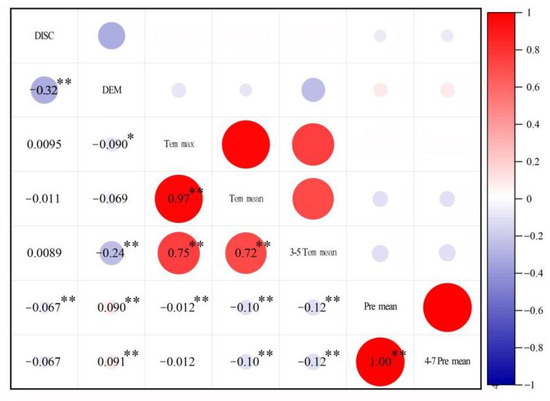
Figure 4.
The correlation coefficients of the independent variables. (Note: * and ** represent 5% and 1% significance, respectively.)
A logistic regression model can be applied to the model and examine the relationships of several independent variables (Xn) to a dichotomous, single dependent variable (Y), which indicates the occurrence or nonoccurrence of an event [46,47]. The method yields the probability in each location based on the influencing factors and quantifies the relationships among the different degradation conditions and their drivers. In this study, the independent variables were defined as the natural influencing factors for S. salsa changes. The dependent variables indicated either disappear or appear. The disappeared area of S. salsa due to the transition into other land use types was removed because the occupied parts cannot be restored in the future. S. salsa area was disappeared by natural factors and was discussed only in logistic regression model. An amount of 630 samples were selected for use in the logistic regression model. All samples were divided into modeling samples (60%) and independent test samples (40%); 70% of the modeling samples were randomly selected as training samples and 30% as verification samples. Five repetitions were carried out, and the optimal intermediate model was obtained by stepwise regression (α < 0.05). The binary logistic regression model is conducted as follows:
where P(Y = 1) is the probability of S. salsa degradation; β0 is the fixed intercept; x1, …, xn are independent variables, which represent the various drivers that influence the changes in S. salsa; β1, …, βn are the coefficients of each independent variable; ε is the error.
The logistic transformation of P (Y = 1) is as follows:
where the P(Y = 1)/[1-P(Y = 1)] values indicate the odds of changes in S. salsa, that is, the ratio of the probability that Y = 0 to the ratio of the probability that Y = 1.
2.5. Selection on Influencing Factors
The natural factors mainly include both the climate and topography in coastal zones [48]. The selection of the independent variables was achieved from the results of previous studies and from the results of field surveys, and these variables were temperature, precipitation, elevation, and salinity stress. Seven variables were selected and are listed in Table 1. The terrain on the seaward side was constantly silted up in the coastal zone, which resulted in weak impacts from seawater tidal invasion on S. salsa. The DEM represented the elevation after sediment deposition in the tidal flat. The distance to the coastline represented the topographic features and salinity gradients [49,50,51]. The S. salsa distribution was located farther away from the coastline, and the salinity and degree of inundation were higher. In particular, the temperature and precipitation for S. salsa during the germination and growth stages were focused on from March to May and April to July, which also indirectly affected the salinity in the study area. The human activities were summarized as occupations, essentially, the land use types were changed. These were not further analyzed in terms of their details.

Table 1.
List of the variables included in the logistic regression.
3. Results
3.1. Area Changes of S. salsa from 1990 to 2020
The S. salsa areas continued to decrease from 1990 to 2020 in the study area (Figure 5). The S. salsa areas decreased from 692.93 km2 in 1990 to 51.04 km2 in 2020. Although the areas with S. salsa have fluctuated in the past 31 years, the overall area has decreased by 92.63%. Figure 6 shows that the spatial distributions of S. salsa were organized into three main parts over the past 31 years: the Liao River Delta (Liaoning Province), Yellow River Delta (Shandong Province), and Hai River Estuary (Hebei Province, Tianjin). The results showed that the overall trends of the S. salsa areas in the Bohai Bay region were consistent with the trend of the S. salsa area in the Yellow River Delta (Figure 5). The Yellow River Delta had the largest S. salsa area in the study area. The S. salsa areas decreased rapidly by approximately 376 km2 from 1990 to 1996. The changes in the S. salsa areas were relatively stable during 1997–2004. The decreasing trend has continued until 2020. The Liao River Delta had the second largest area of S. salsa in the study area, and the S. salsa area decreased by approximately 96.48 km2 from 1990 to 2000. The S. salsa area increased by 14.78 km2 from 2007 to 2014, but the area significantly shrank to 8.78 km2 by 2019. Fortunately, the S. salsa area significantly increased in 2020. For the Hai River estuary, the maximum S. salsa area was 5.18 km2, and S. salsa has almost completely disappeared since 1998. Reclamation activities started in the Hai River estuary in 1978, and the development projects were characterized by few projects but large areas. The landscape patterns of the Hai River Estuary were transformed by the human utilization of natural wetlands.
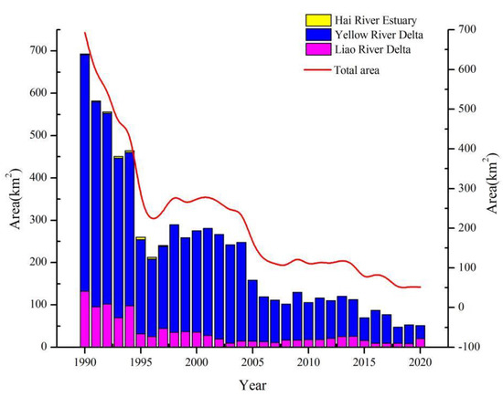
Figure 5.
Dynamic changes in the S. salsa areas for each year.
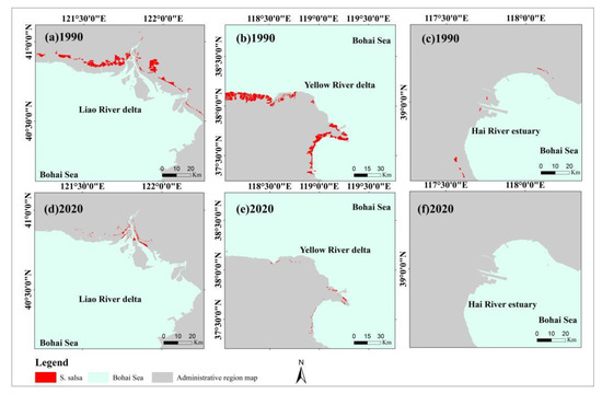
Figure 6.
The administrative region map in the 1990s and S. salsa areas in Bohai Bay in 1990 and 2020: (a) Liao River Delta in 1990, (b) Yellow River Delta in 1990, (c) Hai River Estuary in 1990, (d) Liao River Delta in 2020, (e) Yellow River Delta in 2020, and (f) Hai River Estuary in 2020.
3.2. Landscape Pattern Changes of S. salsa
Figure 7 shows the S. salsa changes in the landscape pattern metrics in the Bohai Bay region from 1990 to 2020. The PD values fluctuated slightly and increased by 0.88 times from 1990 to 2015. However, the PD values increased from 0.62 in 2016 to 4.80 in 2020, which is an increase of 4.18 times. The AI values of the results fluctuated slightly, which showed a declining trend for the patch aggregation level during the study period. Notably, the lowest AI value was 91.07 in 2016, which indicated that the patch dispersion degree of S. salsa was significant. The AI values increased slightly, which indicated that the S. salsa patches exhibited an aggregation trend. The LSI is an indicator that reflects the complexity of landscape patch shapes. Although the LSI values from 2010 to 2018 were slightly higher than those in other years, the overall trend of the LSI values was relatively stable. The LPI values fluctuated significantly in the past several years, which indicated that the S. salsa patches were disturbed by interference. One of the reasons was restricted the disturbance of human activities, and the distribution of S. salsa increased when the natural conditions of its growth was suited in the year. However, the changes of natural factors per year was very uncertain, which caused the change of LPI values greatly. However, overall trends demonstrated that the landscape fragmentation of S. salsa had intensified. The landscape pattern metrics showed that the landscape fragmentation of S. salsa exhibited periodic fluctuations, but it continued to become fragmented during the study period.
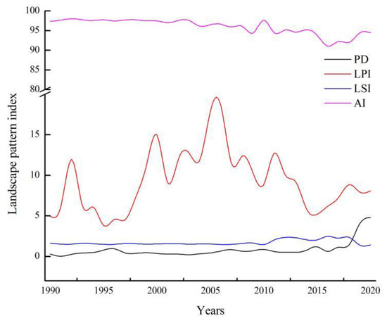
Figure 7.
Landscape pattern changes for S. salsa for each year.
3.3. Spatial Distributions of S. salsa in the National Nature Reserves
The study area includes the Liao River Delta and Yellow River Delta National Nature Reserves (NNR), which are the two core areas containing S. salsa distributions. Four phases of typical changes in S. salsa were analyzed in both National Nature Reserves. In the Liao River Delta NNR, S. salsa was mainly distributed on both sides of the tidal flat in the Liao River Estuary (Figure 8a). Until 2000, S. salsa experienced a significant decline west of the Liao River Delta NNR because the construction of the key water project in the delta began in 1988 and the development of cultivated land was mostly completed in 2000 (Figure 8b). The S. salsa distributions on both sides of the Liao River Estuary almost completely disappeared, with the smallest area in 2017, and the habitat suitable for S. salsa was seriously threatened (Figure 8c). The protection and restoration projects of the “red beach” in the Liao River Delta have been implemented since 2018. The S. salsa distribution increased, which was related to the improvement of its habitat in the Liao River Delta NNR (Figure 8d). In the Yellow River Delta NNR, S. salsa has lost 50 km2 of area in the past 31 years. Many reclamation areas have been added in the north, middle, and south parts of the delta since 1994 (Figure 8e). Only the S. salsa regions in the NNR of the Yellow River Delta and west side were not developed, and the remaining areas became reclamation areas, which caused the S. salsa area to decrease until 2004 (Figure 8f). S. salsa remained undeveloped only in the Yellow River Delta NNR, which decreased to 86.32 km2 in 2014. The area actually continued to shrink from 2014 to 2020 (Figure 8g−h). The change rate of S. salsa was higher outside NNR than inside (Figure 9). The number of years with an increasing trend of S. salsa inside NNR was more than that outside. Actually, the human activities had been controlled effectively inside NNR, and the changes were mainly caused by the influence of natural factors.
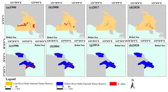
Figure 8.
Dynamic changes in S. salsa in NNR (the administrative region map in the 1990s): (a–d) Liao River Delta NNR in 1990, 2000, 2017, 2020, respectively. (e–h) Yellow River Delta NNR in 1990, 2004, 2014, 2020, respectively.
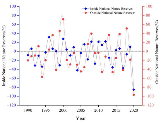
Figure 9.
Change rate of S. salsa inside and outside National Nature Reserves.
3.4. Influencing Factors of S. salsa Changes
Natural and anthropogenic factors have impacts on the dynamic changes of the S. salsa distributions in the study area. The results showed that the decreasing trend of S. salsa was caused by anthropogenic activities; 348.80 km2 of this area was converted to other anthropic land use categories, which accounted for 54.34% of the total change. While 293.09 km2 was degraded to bare land, which accounted for 45.66% of the total change (Figure 10). The occupation by human activities, which refers to the changes in land use type, was identified as the main driving factor for the S. salsa changes in the study area. On the one hand, this occupation contained cultivated land, aquaculture, and construction projects. The development due to earlier activities directly and indirectly occupied the habitats of S. salsa. On the other hand, water cycles were cut off by facilities between the sea and land at the tidal ditch, and the hydrodynamic conditions favorable for the growth conditions of S. salsa were changed. The natural influencing factors of the S. salsa changes due to topography and climate will be analyzed in detail in the next section.
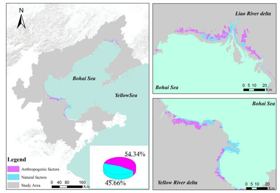
Figure 10.
Influencing factors for the S. salsa changes in the study area.
The results show that the seven independent variables were correlated with each other, and the PCA method was necessary to analyze the major influencing factors. The eigenvalues for all linear components before and after rotation extraction are depicted in Table 2. The cumulative variance of the principal components was 89.00%, the first component explained 71.06%, and 20.60% was explained by the second component. The most significant principal components for explaining the amounts of variance were the first and second principal components.
Table 2.
Total variance explained.
The factor loading values after rotation are vital for explaining the PCA results. The principal components were rotated to obtain a better understanding and explanation of the data. Only those components with eigenvalues greater than 1 were recognized as principal components, and varimax rotation acted as the criterion. The eigenvalues after rotation are shown in Table 2. After rotation, the variance of the first principal component decreased by 0.33%, from 71.06% to 70.73%. The variances of the other principal components increased by 0.33%. This result indicated that PC1 is more closely correlated with the variables than the other components after rotation. As shown in Table 2 and Table 3, PC1 explained approximately 71.73%, which had positive loadings (e.g., 0.999 with 4–7 Premean, 0.998 with Premean, 0.998 with Temmax, 0.994 with Temmean, and 0.984 with 3–5 Temmean). PC1 was related to the reduction of S. salsa due to natural factors. The second factor explained approximately 18.27% of the total variance and had positive loadings with DEM (0.805) and DISC (−0.785). The climate factors, including precipitation and temperature, were critical for the dynamic changes in S. salsa.
Table 3.
Original and rotated component matrices.
The logistic regression results are summarized in Table 4 and were significant at the 1% level, which illustrate the joint significance of the variables. The explanation of the prediction of the regression model was 0.746, which indicated that it accurately predicted approximately 74.6%. Among the two types of variables, the characteristics of Premean, 4–7 Premean, Temmean 3–5 Temmean, Temmax, DEM, and distance to coastline had significant impacts on the changes in S. salsa. The contribution rates of the driving factors (Wald) in order were Tmean, 3–5 Tmean, 4–7 Premean, DISTC, Tmax, Premean, and DEM. The equation of the model is defined as follows:
Table 4.
Logistic regression results of the driving factors for the changes in S. salsa.
Precipitation, temperature, elevation, and distance to the coastline were considered to be the major influencing factors for the S. salsa changes. The results showed that the temperatures in March may have a key impact on the seed germination of S. salsa, but the annual average temperature had slight effects. The inter-annual variations in precipitation have fluctuated greatly over the past 31 years. The reductions in rainfall have had an impact on the estuarine water inflows, and the water conditions for S. salsa growth were not satisfied in the tidal flats. Drought, especially during the key sprouting periods (e.g., April to June in each year), led to low seedling emergence rates of S. salsa. The terrain (DEM) was an important factor that influenced the changes in S. salsa distributions. Large amounts of sediment deposition elevated the topography to a level suitable for S. salsa growth in the tidal flats, which promoted the growth of most saline vegetation. The distance to the coastline indicated the salinity, degree of inundation, and tidal influence. These factors were beyond the tolerance range of S. salsa growth, and S. salsa had no suitable habitat. S. salsa seeds have a certain degree of tolerance to tides, which are conducive to their germination in the soil of wetland habitats with complex hydrological conditions.
4. Discussion
4.1. Annual Monitoring Using Landsat Data and the GEE Platform
The feasibility and reliability of the S. salsa maps at a 30-m spatial resolution were demonstrated by using Landsat TM/ETM + /OLI imagery and the GEE platform. The overall accuracy and kappa coefficients of the annual S. salsa maps were above 85.50% and 0.85 (OA > 85.50%, Kappa > 0.85), respectively. In addition, the classification results obtained from the GEE platform and combined with many field sampling sites as to improve and verify the accuracy of the S. salsa maps. In this study, the images mentioned above were selected for the period from August to early November of each year, and the S. salsa plants showed a significant purplish red color, which had specific spectral characteristics. All available images were significantly improved in the period used and effectively distinguished S. salsa from other vegetation types. However, the growth stages of S. salsa changed quickly every year, and the number of good-quality observations was limited. To reduce the uncertainties, the number of sampling sites were produced as much as possible to evaluate the S. salsa maps by combining field surveys, photos, and previous studies. The results of other studies and results in this study were compared, and it showed that the results were consistent on the overall change trend of S. salsa. For the Liao River Delta, the results for the S. salsa areas in Guan’s research were 7.4 km2, 15.34 km2, 18.69 km2, and 8.41 km2 in 2007, 2009, 2012, and 2016, respectively [52], and the results in our study were 11.29 km2, 16.68 km2, 20.61 km2, and 9.46 km2, respectively. For the Yellow River Delta, the S. salsa areas in Liu’s research were 664.29 km2, 277.41 km2, and 196.93 km2 in 1994, 2004, and 2014, respectively [35], and the results in our study were 362.26 km2, 232.88 km2, and 86.32 km2. The differences were mainly caused by the observations of tide coastline locations, which were visually interpreted from a single no-cloud image for each period to define the S. salsa regions [4]. Furthermore, the results of S. salsa in this study were extracted for each year during 1990 to 2020, and the consistency was higher in continuous time series. The classification method had differences. The results of this paper used decision tree algorithm, and the algorithm has been widely used and proved to be systematic and complete so that more fragmented patches were extracted in this study [27].
4.2. Limitations and Future Studies
Occupation by human activities was identified as one of the major factors that affected the S. salsa distributions in coastal zones [28,53]. The essential effect of these occupations was only that the land use type was changed by human activities, which blocked the material and energy exchange between the sea and land and led to shrinkage of the suitable habitats for S. salsa. Thus, only the natural influencing factors were discussed in detail in this study. Precipitation and temperature were discussed as the main driving factors of climate change. Precipitation was one of the main sources for the water conditions necessary for S. salsa growth. In addition, the increased temperatures affected the evaporation of water and salinity levels in the tidal flats. Soil water is considered to be another driving factor for plant vegetation succession, and the soil water levels at different depths serve as a major source for sustaining the growth of plants and population stability [9,54]. Meanwhile, most of the sediment deposition led to terrain changes in the tidal-flat areas, and S. salsa was subjected to inappropriate salinity levels, which resulted in restrictions on S. salsa growth. The process of micro-topography influences is actually complex and will be further analyzed in future works. The dynamic changes in S. salsa distributions and the factors that affect their changes in this study were studied at the regional scale. Laboratory tests were not conducted, and it is impossible to further study the effects on seed germination and the physiological mechanism of S. salsa growth under different conditions. Further analyses of laboratory tests will be carried out in future studies. The distance to the coastline and the sea indirectly reflected the changes in the salinity gradient [55], among which the salinity gradually increased with increasing distance to the coastline. Therefore, the distance to the coastline was selected to represent the change in salinity. Furthermore, a number of RS products with higher spatial and temporal resolutions have been applied in recent years, such as Sentinel-2 and World 3, and annual S. salsa maps with higher accuracies in short time series will be generated by improving the algorithms.
4.3. Potential Applications for S. salsa Conservation
S. salsa is a dominant species in coastal wetlands and constitutes a natural ecological barrier in coastal zones [16]. Restoring S. salsa can effectively balance the ecological environment and curb coastal soil desertification so that the biodiversity, and the sustainable development of the coastal economy are promoted [56]. In this study, the algorithms, time series Landsat imagery, and GEE platform could maximize the use of the available images and have advantages in generating annual maps of other vegetation types to monitor the dynamic changes in a specified species. In addition, our approach provided a tool for accurate and objective assessments of the changes in S. salsa at appropriate spatial-temporal scales, which potentially supported conservation policies and management in long-term series. It is crucial to understand and protect coastal wetlands [57].
In the detailed analysis, the change of S. salsa distribution has been shrinking [16]. The occupation activities (e.g., reclamation, aquaculture, and agriculture) and natural changes had effects on S. salsa distribution [58]. An amount of 54.34% of the total change are related to the human interference and the impact of policies. The construction projects in the study area should be appropriately controlled. Actually, the NNR areas played a crucial role in maintaining the change trend of S. salsa, indicating that trends can be determined according to the national or regional policy. With the adjustment of the regulations on the management of NNR areas, human destructive activities are prohibited or restricted. Liao River Delta and Yellow River Delta NNR have been established since 1986 and 1992 [34], respectively. The establishment periods of the NNR basically coincided with the temporal scale we studied. Although the change of S. salsa has fluctuated, it will contribute to the recovery of S. salsa with the gradual improvement of the NNR management system. Besides, the notice on strengthening the protection and management of wetlands that was issued by the General Office of the State Council, as a policy for wetland conservation, has been promulgated since 2004 (http://www.gov.cn/), and accessed on 1 December 2021.
The protection and restoration of S. salsa is a complex project that must be managed scientifically and systematically from different perspectives, such as water and salinity regulation, soil nutrition, and ecological balance [9]. The regions where S. salsa had previously appeared were determined in our study and were the potential suitable habitats for S. salsa growth as restoration areas in the future. According to the results of natural influencing factors, precipitation, temperature, elevation, and distance to the coastline had an impact on the distribution of S. salsa. Therefore, we put forward measures for these aspects in ecological restoration processes [59]. Water Diversion Projects can be built to satisfy freshwater demand and reduce salinity in soil. Fresh water resources can be saved by adjusting terrain, as such a grid device in the tidal-flat area was built to preserve water, and this water was irrigated to reduce salinity, which was the potential measures for S. salsa restoration. The measures mentioned above all had references for coastal wetland vegetation restoration.
5. Conclusions
S. salsa has significant ecological, ornamental, and socioeconomic values for wetland vegetation in coastal zones. Monitoring the dynamic changes in S. salsa distributions at the regional scale is meaningful for coastal wetland conservation. The present study generated annual S. salsa maps in the Bohai Bay region at 30-m resolution over the last 31 years by using a decision tree algorithm and time series Landsat data on the GEE platform, which provided a guideline for evaluating the changes in a specific species at a regional scale. The spatial-temporal dynamic changes in S. salsa were explored, and the key natural influencing factors for the changes in S. salsa were analyzed by the PCA method and logistic regression model. The results showed that the spatial distributions of S. salsa were organized into three main parts: the Liao River Delta, Yellow River Delta, and Hai River Estuary. The overall S. salsa area decreased by 92.63%. The landscape fragment of S. salsa has showed an increasing trend in the past 31 years. The occupation by human activities that led to degradation accounted for 54.90%, and the remainder of the degradation resulted from natural influencing factors. Precipitation, temperature, elevation, and distance to the coastline were recognized as the major factors affecting S. salsa changes. S. salsa, as an annual herb, has changed rapidly, and the dynamic was monitored difficultly. This study has demonstrated the potential of the described method for monitoring the dynamic annual changes in S. salsa in a long-term series. Our annual maps and driver factor analysis are likely to provide vital information for S. salsa conservation and restoration.
Author Contributions
Conceptualization, Y.H., M.L. and H.Y.; methodology, H.Y; software, H.Y.; validation, C.L. and H.Y.; formal analysis, H.Y.; investigation, M.L., C.L. and H.Y.; resources, M.L., C.L., Y.C. and H.Y.; data curation, H.Y.; writing—original draft preparation, H.Y.; writing—review and editing, Y.C., M.L. and C.L.; visualization, H.Y.; supervision, Y.H., Y.C. and M.L.; project administration, Y.H. and M.L.; funding acquisition, Y.H., M.L. and C.L., M.L. and C.L. have equal contribution. All authors have read and agreed to the published version of the manuscript.
Funding
This research was funded by National Natural Science Foundation of China, grant number (Nos. 32071580, 41871192, 41730647).
Data Availability Statement
The data presented in this study are available on request from the corresponding author.
Conflicts of Interest
The authors declare no conflict of interest.
References
- Thorslund, J.; Jarsjo, J.; Jaramillo, F.; Jawitz, J.W.; Manzoni, S.; Basu, N.B.; Chalov, S.R.; Cohen, M.J.; Creed, I.F.; Goldenberg, R.; et al. Wetlands as large-scale nature-based solutions: Status and challenges for research, engineering and management. Ecol. Eng. 2017, 108, 489–497. [Google Scholar] [CrossRef]
- Camacho-Valdez, V.; Ruiz-Luna, A.; Ghermandi, A.; Nunes, P.A.L.D. Valuation of ecosystem services provided by coastal wetlands in northwest Mexico. Ocean. Coast. Manag. 2013, 78, 1–11. [Google Scholar] [CrossRef]
- Gedan, K.B.; Silliman, B.R.; Bertness, M.D. Centuries of Human-Driven Change in Salt Marsh Ecosystems. Annu. Rev. Mar. Sci. 2009, 1, 117–141. [Google Scholar] [CrossRef] [Green Version]
- Wang, X.; Xiao, X.; Zou, Z.; Chen, B.; Ma, J.; Dong, J.; Doughty, R.B.; Zhong, Q.; Qin, Y.; Dai, S.; et al. Tracking annual changes of coastal tidal flats in China during 1986–2016 through analyses of Landsat images with Google Earth Engine. Remote Sens. Environ. 2020, 238, 110987. [Google Scholar] [CrossRef] [PubMed]
- Peter, C.; Lerato, S.K. Montane Palustrine Wetlands of Lesotho: Vegetation, Ecosystem Services, Current Status, Threats and Conservation. Wetlands 2021, 41, 67. [Google Scholar] [CrossRef]
- Zhang, X.; Zhang, Z.; Wang, W.; Fang, W.; Chiang, Y.; Liu, X.; Ju, H. Vegetation successions of coastal wetlands in southern Laizhou Bay, Bohai Sea, northern China, influenced by the changes in relative surface elevation and soil salinity. J. Environ. Manag. 2021, 293, 112964. [Google Scholar] [CrossRef] [PubMed]
- Lu, Y.; Fernanda, A.M.; Chengrong, C. Resource stoichiometry, vegetation type and enzymatic activity control wetlands soil organic carbon in the Herbert River catchment, North-east Queensland. J. Environ. Manag. 2021, 296, 113183. [Google Scholar] [CrossRef]
- Püttker, T.; Meyer-Lucht, Y.; Sommer, S. Effects of fragmentation on parasite burden (nematodes) of generalist and specialist small mammal species in secondary forest fragments of the coastal Atlantic Forest, Brazil. Ecol. Res. 2008, 23, 207–215. [Google Scholar] [CrossRef]
- An, Y.; Gao, Y.; Zhang, Y.; Tong, S.; Liu, X. Early establishment of Suaeda salsa population as affected by soil moisture and salinity: Implications for pioneer species introduction in saline-sodic wetlands in Songnen Plain, China. Ecol. Indic. 2019, 107, 105654. [Google Scholar] [CrossRef]
- Tian, Y.; Luo, L.; Mao, D.; Wang, Z.; Li, L.; Liang, J. Using Landsat images to quantify different human threats to the Shuangtai Estuary Ramsar site, China. Ocean. Coast. Manag. 2017, 135, 56–64. [Google Scholar] [CrossRef]
- Guan, B.; Yu, J.; Wang, X.; Fu, Y.; Kan, X.; Lin, Q.; Han, G.; Lu, Z. Physiological Responses of Halophyte Suaeda salsa to Water Table and Salt Stresses in Coastal Wetland of Yellow River Delta. CLEAN-Soil Air Water 2011, 39, 1029–1035. [Google Scholar] [CrossRef]
- Sun, Z.; Song, H.; Sun, W.; Sun, J. Effects of continual burial by sediment on morphological traits and dry mass allocation of Suaeda salsa seedlings in the Yellow River estuary: An experimental study. Ecol. Eng. 2014, 68, 176–183. [Google Scholar] [CrossRef]
- Cui, H.; Bai, J.; Du, S.; Wang, J.; Keculah, G.N.; Wang, W.; Zhang, G.; Jia, J. Interactive effects of groundwater level and salinity on soil respiration in coastal wetlands of a Chinese delta. Environ. Pollut. 2021, 286, 117400. [Google Scholar] [CrossRef] [PubMed]
- Hao, X.; Lei, D.; Ying, H. An Analysis of Dynamic Monitoring and Landscape Pattern Change of Suaeda salsa Wetlands in Panjin Using Remote Sensing Technology. Wetl. Sci. Manag. 2017, 13, 31–36. [Google Scholar] [CrossRef]
- Song, L.; Mou, X.; Liu, X. Anthropogenic effect on wetland vegetation growth in the Yellow River Delta. Ecol. Environ. Sci. 2019, 28, 2307–2314. [Google Scholar]
- Zhang, J.; Zhang, Y.; Lloyd, H.; Zhang, Z.; Li, D. Rapid Reclamation and Degradation of Suaeda salsa Saltmarsh along Coastal China’s Northern Yellow Sea. Land 2021, 10, 835. [Google Scholar] [CrossRef]
- Guo, J.; Chen, Y.; Lu, P.; Liu, M.; Sun, P.; Zhang, Z. Roles of endophytic bacteria in Suaeda salsa grown in coastal wetlands: Plant growth characteristics and salt tolerance mechanisms. Environ. Pollut. 2021, 287, 117641. [Google Scholar] [CrossRef] [PubMed]
- Wang, S.; Liu, Y.; Chen, L.; Yang, H.; Wang, G.; Wang, C.; Dong, X. Effects of excessive nitrogen on nitrogen uptake and transformation in the wetland soils of Liaohe estuary, northeast China. Sci. Total Environ. 2021, 791, 148228. [Google Scholar] [CrossRef]
- Yang, C.; Lv, D.; Jiang, S.; Lin, H.; Sun, J.; Li, K.; Sun, J. Soil salinity regulation of soil microbial carbon metabolic function in the Yellow River Delta, China. Sci. Total Environ. 2021, 790, 148258. [Google Scholar] [CrossRef]
- Subrina, T.; Medeiros, S.C.; Arvind, S. Consistent Long-Term Monthly Coastal Wetland Vegetation Monitoring Using a Virtual Satellite Constellation. Remote Sens. 2021, 13, 438. [Google Scholar] [CrossRef]
- Xie, Z.; Phinn, S.R.; Game, E.T.; Pannell, D.J.; Hobbs, R.J.; Briggs, P.R.; Beutel, T.S.; Holloway, C.; McDonald-Madden, E. Using Landsat observations (1988–2017) and Google Earth Engine to detect vegetation cover changes in rangelands—A first step towards identifying degraded lands for conservation (vol 232, 111317, 2019). Remote Sens. Environ. 2020, 241, 111317. [Google Scholar] [CrossRef]
- Wang, X.X.; Xiao, X.M.; Zou, Z.H.; Hou, L.Y.; Qin, Y.W.; Dong, J.W.; Doughty, R.B.; Chen, B.Q.; Zhang, X.; Cheng, Y.; et al. Mapping coastal wetlands of China using time series Landsat images in 2018 and Google Earth Engine. Isprs J. Photogramm. Remote Sens. 2020, 163, 312–326. [Google Scholar] [CrossRef] [PubMed]
- Villa, P.; Giardino, C.; Mantovani, S.; Tapete, D.; Vecoli, A.; Braga, F. Mapping Coastal and Wetland Vegetation Communities Using Multi-temporal Sentinel-2 Data. Int. Arch. Photogramm. Remote Sens. Spat. Inf. Sci. 2021, 43, 639–644. [Google Scholar] [CrossRef]
- Amani, M.; Brisco, B.; Afshar, M.; Mirmazloumi, S.M.; Mahdavi, S.; Mirzadeh SM, J.; Huang, W.; Granger, J. A generalized supervised classification scheme to produce provincial wetland inventory maps: An application of Google Earth Engine for big geo data processing. Big Earth Data 2019, 3, 378–394. [Google Scholar] [CrossRef]
- Hütt, C.; Koppe, W.; Miao, Y.; Bareth, G. Best Accuracy Land Use/Land Cover (LULC) Classification to Derive Crop Types Using Multitemporal, Multisensor, and Multi-Polarization SAR Satellite Images. Remote Sens. 2016, 8, 684. [Google Scholar] [CrossRef] [Green Version]
- Abdi, A.M. Land cover and land use classification performance of machine learning algorithms in a boreal landscape using Sentinel-2 data. GIScience Remote Sens. 2019, 57, 1–20. [Google Scholar] [CrossRef] [Green Version]
- Deslandes, S.; Grenier, M.; Belanger, L.; Lacroix, G.; Zingraff, V. The Wetland Conservation Atlas of the St.Lawrence Valley produced from decision tree classifications of RADARSAT and Landsat images. In Proceedings of the IEEE International Geoscience and Remote Sensing Symposium (IGARSS 2002)/24th Canadian Symposium on Remote Sensing, Toronto, ON, Canada, 24–28 June 2002; pp. 2893–2895. [Google Scholar]
- Gong, P.W.; Yu, L.J. Finer resolution observation and monitoring of global land cover: First mapping results with Landsat TM and ETM+ data. Int. J. Remote Sens. 2013, 34, 2607–2654. [Google Scholar] [CrossRef] [Green Version]
- Sun, S.; Zhang, Y.; Song, Z.; Chen, B.; Zhang, Y.; Yuan, W.; Chen, C.; Chen, W.; Ran, X.; Wang, Y. Mapping Coastal Wetlands of the Bohai Rim at a Spatial Resolution of 10 m Using Multiple Open-Access Satellite Data and Terrain Indices. Remote Sens. 2020, 12, 4114. [Google Scholar] [CrossRef]
- Chen, B.; Xiao, X.; Li, X.; Pan, L.; Doughty, R.; Ma, J.; Dong, J.; Qin, Y.; Zhao, B.; Wu, Z. A mangrove forest map of China in 2015: Analysis of time series Landsat 7/8 and Sentinel-1A imagery in Google Earth Engine cloud computing platform. ISPRS J. Photogramm. Remote Sens. 2017, 131, 104–120. [Google Scholar] [CrossRef]
- Qu, X.; Liu, M.; Li, C.; Yin, H.; Chang, Y.; Hu, Y. Evaluation and prediction of the comprehensive carrying capacity in the Bohai ring region. Chin. J. Soil Sci. 2020, 51, 552–560. [Google Scholar] [CrossRef]
- Zhang, T.; Chang, J.; Ma, Y.; Sun, Y.; Liu, C. Study on the Evolution Characteristics of Coastal Wetlands of Bohai Sea in Shandong Province under the Influence of Human Activities. J. Coast. Res. 2020, 105, 28–32. [Google Scholar] [CrossRef]
- Ding, X.; Shan, X.; Chen, Y.; Jin, X.; Rahman, F. Dynamics of shoreline and land reclamation from 1985 to 2015 in the Bohai Sea, China. J. Geogr. Sci. 2019, 29, 2031–2046. [Google Scholar] [CrossRef] [Green Version]
- Yin, H.; Hu, Y.; Liu, M.; Li, C.; Lv, J. Ecological and Environmental Effects of Estuarine Wetland Loss Using Keyhole and Landsat Data in Liao River Delta, China. Remote Sens. 2021, 13, 311. [Google Scholar] [CrossRef]
- Liu, K.; Yan, J.; Zou, Y.; Song, G.; Zheng, J.; Cui, B. Dynamics of Spatial and Temporal Distribution of Suaeda salsa Salt Marshes in the Yellow River Delta. Wetl. Sci. 2015, 13, 696–701. [Google Scholar]
- Mu, X. Research on the relationship between the evolution process of reclamation, shoreline and wetland changes of Tianjin Binhai new area. Ph.D. Thesis, Tianjin University, Tianjin, China, 2014. [Google Scholar]
- Bedard, F.; Reichert, G.; Dobbins, R.; Trepanier, I. Evaluation of segment-based gap-filled Landsat ETM plus SLC-off satellite data for land cover classification in southern Saskatchewan, Canada. Int. J. Remote Sens. 2008, 29, 2041–2054. [Google Scholar] [CrossRef]
- Peng, Y.; He, G.; Wang, G.; Cao, H. Surface Water Changes in Dongting Lake from 1975 to 2019 Based on Multisource Remote-Sensing Images. Remote Sens. 2021, 13, 1827. [Google Scholar] [CrossRef]
- Mu, M. Inversion Model Study of Suaeda salsa Biomass Based on Hyperspectral Remote Sensing. Master’s Thesis, Dalian Ocean University, Dalian, China, 2016. [Google Scholar]
- Li, W.; Mu, M.; CHen, G.; Liu, W.; Liu, Y.; Liu, C. Research on Remote Sensing Inversion of Suaeda salsa’s Biomass Based on TSAVI for OLI Band Simulation. Spectrosc. Spectr. Anal. 2016, 36, 1418–1422. [Google Scholar] [CrossRef]
- Hao, F.; Zhang, X.; Wang, X.; Ouyang, W. Assessing the Relationship Between Landscape Patterns and Nonpoint-Source Pollution in the Danjiangkou Reservoir Basin in China. Jawra J. Am. Water Resour. Assoc. 2012, 48, 1162–1177. [Google Scholar] [CrossRef]
- Li, X.Z.; He, H.S.; Bu, R.C.; Wen, Q.C.; Chang, Y.; Hu, Y.M.; Li, Y.H. The adequacy of different landscape metrics for various landscape patterns. Pattern Recognit. 2005, 38, 2626–2638. [Google Scholar] [CrossRef]
- Luo, H.; Chen, L.; Jiang, Y.; Li, C.; Zhou, F.; Wu, J. Landscape pattern changes and analysis for the intergration and optimization of natural protected areas: A ase study on sinan county of Guizhou province. Acta Ecol. Sin. 2021, 41, 8076–8086. [Google Scholar] [CrossRef]
- Kova-Andri, E.; Brana, J.; Gvozdi, V. Impact of meteorological factors on ozone concentrations modelled by time series analysis and multivariate statistical methods. Ecol. Inform. 2009, 4, 117–122. [Google Scholar] [CrossRef]
- Abdul-Wahab, S.A.; Bakheit, C.S.; Al-Alawi, S.M. Principle Component and Multiple Regression Analysis in Modelling of Ground-level Zone and Factors Affecting its Concentrations. Environ. Model. Softw. 2005, 20, 1263–1271. [Google Scholar] [CrossRef]
- Cade, B.S.; Noon, B.R. A gentle introduction to quantile regression for ecologists. Front. Ecol. Environ. 2003, 1, 412–420. [Google Scholar] [CrossRef]
- Qi, X.; Liang, F.; Yuan, W.; Zhang, T.; Li, J. Factors influencing farmers’ adoption of eco-friendly fertilization technology in grain production: An integrated spatial-econometric analysis in China. J. Clean. Prod. 2021, 310, 127536. [Google Scholar] [CrossRef]
- Jing, H.; Xiaoqin, C.; Zhong, Z.; Yue, G.; Longqin, L.; Hongyuan, L. Quantifying the temporal-spatial scale dependence of the driving mechanisms underlying vegetation coverage in coastal wetlands. Catena 2021, 204, 105435. [Google Scholar] [CrossRef]
- Huang, X.; He, J.; Zhang, M. Effects of different water level conditions on germination and growth of Suaeda salsa. Environ. Ecol. 2019, 1, 18–22. [Google Scholar]
- Song, J.; Wang, B. Using euhalophytes to understand salt tolerance and to develop saline agriculture: Suaeda salsa as a promising model. Ann. Bot. 2015, 115, 541–553. [Google Scholar] [CrossRef] [PubMed] [Green Version]
- Zhang, Y.; Yu, W.; Ji, R.; Zhao, Y.; Feng, R.; Jia, Q.; Wu, J. Dynamic Response of Phragmites australis and Suaeda salsa to Climate Change in the Liaohe Delta Wetland. J. Meteorol. Res. 2021, 35, 157–171. [Google Scholar] [CrossRef]
- Wen, G. The Temporal and Spatial Variation of Suaeda salsa in Liaohe Estuary from 1997 to 2018; China University of Geosciences: Beijing, China, 2020. [Google Scholar]
- Rodriguez, J.F.; Saco, P.M.; Sandi, S.; Saintilan, N.; Riccardi, G. Potential increase in coastal wetland vulnerability to sea-level rise suggested by considering hydrodynamic attenuation effects. Nat. Commun. 2017, 8, 16094. [Google Scholar] [CrossRef]
- Wu, G.; Zhang, Z.; Wang, D.; Shi, Z.; Zhu, Y. Interactions of soil water content heterogeneity and species diversity patterns in semi-arid steppes on the Loess Plateau of China. J. Hydrol. 2014, 519, 1362–1367. [Google Scholar] [CrossRef]
- Guan, B.; Zhang, L.; Li, M.; Zhang, H.; Zhang, X.; Han, G.; Yu, J. The sediment burial depth and salinity control the early developments of Suaeda salsa in the Yellow River Delta. Nord. J. Bot. 2021, 39. [Google Scholar] [CrossRef]
- Cai, J.; Fan, J.; Liu, X.; Sun, K.; Wang, W.; Zhang, M.; Li, H.; Xu, H.; Kong, W.; Yu, F. Biochar-amended coastal wetland soil enhances growth of Suaeda salsa and alters rhizosphere soil nutrients and microbial communities. Sci. Total Environ. 2021, 788, 147707. [Google Scholar] [CrossRef] [PubMed]
- Lu, W.; Xiao, J.; Lei, W.; Du, J.; Li, Z.; Cong, P.; Hou, W.; Zhang, J.; Chen, L.; Zhang, Y.; et al. Human activities accelerated the degradation of saline seepweed red beaches by amplifying top-down and bottom-up forces. Ecosphere 2018, 9, e02352. [Google Scholar] [CrossRef] [Green Version]
- Murray, N.J.; Phinn, S.R.; Dewitt, M.; Ferrari, R.; Fuller, R.A. The global distribution and trajectory of tidal flats. Nature 2019, 565, 222–225. [Google Scholar] [CrossRef] [PubMed]
- Singh, A.K.; Sathya, M.; Verma, S.; Kumar, A.; Jayakumar, S. Assessment of Anthropogenic Pressure and Population Attitude for the Conservation of Kanwar Wetland, Begusarai, India: A Case Study. Pollut. Water Manag. Resour. Strat. Scarcity 2021, 22–46. [Google Scholar] [CrossRef]
Publisher’s Note: MDPI stays neutral with regard to jurisdictional claims in published maps and institutional affiliations. |
© 2021 by the authors. Licensee MDPI, Basel, Switzerland. This article is an open access article distributed under the terms and conditions of the Creative Commons Attribution (CC BY) license (https://creativecommons.org/licenses/by/4.0/).