Combined Use of Space Borne Optical and SAR Data to Improve Knowledge about Sea Ice for Shipping

Abstract

As a first step towards a new combined product for sea ice classification based on optical/thermal data collected by Sentinel-3 satellites and SAR data from Sentinel-1 satellites, which can be used as an appropriate support for navigation in Arctic and sub-Arctic waters, two existing classification algorithms are adapted to these data. The classification based on optical data has improved, so it is expected that the results will be ideally suited to be processed together with SAR data into significantly improved sea ice information products to support marine navigation. The usefulness of the combined processing is demonstrated by means of two simple algorithms and a more sophisticated approach is outlined, which will be realized in the future in order to form the basis for an integration into an operational service with the involvement of further partners and users.

1. Introduction

Most Arctic oceanic areas are covered by sea ice, either permanently or seasonally. Since the 1980s, its extent and thickness has decreased considerably as a consequence of climate change processes. It is therefore reasonable to assume that shipping in Arctic waters, especially along the north-east or north-west passages, will become increasingly possible and commercially rewarding in the near future in terms of exploitation of mineral resources, fishing, tourism, and trade. This presupposes that safety precautions are taken in order to avoid accidents and damages in these highly sensitive parts of the earth. In particular, relevant information about the type, thickness, and distribution of sea ice is indispensable.

For many years, satellite images have been used to monitor sea ice. For example, ref [1] and citations therein report on early use of thermal infrared data since around 1970. Starting 1979, in particular optical data from the Advanced Very High Resolution Radiometer (AVHRR), which was/is operated on the TIROS-N and NOAA-6 to -19 as well as METOP-A to -C series of weather satellites, and its variants and successors are used for this purpose; these include the Along Track Scanning Radiometer (ATSR) on ERS/ENVISAT satellites, the Moderate-resolution Imaging Spectroradiometer (MODIS) on Aqua and Terra satellites, and the Visible Infrared Imaging Radiometer Suite (VIIRS) on the S-NPP and NOAA-20 satellites. In addition, Synthetic Aperture Radar (SAR) data have been available since 1991. In this context, the C-band SAR data of the satellites ERS-1/2, Radarsat-1/2, and ENVISAT are to be mentioned in particular. In 2014, within the scope of the European Union’s Copernicus Programme, ESA started to launch the Sentinel series of satellites in order to provide long term environmental data that are inexpensive and easy to access in near real time. For this paper, relevant satellites are Sentinel-3A and Sentinel-3B, each carrying the Sea and Land Surface Temperature Radiometer (SLSTR) [2,3], as well as Sentinel-1A and Sentinel-1B, operating a C-Band SAR.

Optical satellite data from the above sensors deliver measurements in the visible and infrared parts of the electromagnetic spectrum including the thermal infrared and allow discrimination between the open ocean and different stages of sea ice development [4,5]. They provide high swath width and repetition rate at high latitudes, but are limited to cloud-free situations with sufficient sunlight. From SAR data, discrimination of sea ice is possible to some extent, mainly due to sensitivity to surface roughness and reflectance properties of ice as a function of polarization. The advantages of sea ice differentiation from the above SAR data are higher geometric resolution compared to optical data and independence from sunlight and clouds. However, the swath width is limited and the repetition rate is lower. Thus, both sensor types provide complementary information that would suggest a combined processing approach.

The work presented in this paper represents a significant step towards the development of an algorithm that simultaneously extracts sea ice information from both data sources and combines the advantages of both sensor types. This will provide the basis for an additional service to support Arctic shipping that will be available for many years to come. The paper is divided into two parts: First, two existing algorithms for sea ice discrimination using optical data and SAR data, respectively, are presented and modifications to these algorithms to work on SLSTR data and Sentinel-1 data, respectively, are introduced. Thereafter, concepts for a combined processing of types of data are developed to improve the imaging of sea ice parameters by a fusion of optical and SAR data.

2. Materials and Methods

2.1. Algorithm for Sea Ice Discrimination Using SLSTR Optical Data

The optical part is based on an algorithm for sea ice differentiation using data of the Advanced Very High Resolution Radiometer (AVHRR) that was operated on board the satellites TIROS-N and NOAA-6 up to NOAA-19 [6,7]. The first version of this algorithm [5] was applied to the region of the Baltic Sea. Since then, it has continuously been developed to improve its results, extend its region of application, and to update for new satellites in operation. The algorithm makes use of calibrated AVHRR channels 1 and 2 in the visible and near infrared spectral range, as well as the blackbody temperatures measured by thermal infrared channels 4 and 5 to produce colour images for the visualization of sea ice properties in the form of continuous tone colour images allowing the identification of different ice types and snow properties. Furthermore, it uses either AVHRR channel 3a at 1.6 µm or channel 3b at 3.7 µm wavelength for cloud detection and masking, depending on their respective availability.

In this initial work, the (red, green, blue) components were formed from ((K5/K4) (K4 + K5), K1 − K2, ((K1 − K2) + 0.1) K2) by partly interactive scaling to the usable brightness range. Here, K1 and K2 represent surface reflectivity computed from AVHRR channels 1 and 2, and K4 and K5 are radiance equivalent blackbody temperatures for AVHRR channels 4 and 5, respectively. These simple formulae only show the basic methodological principle.

The algorithm had to be considerably modified to work with SLSTR level 1 products which provide measurements in comparable spectral ranges to AVHRR (see Table 1) as well as additional spectral information. This includes adapting to more narrow-banded visible and near infrared spectral channels, avoiding manual interactions necessary to stabilise resulting colours, and extending the method to show more differentiated structures on the ice surface using full spectral information available from SLSTR.

Table 1. Comparison of spectral sensitivity ranges of related channels for AVHRR and the SLSTR instruments.

AVHRR		SLSTR
Channel 1	0.58–0.68 µm	Channel S1	0.545–0.565 µm
		Channel S2	0.649–0.669 µm
Channel 2	0.725–1.00 µm	Channel S3	0.858–0.878 µm
		Channel S4	1.364–1.384 µm
Channel 3A	1.6 µm	Channel S5	1.583–1.643 µm
Channel 3B	3.5–3.9 µm	Channel S7	3.4–4.0 µm
Channel 4	10.3–11.3 µm	Channel S8	10.5–11.4 µm
Channel 5	11.5–12.5 µm	Channel S9	11.0–13.0 µm

It turned out that the information of the broadband NOAA-AVHRR channel 1 required for the algorithm was sufficiently represented by the narrower-banded SLSTR channel S2 and that the other spectral SLSTR channels corresponding to AVHRR had comparable contents of information. However, an adaptation of the algorithm was needed for SLSTR channels S2 and S3 to replace AVHRR channel 2. No such adjustment was required for the thermal channels, as both sensors provide radiation equivalent blackbody temperature values which proved to be equally accurate.

An important change in the transfer of the algorithm to the SLSTR data was the abolition of manually adjusted colour tables used for contrast spread of different intermediate and the final images. These tables were replaced by several permanent colour mapping rules. After exhaustive tests and recalculations, it was possible to extract values which are valid for both seasonal and regional changes in order to obtain consistent results. However, the introduction of these mapping rules has the disadvantage that the SLSTR results do not reflect different types of ice with as much contrast as was the case with the NOAA-AVHRR ice classification, but they nevertheless still remain comparable (see Figure 1, comparison of 13 April 2018).

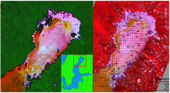
Figure 1. Comparison of sea ice classification results using AVHRR data (left, land masking applied) and SLSTR data (right, no land masking) of 13 April 2018 in northern Bothnian Sea and Bothnian Bay as indicated by the overview map (Refer to Table 2 for colour legend). In the section on the right, the corresponding ice chart by SMHI is overlaid.

Postprocessing was performed by using ocean masking information included in RBT products to set all non-ocean pixels to black colour. Additionally, a cloud mask was formed from spectral channels S3, S7, and S8 as well as a greyscale image showing cloud details which was used to replace the ice classification image at all pixels detected as cloudy.

More than 2500 Sentinel-3 scenes from the years 2017 to 2019 were classified, reprojected to Stereographic or Mercator map projection, and stored in GeoTIFF format. The scenes were selected to cover all suitable seasons and several regions (Baltic Sea Region, Svalbard/East-Greenland, Kara Sea/Franz Joseph Islands, North-West Passage, and Hudson Bay). Figure 2 shows an example of a result computed from SLSTR data collected on 4 May 2019.

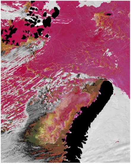
Figure 2. Sea ice classification result based on SLSTR data collected on 4 May 2019 over the area of Franz Joseph Islands to Novaja Semlja. Refer to Table 2 for colour legend.

2.2. Algorithm for Sea Ice Discrimination Using Sentinel-1 SAR Data

A software prototype described in [8] was modified [9] in order to optimally process Sentinel-1 Extended Interferometric Wide Swath (EW) mode data. A Support Vector Machine (SVM) was trained to discriminate three ice classes: “Open Water and Nilas”, “Young Ice”, and “First Year Ice”.

In detail, information from both polarization channels (HH and HV) and grey level co-occurrence matrix based texture parameters are fed into the SVM classifier along with the incidence angle. Readers are referred to Singha 2021 for further details about the algorithm and the training process.

As an example, Figure 3 shows the classification result from a Sentinel-1 acquisition taken on 11 September 2018 over North Greenland. Overall, the algorithm for Sentinel-1 based sea ice classification is able to distinguish the three ice classes “Open Water and Thin Ice”, “Young Ice”, and “First Year Ice” with high reliability, as they yield different radar response properties.

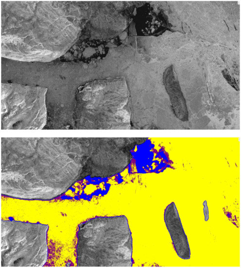
Figure 3. (TOP) Sentinel-1 acquisition (HH) taken on 11th September 2018 over North Greenland (BOTTOM) Corresponding, land masked sea ice classification with blue = Open water and thin ice, violet = young ice, yellow = First Year Ice.

The incidence angle still impairs the classification result. In future work, this problem will be treated by a new method similar to [10].

2.3. Approaches to Combine Sentinel-3 SLSTR and Sentinel-1 SAR Ice Classifications

In the first proposal of a combination, the colour channels of the continuous ice classification based on SLSTR are multiplied at cloud free pixels by SAR based class numbers (0 for background, 1 for blue, 2 for yellow, and 3 for magenta) and the result modulo 256 is saved as a new colour image. In addition, a second method was tried to combine the two ice classification results. As described in detail in Section 3, 19 main colour classes were identified in the SLSTR ice classification results. Based on these main colour classes, the continuous SLSTR ice classification was converted into a form in which only a limited number of different colour classes are represented. Each pair of assignments to classes from SLSTR and SAR then serves as a class in the combination.

In order to assign one of the ice classes to each pixel, a principal component analysis (for details, refer to any book on principal component analysis, e.g. [11]) was carried out. For this purpose, the manually selected test datasets mentioned above were used to estimate the variance covariance matrix of colour components converted to L*a*b* colour space. For each pixel, we compute the difference of the classification colour in L*a*b* colour space to the centre colour of the class in question and transform the result to principal components according to that class. The resulting principal components are expressed in multiples of the standard deviation estimated for that class and component. Then the Euclidean norm of this tuple provides a measure of distance of the pixel to the class. Thus, from this kind of distance, calculated for all classes in question, it is decided, to which class the pixel should be assigned. The three additional classes mentioned above were added as they help avoiding errors.

3. Results

3.1. Verification of the Sentinel-3 SLSTR Ice Classification Results

The SLSTR ice classification results are not only intended to serve as input variables for an algorithm for combined SLSTR-SAR ice classification, but it is also expected that they can be promoted to the user community as a stand-alone product. For this purpose, it is considered necessary to provide a sufficiently detailed legend. Therefore, the authors have subjected the results to careful visual inspection by comparing them with ice maps and other satellite data (Modis, Landsat) and, in some cases, have had them evaluated by an independent expert. As a result, 19 different main colours representing the main distinguishable ice/snow types were thus identified, as summarized in Table 2.

Table 2. Interpretation of main colours appearing in sea ice classification results computed from SLSTR measurements as identified by visual inspection. Mean values of top of atmosphere reflectance in channel S2 and blackbody temperature equivalent to radiation measurements in channel S9 are included for each class as derived from manually selected pixels in various scenes and seasons.

Colour Name and Image of Central Colour in Class	Mean Reflectivity (%) Channel S2	Mean Brightness Temperature (°C) Channel S9	Interpretation
green	4.7	1.3	Open water
green-orange	3.0	−3.2	nearly freezing water, or mixed ice/water pixel or very thin ice (e.g., frazil ice)
bright and dark orange	10.4	−7.5	ice without snow cover; especially dark and light nilas (<10 cm)
medium yellow	28.9	−10.9	young ice without snow cover; especially grey ice (10–15 cm)
light yellow-white	34.8	−11.6	young ice without snow cover; especially grey-white ice (15–30 cm)
dark red	69.7	−20.3	ice of uncertain thickness with dry snow cover
medium red	69.8	−21.6	ice of uncertain thickness with aged dry snow cover
light red	75.5	−24.2	ice of uncertain thickness with aged snow cover
dark pink	80.4	−15.5	ice of uncertain thickness (most likely between 20 and 50 cm) covered by aged snow (increased grain size of snow)
medium pink	82.2	−21.0	ice of uncertain thickness (most likely between 20 and 50 cm) covered by further aged snow compared to dark pink
light pink	83.6	−18.6	ice of uncertain thickness (most likely between 20 and 50 cm) covered by snow
dark violet	84.4	−12.9	ice of uncertain thickness covered by thick, slightly aged snow with very small amount of moisture
light violet	82.1	−11.9	similar to dark violet, but advanced snow metamorphism and moisture
light blue	68.7	−1.2	thick ice covered by slightly wet snow (thickness not well defined)
dark blue	52.3	0.0	Ice covered by increasingly wet snow; partial pixel coverage by meltponds possible
light green	26.5	−2.3	Ice with low snow cover and mainly meltponds, probably refrozen on the surface

For each of the identified classes, a set of test pixels were manually selected from various scenes and for each of these, a set of data was extracted including colour components, reflectivity, and/or blackbody temperature for all SLSTR spectral channels, geometric values such as the sun zenith angle, the satellite viewing zenith angle, and more. These were used to analyse some statistical properties of the classes. Figure 4 presents an overview of the mean reflectivity/blackbody temperature for all SLSTR spectral channels found for the colour classes. The colour sequence from left to right follows the different stages of ice development: on the left the colours during the freezing period, in the middle the colours that occur during increasing aging and on the right the colours that are preferentially seen during melting. Correspondingly, from left to right, the average reflectance values increase as the freezing process progresses and the average brightness temperatures decrease towards the colour class “light red”. The appearance of the blue colourations signals a significant increase in moisture. This is accompanied accordingly by decreasing reflectance values and increasing temperatures from the colour class “Light Blue” to “Dark Blue” and “Light Green”. The latter occurs when the ice is predominantly covered by melt water ponds. Further statistical investigations [12] confirmed these assumptions, as well as verifications using higher-resolution remote sensing data (Landsat-8 and Modis data) and ice maps of the official ice services (see example in Figure 5).

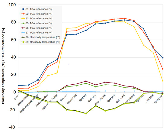
Figure 4. Mean values as measured for top of atmosphere (TOA) reflectance of SLSTR spectral channels S1–S7 and for blackbody temperature equivalent to radiances obtained in channels S8 and S9, for the 16 colours identified as major colours of the SLSTR sea ice classification algorithm. Classes are arranged from left to right in the typical chronology of sea ice formation and decline during an ice season. The determined mean values are connected by line segments to give an impression of intermediate values that occur, e.g., due to mixed pixel contents.

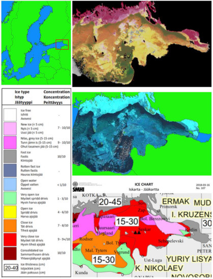
Figure 5. Top left: overview map. Top right: SLSTR sea ice classification in the Gulf of Finland on 16 March 2018. Middle right: Scene collected by Landsat-8 at the same day, partly covering the area of SLSTR classification. Bottom right: Corresponding section of the Swedish ice chart by SMHI and bottom left: ice chart legend.

The new SLSTR-based algorithm automatically calculated consistent results in all cases. As an example, Figure 6 shows a sequence of four products located near the East Greenland coast between 23 and 30 September 2018.

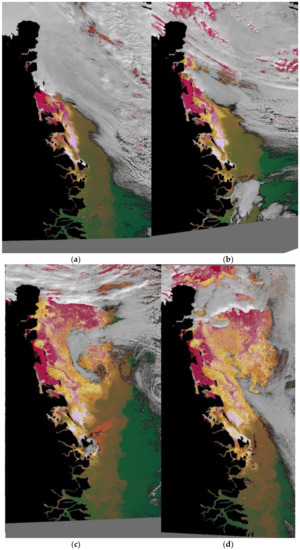
Figure 6. SLSTR ice classification sequence; results of scenes collected along the east coast of Greenland between 70° N and 82° N at 23 (a), 24 (b), 27 (c), and 30 (d) September 2018.

3.2. First Approach to Automatically Combine Sentinel-3 SLSTR and Sentinel-1 SAR Ice Classifications

In the case of the SAR ice class ‘blue’ (open water/nilas/flooded ice), the method described in Section 3.2 results in exactly the same colour as the SLSTR ice classification, while for the other classes new colours are created which contrast well with the old colours. Occasionally, there are points that have closely spaced values in the SLSTR ice classification, but in combination show a transition from 255 to 0 or vice versa in at least one colour channel. Such isolated points were eliminated by applying a median filter. An example of this approach of a potential combination is shown in Figure 7 (12 May 2017, near Franz-Josef-Islands). Under the assumption that correct ice classes are differentiated in each separate ice classification, this type of combination results in five inconsistent combinations. It is, for example, inconsistent, if the SLSTR classification result is ‘open water’ or ‘nilas’ and SAR classification reports ‘ice up to 30 cm’ or ‘ice between 30 cm and 200 cm’. This has to be investigated in a further study. A more detailed analysis of the problem of the mixing pixel for SLSTR could be helpful in these cases. In most cases, however, combinations already clearly show an added value through the application of this method as compared to the individual classifications. Thus, six types of smooth ice (30–200 cm) with aged snow cover can be distinguished as well as four types of young ice up to 30 cm with aged snow cover. In one subarea it has already been possible to identify the surface properties of grey/grey-white ice as smooth first year ice (30–200cm).

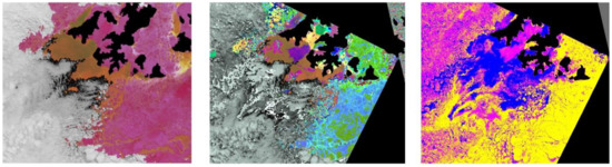
Figure 7. Example of a combination of SLSTR and SAR based ice classification according to first tested algorithm. Data used are collected in the vicinity of Franz Joseph Islands on 12 May 2017. Left: SLSTR ice classification; Right: SAR ice classification; Middle: Combination.

3.3. Second Approach to Combine Sentinel-3 SLSTR and Sentinel-1 SAR Ice Classifications

Although the SLSTR ice classification is a very complex, continuous colour image, which has more variations in colour and colour transitions (ice classes) than the main colour classes mentioned above, e.g., due to mixed pixel contents, the authors decided to generalise the colour classes to a certain extent by assigning each pixel one of the 19 main classes specified in Table 2 and three additional classes, accepting a significant loss of information for visual inspection of the classification results. This generalization, however, leads to a kind of ice map, on which each colour can easily be changed according to customer requirements.

In principle, pixels for which an assignment to one of the three ice classes according to the SAR classification as well as to one of the 19 classes from the SLSTR classification are available, can form a new class in any combination. Thus up to 57 different classes may be formed, but not all of them are useful. Contradictory classes were displayed in white, and the remaining classes and their preliminary colour assignment are listed in Table 3. A special effort was made to ensure that colours representing similar types of ice should be similar and that, overall, the colouring scheme is similar to the colouring in the SLSTR classification. This allows us to include the SLSTR classification at points where no SAR classification is available. Figure 8 presents an example of such a combination. Even if only a few of the theoretically possible classes occur, an additional benefit can be identified and the areas in which SLSTR and SAR classifications contradict each other are clearly visible. When using this method, however, the colouring would have to be coordinated with the user community.

Table 3. Interpretation of main colours appearing in sea ice classification results computed according to the second described approach for SAR—optical ice classification combination.

	SAR Ice Class Colour
SLSTR Ice Class Colour and Ice Class	Colour Used for Combination of SAR Class 1 (Open Water or Nilas up to 10 cm) and SLSTR Class According to Table Row	Colour Used for Combination of SAR Class 2 (Young Ice, 10–30 cm) and SLSTR Class According to Table Row	Colour Used for Combination of SAR Class 3 (Smooth First Year Ice, 30–200 cm) and SLSTR class According to Table Row
open water	open water	open water	inconsistent
freezing ready water	freezing ready water	inconsistent	inconsistent
nilas: 0–10 cm	nilas	nilas	inconsistent
grey ice: 10–15 cm	inconsistent	grey ice up to 15 cm	inconsistent
grey-white ice: 15–30 cm	inconsistent	grey-white ice	smooth grey-white ice near 30 cm
dark red: Ice of unknown thickness covered by dry snow	nilas covered by dry snow	young ice 10–30 cm covered by dry snow	smooth first year ice, 30–200 cm covered by dry snow
medium red: Ice of unknown thickness covered by aged snow	inconsistent	young ice, 10–30 cm covered by aged snow	smooth first year ice, 30–200 cm covered by aged snow
light red; Ice of unknown thickness covered by less aged snow	inconsistent	young ice, 10–30 cm covered by less aged snow	smooth first year ice, 30–200 cm covered by less aged snow
dark pink: Ice covered by aged snow at low temperature	inconsistent	young ice, 10–30 cm covered by aged cold snow	smooth first year ice, 30–200 cm covered by aged cold snow
medium pink: Ice covered by aged snow at low temperature	inconsistent	young ice, 10–30 cm covered by aged cold snow	smooth first year ice, 30–200 cm covered by aged cold snow
light pink: Ice covered by aged snow at low temperature	inconsistent	young ice, 10–30 cm covered by aged cold snow	smooth first year ice, 30–200 cm covered by aged cold snow
dark violet: Ice of uncertain thickness covered by thick, slightly aged snow	inconsistent	young ice, 10–30 cm covered by slightly aged snow	smooth first year ice, 30–200 cm covered by slightly aged snow
light violet: Similar to dark violet, but advanced snow metamorphism	inconsistent	young ice, 10–30 cm covered by aged snow	smooth first year ice, 30–200 cm covered by aged snow
light blue: Thick ice covered by moist snow	nilas covered by moist snow	young ice, 10–30 cm covered by moist snow	smooth first year ice, 30–200 cm covered by moist snow
dark blue: Ice covered by increasingly wet snow; partial cover by meltponds possible	inconsistent	young ice, 10–30 cm covered by increasingly wet snow	smooth first year ice, 30–200 cm covered by increasingly wet snow
light green: Ice with low snow cover and mainly meltponds, probably refrozen on the surface	inconsistent	young ice, 10–30 cm, probably refrozen on the surface	smooth first year ice, 30–200 cm, probably refrozen on the surface
diluting ice (brownish), ice/water mixture	ice/water mixture	ice/water mixture, ice up to 30cm	inconsistent
diluting ice (greenish), ice/water mixture	ice/water mixture	ice/water mixture, ice up to 30cm	inconsistent
light grey-white ice	inconsistent	grey-white ice up to 30 cm, very bright	smooth grey-white ice, at least 30 cm thick

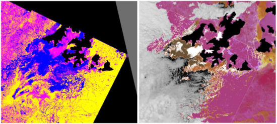
Figure 8. SAR ice classification (left) and combined SAR—optical ice classification computed according to the second described approach (right) for a test case on 12 May 2017 in the vicinity of Franz Joseph Islands.

4. Discussion

4.1. Optical Ice Classification Algorithm Conversion

This work is focused on the SLSTR instrument onboard the Sentinel-3 satellites and the Sentinel-1 SAR instrument. The SLSTR instrument was selected for this first step because of its similarity to the AVHRR instrument, in particular because of its thermal infrared spectral channels and its wide field of view.

At a future stage of product development, it may be appropriate to also include Sentinel-2 data from the MultiSpectral Instrument (MSI) in the processing of the optical ice classification in order to achieve improvements due to the high geometric resolution and probably also due to additional spectral information.

So far, no comparisons have been made with in situ data or observations in the Arctic. Thus, further validation work is needed. However, such data can only be collected selectively, so plausibility studies and personal experience must be relied upon to improve confidence in the algorithm’s ice regime assignments area-wide. Studies of this type are described in the final report of the project [12].

4.2. Optical—SAR Ice Classification Algorithm Combination

An essential goal of the work was to derive and test first fusion concepts for combining the Sentinel-3 and Sentinel-1 based classifications. It is important to note that the time difference of data collection between Sentinel-1 and Sentinel-3 is not too long. It turned out that a time lag of about 3 to 5 h must be expected between SAR and SLSTR scenes. In areas with little ice movement, SLSTR classifications with matching SAR classifications at 200 m resolution could be used for the fusion of both data sets.

After having succeeded in making the NOAA-AVHRR algorithm for ice differentiation usable and automatically applicable to Sentinel-3 SLSTR data, several cases were identified as suitable for comparison to Sentinel-1 SAR data. As an example, scenes taken on 6 and 12 May 2017 over Franz Joseph Land are shown. These scenes have sufficient overlap and were cloudless in some larger areas. The data were transferred geometrically into the same stereographic map projection and resolution.

As a result of the SAR based method of sea ice classification applied to Sentinel-1 SAR data, three classes of sea ice could be detected representing different ice thickness and allowing conclusions on surface roughness:

• open water, or nilas up to 10 cm thick, or flooded ice, displayed in blue;
• young ice: grey ice, or grey-white ice up to 30 cm thick, displayed in yellow;
• ice between 30 cm and 200 cm thick, displayed in magenta.

A manual plausibility check revealed that areas of young ice as well as areas of thick ice can be addressed more precisely by combining them with the Sentinel-3 classification. A good complement, for example, occur in areas of thick ice with snow cover (Sentinel-3) and smooth first year ice (Sentinel-1). Ice floes that are clearly visible in the SAR based ice classification supplemented the Sentinel-3 ice classification, which in some of these areas only indicated extensive ice with dry snow cover. However, areas indicated as open water in the SAR based ice classification suffer from inaccuracies, which will be addressed in future work.

Despite the inconsistencies in those two classifications, the potential of an improved response of the ice types by combining both methods of ice classifications became clear.

In the future, the time delay between SLSTR and SAR scenes will be corrected by using consecutive SLSTR scenes to estimate the conditions at the time of each SAR scene. In general, this is possible because three consecutive scenes are recorded daily at high latitudes under nominal operation—i.e., SLSTR data are provided by two satellites and at an interval on the order of one hour—north of 70° N, and as many as ten or more are recorded north of 77° N, approximately between 3 and 12 h after a morning SAR data collection.

4.3. Further Plans to Improve the Combination of Sentinel-3 SLSTR and Sentinel-1 SAR Ice Classifications

As a better way to generate an ice map from SLSTR and SAR data, the authors recommend supplementing the neural network used to calculate the SAR ice classification by identifying features from the continuous SLSTR classification as additional input. Thus, it can be assumed that in cloudless areas and after additional training, the network is able to significantly improve the recognition of open water areas at the desired spatial resolution. Furthermore, the network can be expected to be much more successful than at present in interpreting the significance of the SAR parameters as a function of surface moisture in terms of ice classes.

5. Conclusions

This paper presents the results of a first step towards a new combined product for sea ice classification generated from Sentinel-3 SLSTR and Sentinel-1 SAR data suitable for providing shipping support in Arctic and subarctic ocean waters. The work consists of:

• adapting and improving a sea ice classification based on NOAA AVHRR to work with Sentinel-3 SLSTR data;
• verifying the SLSTR based algorithm by expert’s visual inspection, comparison to ice maps available, as well as higher resolution satellite images adapting a sea ice classification algorithm based on RADARSAT2 or TerraSAR-X SAR data to work with Sentinel-1 SAR data;
• demonstrating that additional information is gained even by applying simple approaches to combine the results of two algorithms mentioned above;
• proposing a neural network for a more sophisticated combination to be investigated in future.

The investigations will be continued by implementing the outlined combination approach and optimizing it for operational use. The results will be used to establish a processing chain involving additional partners and test users, who will evaluate the advantage for ice detection, contribute to the design of the final products, and take over the later provision of the products on board ships.

References

- Dey, B. Applications of Satellite Thermal Infrared Images for Monitoring North Water during the Periods of Polar Darkness. J. Glaciol. 1980, 25, 425–438. [Google Scholar] [CrossRef][Green Version]
- Aguirre, M.; Berruti, B.; Bezy, J.; Drinkwater, M.; Heliere, F.; Klein, U.; Mavrocordatos, C.; Silvestrin, P.; Greco, B.; Benveniste, J. Sentinel-3—The Ocean and Medium-Resolution Land Mission for GMES Operational Services. ESA Bull. 2007, 131, 29. [Google Scholar]
- Donlon, C.; Berruti, B.; Buongiorno, A.; Ferreira, M.-H.; Féménias, P.; Frerick, J.; Goryl, P.; Klein, U.; Laur, H.; Mavrocordatos, C.; et al. The Global Monitoring for Environment and Security (GMES) Sentinel-3 mission. Remote Sens. Environ. 2012, 120, 37–57. [Google Scholar] [CrossRef]
- Riggs, A.G.; Hall, D.K.; Ackerman, A.S. Sea Ice Extent and Classification Mapping with the Moderate Resolution Imaging Spectroradiometer Airborne Simulator. Remote Sens. Environ. 1999, 68, 152–163. [Google Scholar] [CrossRef]
- König, C. Eisfernerkundung mit NOAA-AVHRR und SAR. Dtsch. Hydrogr. Z. 1995, 4. ISSN 0946-2015. Available online: https://openlibrary.org/books/OL76781M/Eisfernerkundung_mit_NOAA-advanced_very_high_resolution_radiometer_%28AVHRR%29_und_synthetic_aperture_ra (accessed on 23 November 2021).
- Kidwell, K. (Ed.) NOAA Polar Orbiter Data User’s Guide (TIROS-N, NOAA-6, NOAA-7, NOAA-8, NOAA-9, NOAA-10, NOAA-11, NOAA-12, NOAA-13 and NOAA-14). NOAA NESDIS, November 1998. Available online: https://web.archive.org/web/20161209021928/https://www.ncdc.noaa.gov/oa/pod-guide/ncdc/docs/podug/index.htm (accessed on 23 November 2021).
- Robel, J.; Graumann, A. (Eds.) NOAA KLM Users’s Guide with NOAA-N, N Prime, and MetOp Supplements. NOAA NESDIS, April 2014. p. 2530. Available online: https://www.star.nesdis.noaa.gov/mirs/documents/0.0_NOAA_KLM_Users_Guide.pdf (accessed on 23 November 2021).
- Ressel, R.; Frost, A.; Lehner, S. A Neural Network-Based Classification for Sea Ice Types on X-Band SAR Images. IEEE J. Sel. Top. Appl. Earth Obs. Remote Sens. 2015, 8, 3672–3680. [Google Scholar] [CrossRef]
- Singha, S. Towards Pan-Arctic Sea Ice Type Retrieval Using Sentinel-1 TOPSAR Modes. In Proceedings of the EUSAR 2021—13th European Conference on Synthetic Aperture Radar, Online Event, 29 March–1 April 2021; Available online: https://www.vde-verlag.de/proceedings-de/455457180.html (accessed on 23 November 2021).
- Park, J.-W.; Korosov, A.A.; Babiker, M.; Sandven, S.; Won, J.-S. Efficient Thermal Noise Removal for Sentinel-1 TOPSAR Cross-Polarization Channel. IEEE Trans. Geosci. Remote Sens. 2017, 56, 1555–1565. [Google Scholar] [CrossRef]
- Jolliffe, I. Principal Component Analysis, 2nd ed.; Springer: New York, NY, USA, 2002; Available online: http://cda.psych.uiuc.edu/statistical_learning_course/Jolliffe%20I.%20Principal%20Component%20Analysis%20(2ed.,%20Springer,%202002)(518s)_MVsa_.pdf (accessed on 23 November 2021).
- König, C.; König, T.; Frost, A.; Jacobsen, S. Verbesserung der Meereis-Lageinformationen für die Schifffahrt in Polaren Gewässern Durch Kombinierte Meereis-Klassifikation mit optischen Daten der Sentinel-3 und SAR-Daten der Sentinel-1 Satellitenserie." Final Report of Project EisKlass31 (in German), Project Timeframe: August 2018—July 2019, Submitted to: Technische Informationsbibliothek Hannover. 2019. Available online: https://www.tib.eu/de/suchen/id/TIBKAT:1767649789/Verbesserung-der-Meereis-Lageinformationen-f%C3%BCr?cHash=2af0a7aa5ec710dffa6a7553d8a8a58f (accessed on 23 November 2021).
Publisher’s Note: MDPI stays neutral with regard to jurisdictional claims in published maps and institutional affiliations. |
© 2021 by the authors. Licensee MDPI, Basel, Switzerland. This article is an open access article distributed under the terms and conditions of the Creative Commons Attribution (CC BY) license (https://creativecommons.org/licenses/by/4.0/).