Daily Flood Monitoring Based on Spaceborne GNSS-R Data: A Case Study on Henan, China

Abstract

Flood is a kind of natural disaster that is extremely harmful and occurs frequently. To reduce losses caused by the hazards, it is urgent to monitor the disaster area timely and carry out rescue operations efficiently. However, conventional space observers cannot achieve sufficient spatiotemporal resolution. As spaceborne GNSS-R technique can observe the Earth’s surface with high temporal and spatial resolutions; and it is expected to provide a new solution to the problem of flood hazards. During 19–21 July 2021, Henan province, China, suffered a catastrophic flood and urban waterlogging. In order to test the feasibility of flood disaster monitoring on a daily basis by using GNSS-R observations, the CYGNSS (Cyclone Global Navigation Satellite System) Level 1 Science Data were processed for a few days before and after the flood to obtain surface reflectivity by correcting the analog power. Afterwards, the flood was monitored and mapped daily based on the analysis of changes in surface reflectivity from spaceborne GNSS-R mission. The results were evaluated based on the image from MODIS (Moderate Resolution Imaging Spectroradiometer) data, and compared with the observations of SMAP (Soil Moisture Active Passive) in the same period. The results show that the area with high CYGNSS reflectivity corresponds to the flooded area monitored by MODIS, and it is also in high agreement with SMAP. Moreover, CYGNSS can achieve more detailed mapping and quantification of the inundated area and the duration of the flood, respectively, in line with the specific situation of the flood. Thus, spaceborne GNSS-R technology can be used as a method to monitor floods with high temporal resolution.

1. Introduction

Floods are one of the most common and destructive natural disasters in the world. The occurrence of floods has a severe impact on human life and the environment. And it causes severe economic losses to society [1,2,3]. Climate factors and geographical environment are essential reasons behind flooding. After heavy rains, when water overflows lakes and dams, floods occur in low-lying areas. In case of high-intensity, large-scale rainstorms, the affected area is prone to flooding and serious disasters that may even inundate the cities [4,5]. Recently, Zhengzhou, Henan Province and other cities have encountered extreme weather, which has caused serious floods. Timely and detailed mapping of the inundated area and also the disaster-affected area is essential for post-disaster rescue and restoration. Additionally, it can help relevant departments better understand the temporal and spatial evolution of this type of disaster, and provide references for the areas that may be affected again [6,7].

At present, flood monitoring on a large scale can be achieved using spaceborne remote sensing data. Optical remote sensing systems (for example, MODIS, Sentinel-2) can provide data with good spatial resolution [8,9]. However, they cannot penetrate clouds and Earth’s surface is usually obscured by clouds during floods. Therefore, they are often unable to monitor the progress of floods. Microwave remote sensing, in contrast, is not affected by these limitations. However, current active radar satellites cannot provide observations with high spatial and temporal resolution at the same time. For example, Synthetic Aperture Radar (SAR) can provide observations with high spatial resolution, but the revisit period is long (6–11 days, e.g., TerraSAR-X, and Sentinel-1 SAR) [10]. Due to the high dynamics of floods, SAR images cannot be used to monitor floods.

GNSS-R (Global Navigation Satellite System -Reflectometry) technology is a remote sensing technology that extracts geophysical parameters by receiving and processing GNSS signals reflected on the Earth’s surface [11]. This technology is an effective microwave remote sensing method, and it has numerous GNSS signals (e.g. GPS, Galileo, GLONASS, and BDS) as a source of opportunity [12]. A constellation of GNSS-R small satellites can provide a much shorter revisit time, and NASA launched a CYGNSS (Cyclone Global Navigation Satellite System) satellite constellation in December 2016, which provides sufficient data to facilitate the use of GNSS-R technology. The overall median revisit time is 2.8 h, and the mean revisit time is 7 h [13]. Theoretically, the reflected footprint of CYGNSS is nearly 0.5 km × 0.5 km. For oceans with very rough surfaces, the spatial resolution is approximately 25 km × 25 km [14]. CYGNSS uses a passive sensor with L-band frequency waves and can work irrespective of time or weather conditions [15]. Thus, compared with other remote sensing technologies (such as optical and active remote sensing varieties), CYGNSS observations for flood monitoring can meet the requirements of high dynamics. At present, spaceborne GNSS-R data are being used to conduct research on sea ice and sea altimetry [16,17,18], soil moisture [19,20,21], sea surface wind speed [22,23], flood monitoring [24,25], surface vegetation water content [26] etc. The papers [15,21] indicate that the reflectivity obtained from TDS-1 and CYGNSS data can be used to perceive surface water bodies, such as lakes and rivers. The reflectivity of water bodies is higher and that of arid areas is lower. This mechanism can help detect soil moisture, flooding areas and inland waters.

This paper uses CYGNSS high temporal and spatial resolution data for flood monitoring. The main content is to quantify the occurrence and duration of flood caused by extreme weather in Henan, and to map the distribution of the inundated area and those most affected by the flood. Additionally, SMAP monitoring results and optical remote sensing images can be used for comparison and verification of data obtained from the former. The methodology for processing data is the same as those used described by the authors of [21,25].

2. Materials and Methods

2.1. CYGNSS Data

2.1.1. CYGNSS Mission

CYGNSS is a NASA Earth Venture mission consisting of eight small satellites that receive direct and reflected signals from GPS satellites. CYGNSS is designed to observe the wind speed on the ocean surface during a hurricane and, therefore, it scans the tropical orbit at an inclination of 35 degrees, covering only 38° South latitude to 38° North latitude, and its receiver and software are optimized for ocean surface remote sensing [27]. Each CYGNSS satellite carries two downward antennas and a GNSS-R receiver, which can simultaneously provide GNSS-R observations from four different GPS satellites. CYGNSS has announced marine and terrestrial products, and has provided free data access and download services since March 2017 at https://podaac-opendap.jpl.nasa.gov, (accessed on 30 July 2021). CYGNSS data products are divided into three levels. The Level 1 (L1) dataset contains surface bistatic radar cross section (BRCS) measurements; the Level 2 (L2) dataset includes derived spatial average wind speed and mean square slope (MSS); and the Level 3 (L3) dataset is gridded wind speed. The product has a time resolution of 1 h and a spatial resolution of 0.2° × 0.2°. Since the data interval of CYGNSS is 1 s, 32 sets of measurements can be obtained simultaneously per second. And the CYGNSS constellation composed of eight small satellites can provide a relatively short revisit time so that it can provide observations with high temporal and spatial resolution.

This paper uses CYGNSS Level 1 ScienceData products (Version 3.0.), and the data period is from 19 July to 27 July 2021. Compared with the previous data (Version 2.1.), this version re-estimates GPS EIRP (Effective Isotropic Radiated Power) by using direct signal power and antenna gain assessed by the CYGNSS time delay doppler measuring instrument [28].

2.1.2. CYGNSS SR

The configuration function of the CYGNSS and GPS constellation can be regarded as the L-band bistatic radar. The CYGNSS receiver receives the forward-scattered circularly polarized signal from the Earth’s surface transmitted by the GPS satellite, and obtains the characteristics of and information on the surface below (ocean or land). The inland water bodies are also part of the land information obtained from the bistatic radar. Thus, we first obtain the surface reflectivity (SR) through the bistatic radar equation [29] to further complete flood monitoring.

The main product parameter of CYGNSS is a delay-Doppler map, referred to as DDM [30]. DDM consists of two parts: coherent and incoherent components [31]. Assuming that CYGNSS land observations are mainly specular reflection points, that is, the surface is relatively smooth, and the reflected signals are coherent and come from the area defined by the first Fresnel zone, the coherent component of DDM can be expressed as [32,33]:

$${ \mathrm{P}}_{\mathrm{RL}}^{\mathrm{coh}}=\frac{{\mathrm{P}}_{\mathrm{r}}^{\mathrm{t}}{\mathrm{G}}^{\mathrm{t}}}{{4\mathsf{\pi }(\mathrm{R}}_{\mathrm{ts}}{+\mathrm{R}}_{\mathrm{sr}}{)}^2}\frac{{\mathrm{G}}^{\mathrm{r}}{\mathsf{\lambda }}^2}{4\mathsf{\pi }}{Г}_{\mathrm{RL}}$$

(1)

And Table 1 shows the details of the equation.

Table 1. The implication of each variable in Equation (1).

Variables	Implication
${\mathrm{P}}_{\mathrm{r}}^{\mathrm{t}}$	transmitted RHCP power
${\mathrm{G}}^{\mathrm{t}}$	gain of the transmitting antenna
${\mathrm{G}}^{\mathrm{r}}$	gain of the receiving antenna
${\mathrm{R}}_{\mathrm{ts}}$	distance between the transmitter and the specular point
${\mathrm{R}}_{\mathrm{sr}}$	distance between the specular reflection point and the receiver
λ	GPS wavelength
${Г}_{\mathrm{RL}}$	surface reflectivity

What we actually obtain is surface reflectivity and thus all terms in the Equation (1) are converted into dB form, as in Equation (2) [24]:

$${Г}_{\mathrm{RL}}{\left[\mathrm{dB}\right]=10\mathrm{logP}}_{\mathrm{RL}}^{\mathrm{coh}}-10\log {\mathrm{P}}_{\mathrm{r}}^{\mathrm{t}}-10\log {\mathrm{G}}^{\mathrm{t}}-10\log {\mathrm{G}}^{\mathrm{r}}+20\log ({\mathrm{R}}_{\mathrm{ts}}{+\mathrm{R}}_{\mathrm{sr}})+20\log 4\mathsf{\pi }-20\log \mathsf{\lambda }$$

(2)

Table 2 is the CYGNSS dataset parameters used in Equation (2).

Table 2. The variables in Equation (2) and the corresponding CYGNSS dataset parameters.

Variables	CYGNSS Parameters
${\mathrm{P}}_{\mathrm{r}}^{\mathrm{t}}{\mathrm{G}}^{\mathrm{t}}$	gps_eirp
${\mathbf{G}}^{\mathbf{r}}$	sp_rx_gain
${\mathrm{R}}_{\mathrm{ts}}$	tx_to_sp_range
${\mathrm{R}}_{\mathrm{sr}}$	rx_to_sp_range

The peak value of ‘ddm_snr’ or ‘power_analogue’ can be used instead of ${\mathrm{P}}_{\mathrm{RL}}^{\mathrm{coh} }$ [15,21]. In this paper, the peak value of ‘power_analogue’ is used to calculate surface reflectivity.

2.1.3. Quality Control

Through Equation (2), we obtain the CYGNSS reflectivity. In order to better apply CYGNSS data to flood monitoring, several corrections are performed to control the quality of the data. Firstly, CYGNSS reflectivity is a left-handed circular polarization reflectivity which is related to incidence angles [19]. Based on the soil moisture work of Chew et al. in 2020, we removed the observations with incidence angles greater than 65°. In addition, we do not consider the observations that the signal-to-noise ratio is less than 2 dB and the receiver antenna gain is less than 5 dB [21].

2.2. SMAP Data

The comparison product used in this paper comes from the SMAP satellite. The SMAP satellite mission was launched by NASA in January 2015. The SMAP satellite is equipped with active radar and passive radiometer sensors, and its revisit period is 2–3 days. By measuring brightness as well as temperature and performing geophysical inversion to obtain global soil moisture information, it can provide users with global soil moisture estimates [34].

The observations of SMAP are mainly divided into data collected by passive L-band radiometer and those gathered by active L-band radar. The GPS L1 frequency band is approximately 1.58 GHz and the operating frequency of the SMAP radiometer is approximately 1.41 GHz. These two types of data have similar frequencies and sensitivity to the land surface [35], and therefore, SMAP data are used for analysis and comparison with CYGNSS data.

SMAP products use EASE-grid 2.0 to record data. The active radar fails after two months in orbit, and the spatial resolution of the microwave radiometer measurement data is approximately 40 km. Thus, the SMAP L3 Radiometer Global Daily 36 km EASE-Grid Soil Moisture (Version 7) product is used in this paper. The data period is from 1 July to 15 August 2020.

2.3. Study Area

Henan is located in central China. The province is bounded by latitude 31°23′–36°22′ north, longitude 110°21′–116°39′ east, bordering Anhui and Shandong in the east, Hebei and Shanxi in the north, Shaanxi in the west and Hubei in the south, a total area of 167,000 square kilometers. The terrain of Henan Province is high in the west and low in the east. It is composed of plains and basins, mountains, hills, and water surfaces. Most of them are located in the warm temperate area; and the south spans the subtropical area. The province has a continental monsoon climate with a transition from the northern subtropical area to the warm temperate area.

Henan is on the verge of subtropical high in mid-July. The abundant water vapor in the atmosphere undergoes continuous and intense vertical ascension and turns into raindrops when it is cold, thus producing torrential rain. The Henan catastrophic flood disaster was caused by torrential rain. On 18 July 2021, Typhoon No. 6 ‘Fireworks’ formed in the western Pacific region and approached China. A large amount of water vapor was transported from the sea to the inland of China under the guidance of the typhoon’s peripheral and easterly airflow on the south side of the subtropical high pressure, which provided the rainfall in Henan. The entry of such warm air provides a constant and abundant source of water vapor. At the same time, the atmospheric circulation situation remains relatively stable. In mid-July, the western Pacific subtropical high and the continental high remain stable in the Sea of Japan and Northwest China, respectively. As a result, the low-pressure weather system between the two is stagnant and moves less into the Huanghuai area. The low-pressure weather system is conducive to the vertical upward movement of the atmosphere to produce precipitation. In addition, the particular topography of the Taihang and Funiu mountains in Henan Province has a convergent effect on the easterly airflow that transports water vapor, which makes the vertical ascent more intense and the rainfall stronger.

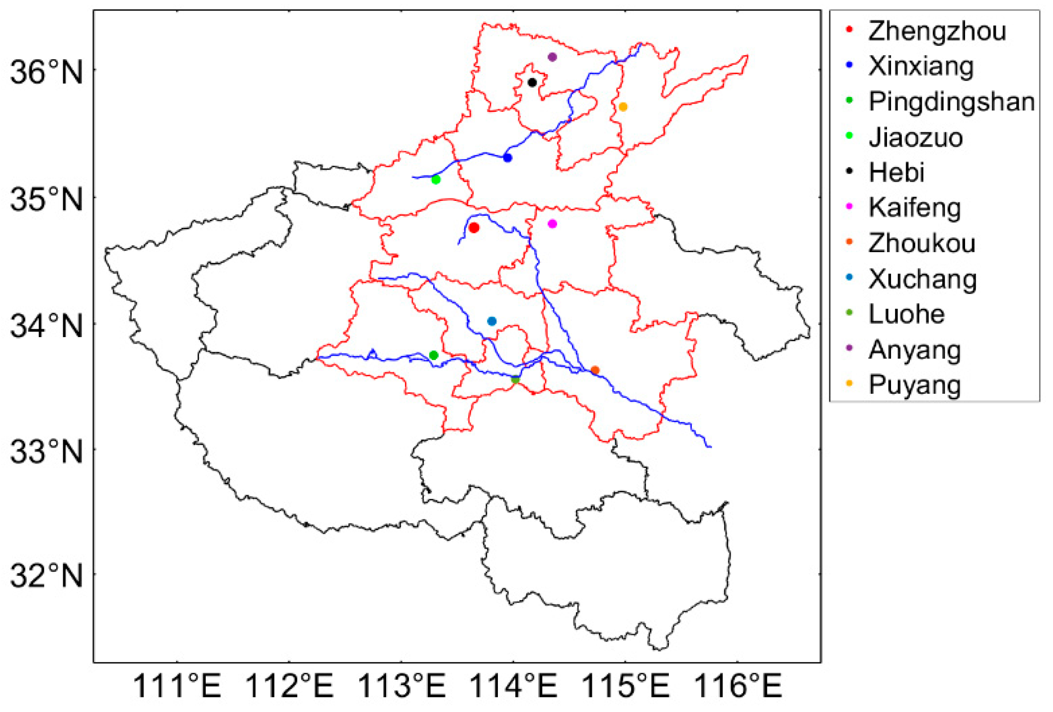
Figure 1 is a map of Henan Province, including 17 prefecture-level cities and one provincial-level municipality. The cities affected by the flood are marked.

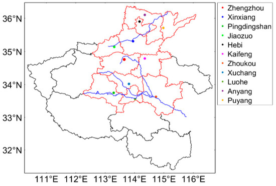
Figure 1. The red areas are the main 11 cities affected by the Henan flood, of which Xinxiang (blue dot) and Zhengzhou (red dot) are the most severely affected areas. From top to bottom, the blue jagged lines represent Wei River, Jialu River, Ying River, and Sha River.

2.4. Remote Sensing Images

MODIS (Moderate Resolution Imaging Spectroradiometer) is a vital instrument on Terra (initally called EOS AM-1) and Aqua (initally called EOS PM-1) satellites. Terra’s orbit around the earth is fixed so that it crosses the equator from north to south in the morning, and Aqua crosses the equator from south to north in the afternoon. Terra MODIS and Aqua MODIS acquire data in 36 spectral bands by observing the entire Earth’s surface every 1 to 2 days, covering the visible to infrared bands. These data help us study and understand the global dynamics and processes in the ocean, the lower atmosphere, and land. MODIS plays an essential role in the development of earth system models that can accurately predict global changes, and can help decision-makers take relevant measures to protect our environment.

Figure 2 is a false-color image of northern Henan Province on 26 July 2021 acquired from the Moderate Resolution Imaging Spectrometer (MODIS) on NASA’s Aqua satellite (https://modis.gsfc.nasa.gov, accessed on 30 July 2021).

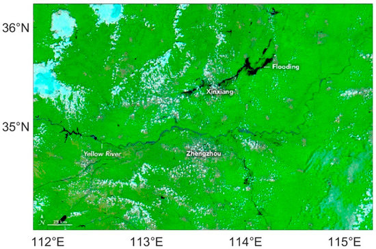
Figure 2. MODIS images in northern Henan after the flood (on 26 July 2021). In this type of image, the vegetation is bright green and the water is dark blue.

It can be seen from Figure 2 that the flooding caused by heavy rain in mid-July 2021 is still visible.

3. Results

3.1. CYGNSS Observations

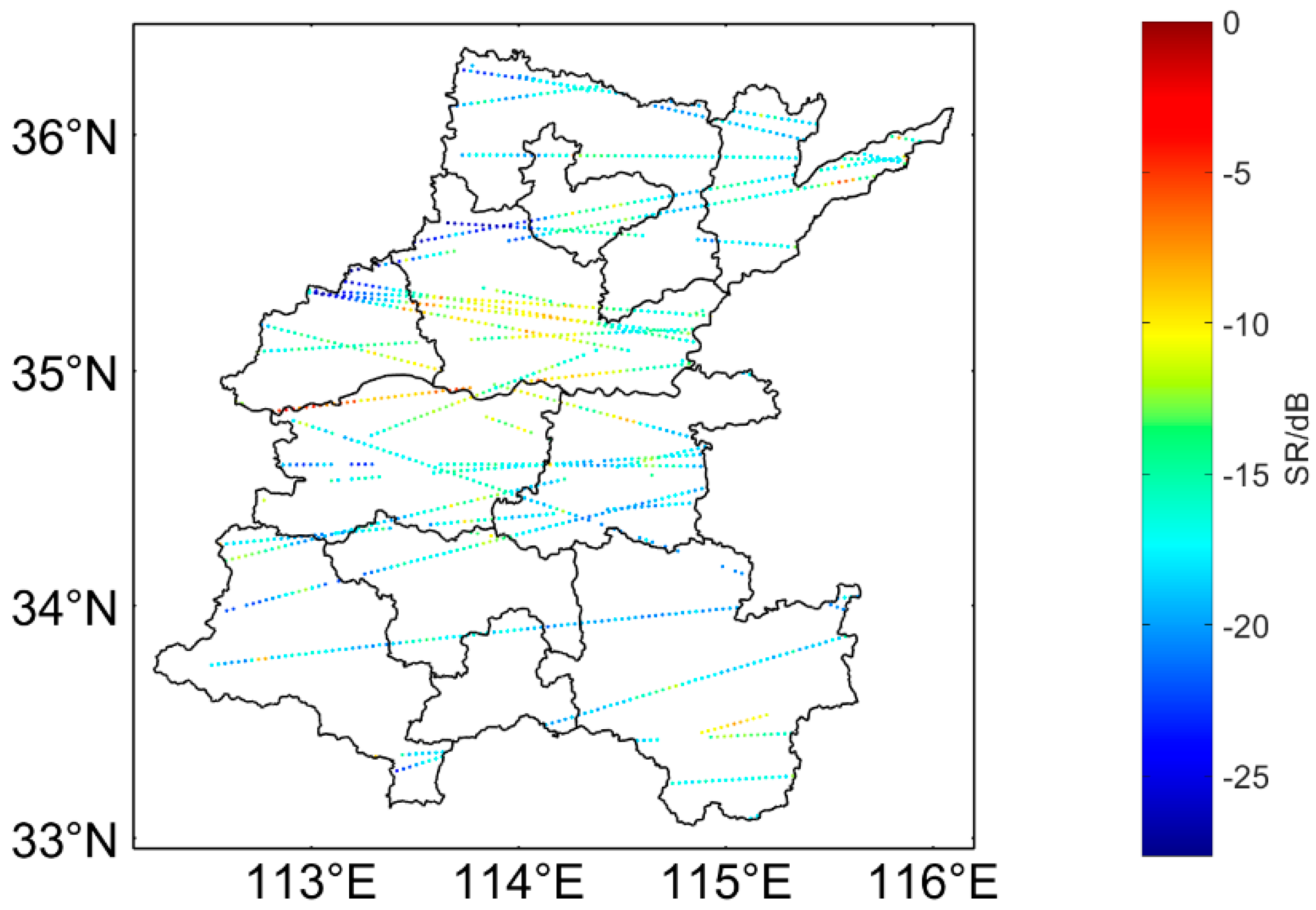
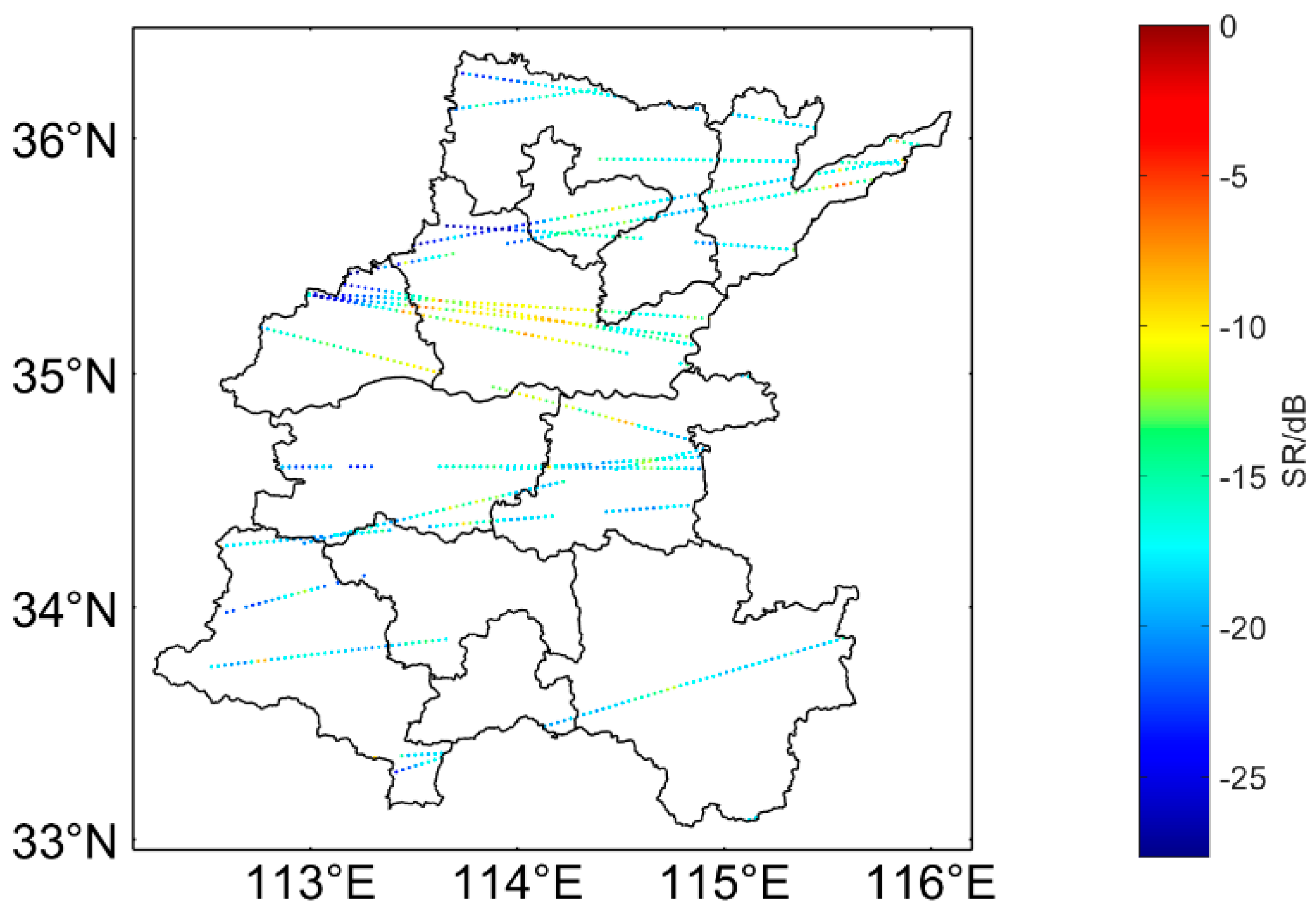
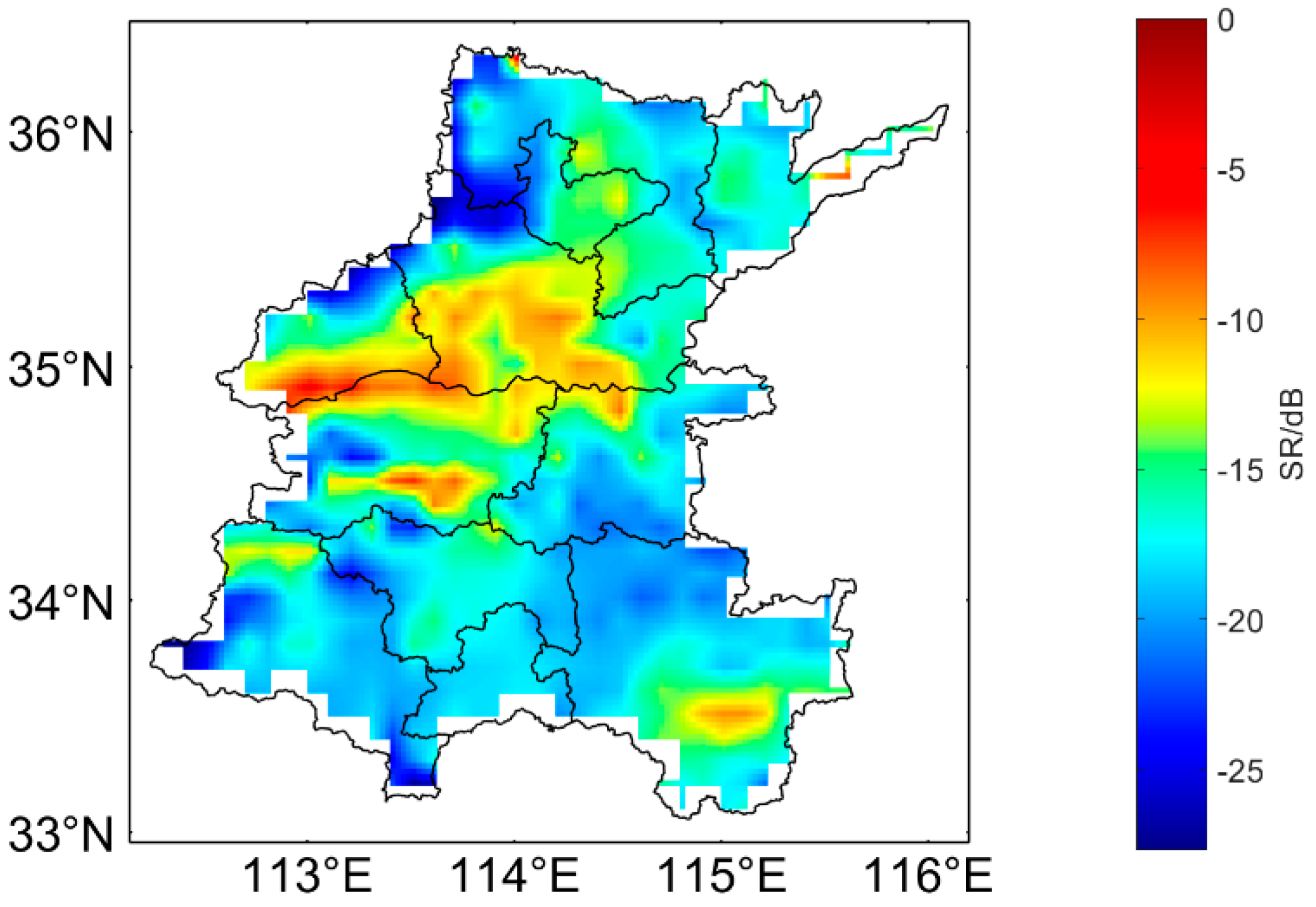
Figure 3 shows the CYGNSS SR measurements in the main affected cities in Henan from 20 July 2021. Figure 4 shows the CYGNSS measurements after quality control obtained through Section 2.1.2. The data are the points sampled by CYGNSS along the satellite tracks. And for the CYGNSS data for our study area, we generated a grid (approximately 3 × 3 square kilometers) and applied linear interpolation. Figure 5 shows the gridded data. As can be seen from the figure, the gridded data are more sensible than satellite tracks representation.

Figure 3. CYGNSS sampling points along the satellite tracks on 20 July 2021.

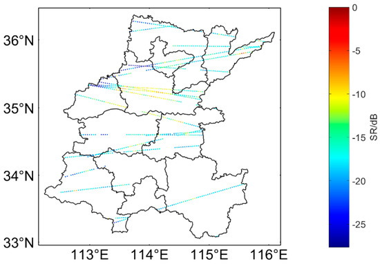
Figure 4. CYGNSS sampling points after quality controls on 20 July 2021.

Figure 5. The results of interpolation processing for SR after quality control on 20 July 2021.

3.2. The Occurrence and the Duration of the Flood

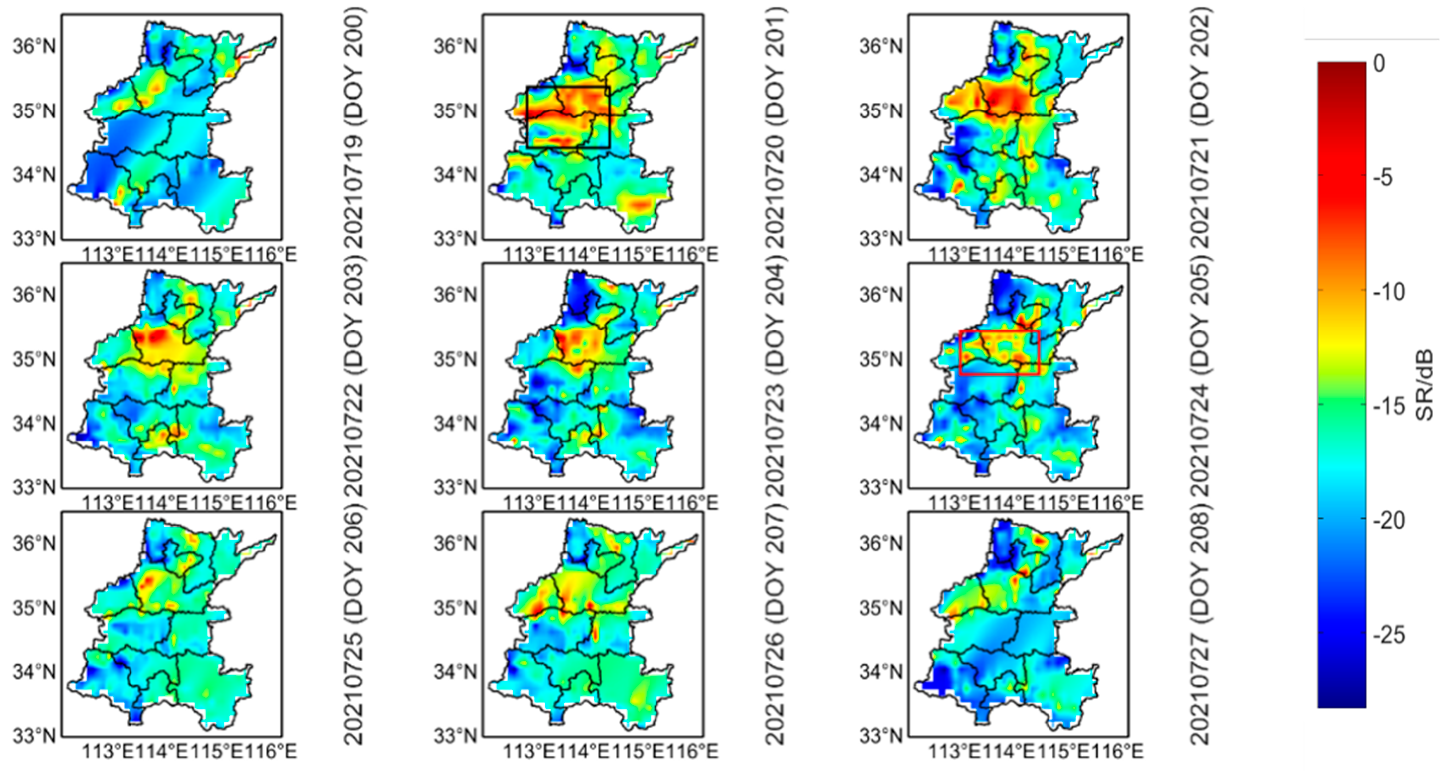
Since CYGNSS reflectivity is sensitive to water bodies, we generated a temporal map of the CYNGSS reflectivity to show the evolution of the flood. As shown in Figure 6, the changes of daily CYGNSS reflectivity are mapped to monitor flood changes (from 19 July to 27 July 2021).

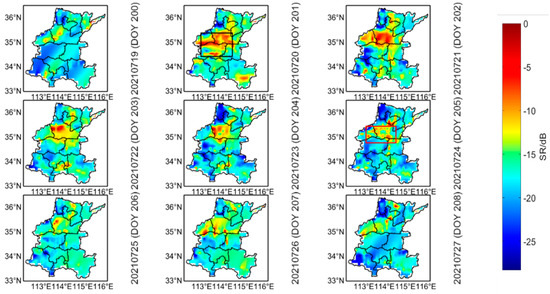
Figure 6. Using CYGNSS SR to monitor floods (from 19 July to 27 July 2021, one day as a period).

It can be seen that the CYGNSS reflectivity (black box) began to increase, which means that the flood occurred on 20 July 2021. And the CYGNSS reflectivity (red box) maintained until 24 July 2021. This shows that the flood duration is about 5 days (from 20 July to 24 July 2021). The flood began to fade away gradually on 25 July 2021.

3.3. The Inundated Areas of the Flood

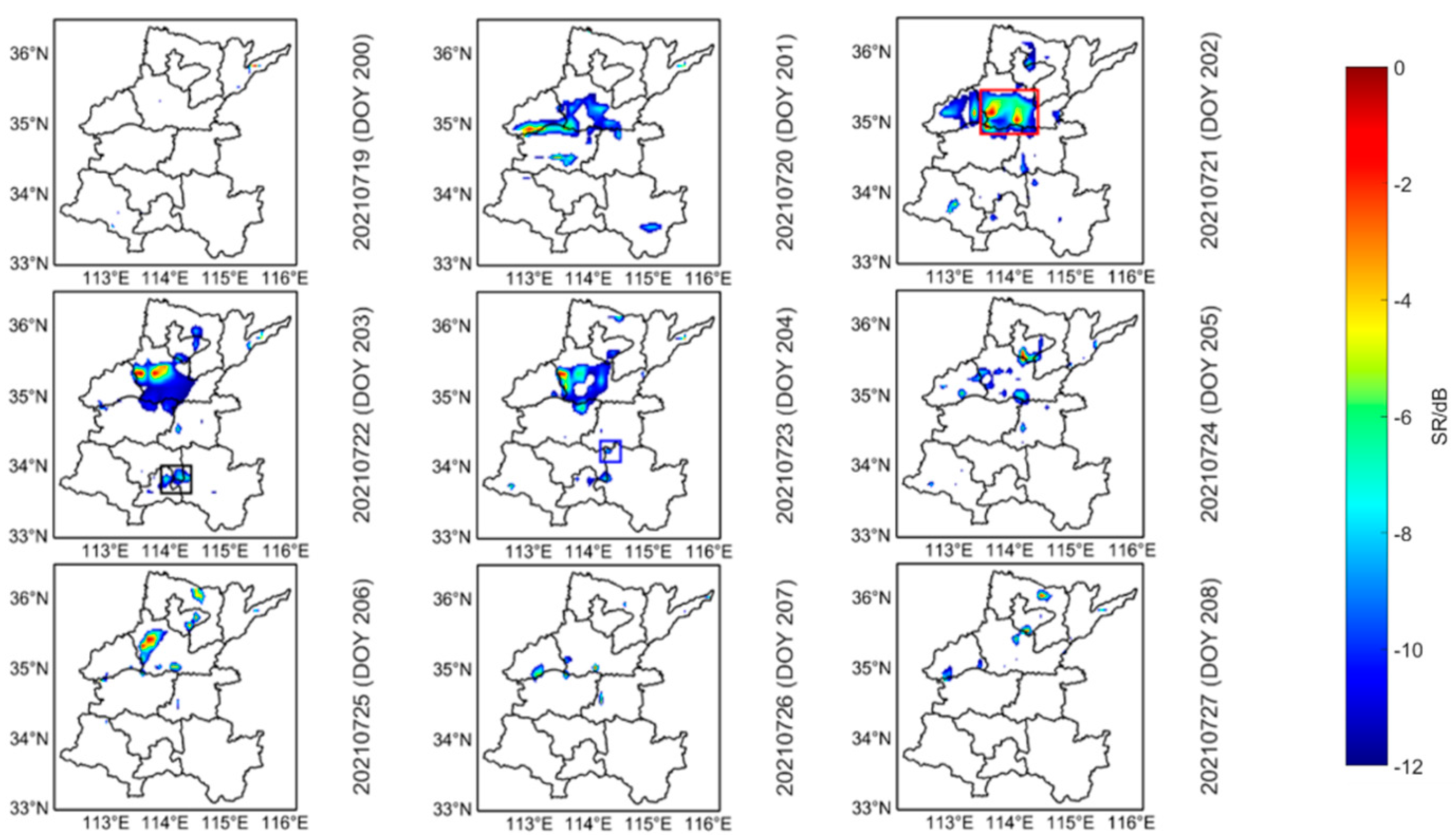
In order to calculate the inundated areas of the flood, the same method [24,25] was used in this study to distinguish inundated areas from the non-inundated areas. We used the CYGNSS reflectivity in permanent water for one year and the median of these observations was used as the threshold between the water and the land. Considering the attenuation of CYGNSS reflectivity caused by the terrain (plains etc.) and vegetation (farmland etc.) coverage in Henan, the difference from [24,25] is that this paper tries to set the threshold to −12 dB. As is seen in Figure 7, observations greater than −12 dB correspond to the flooded areas from 19 July to 27 July 2021 (a period consisting of one day). Figure 7 also shows the distribution of the areas most affected by the flood.

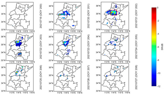
Figure 7. Using CYGNSS SR to monitor the changes in the inundated areas (a period of one day from 19 July to 27 July 2021).

As shown in Figure 7, on 20 July 2021, the flood concentrated in Zhengzhou and southern Xinxiang. On 21 July 2021, the areas most affected by the flood were located in Xinxiang (red box). On 22 July 2021, floods in Pingdingshan, Luohe and Xuchang were discharged through the Ying River into the Sha River, and the areas most affected by the flood were located in the western region of Zhoukou (black box). On 23 July 2021, it was found that floods in Zhengzhou would be discharged through the Jialu River and would reach the northern flood discharge area of Zhoukou (blue box). On 24 July 2021, the inundated area gradually reduced and the flood began to recede leaving only some areas of Xinxiang most affected by the flood.

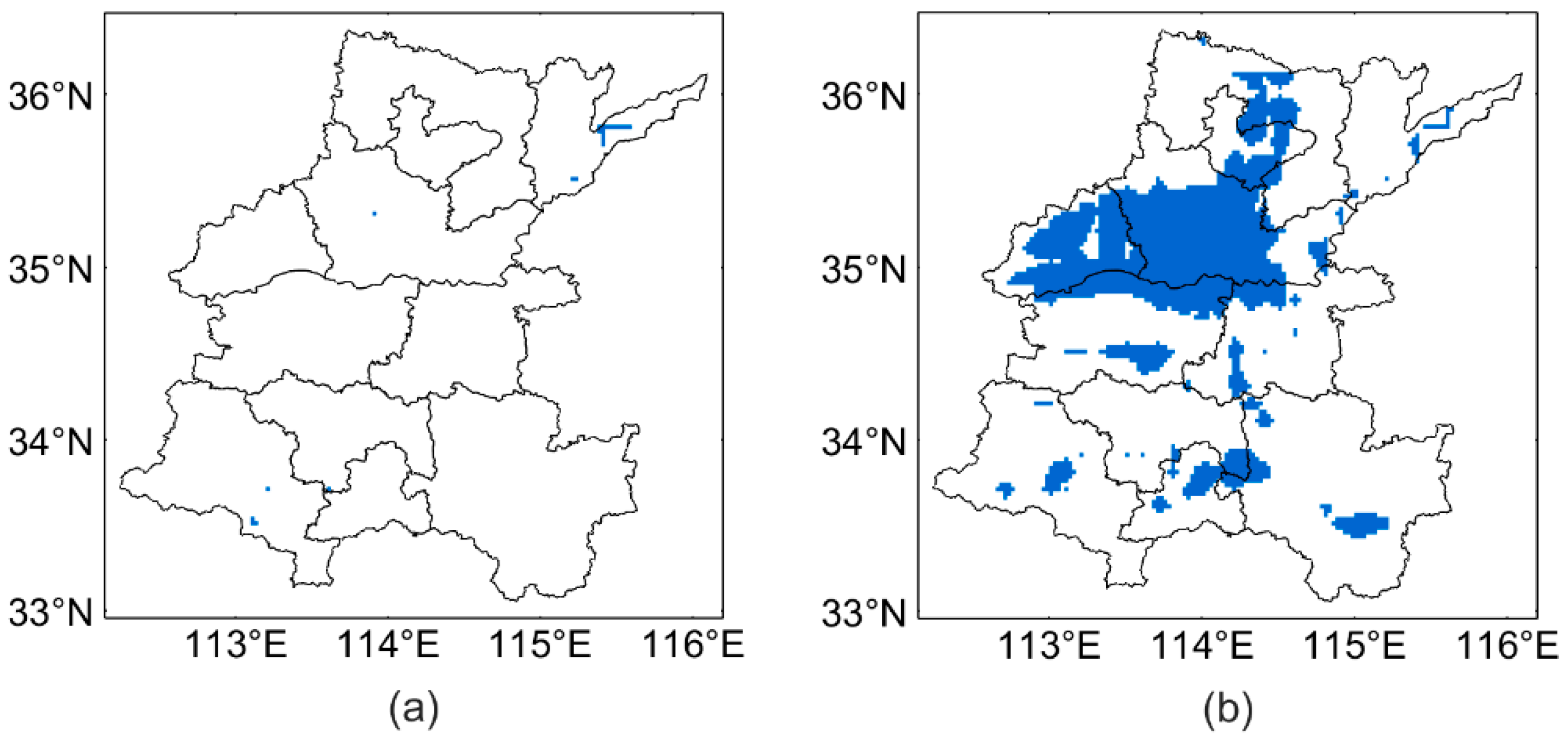
Finally, we mapped the inundated area before and after the flood, as shown in Figure 8.

Figure 8. A threshold was used to distinguish between the inundated and non-inundated areas. (a)The non-inundated area before the flood (on 19 July 2021). (b) The inundated area after the flood (summarized data from 20 July to 24 July 2021).

Table 3 shows the inundation area of the affected cities from 20 July to 24 July 2021.

Table 3. The inundation area of the affected cities.

City	Inundated Area (Square Kilometers)
Xinxiang	6532
Jiaozuo	3270
Zhengzhou	2505
Anyang	1200
Zhoukou	1170
Hebi	998
Kaifeng	893
Luohe	495
Pingdingshan	420
Xuchang	330
Puyang	90

Compared to the situation before the flood, the inundated area in Henan increased by approximately 17,903 square kilometers, of which Xinxiang was found to be the most affected.

3.4. SMAP Monitoring Results

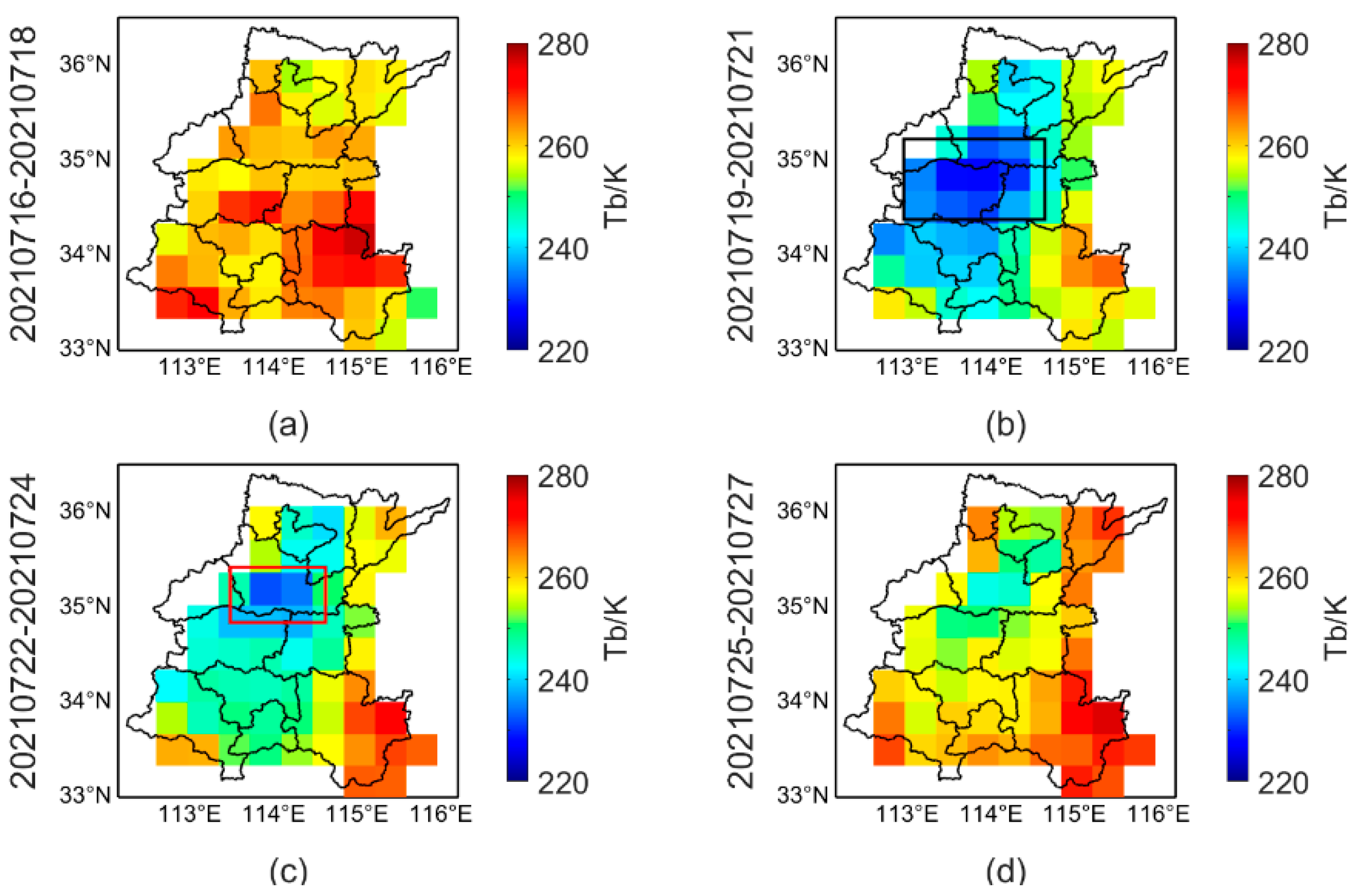
Firstly, we use the brightness temperature (Tb) and soil moisture observed by SMAP microwave radiometer to monitor the flood. Since GNSS signals are circularly polarized, it is necessary to convert the linearly polarized Tb measured by SMAP into circularly polarized Tb [25,36]. Then, the changes in brightness temperature and soil moisture were used to reflect the impact of flooding. As shown in Figure 9 and Figure 10, we mapped the SMAP brightness temperature and soil moisture over a period of three days from 16 July to 27 July 2021 (close to the temporal resolution of SMAP data), and monitored the flood.

Figure 9. (a–d) are the changes in the brightness temperature obtained from SMAP before and after the flood (from 16 July to 27 July 2021).

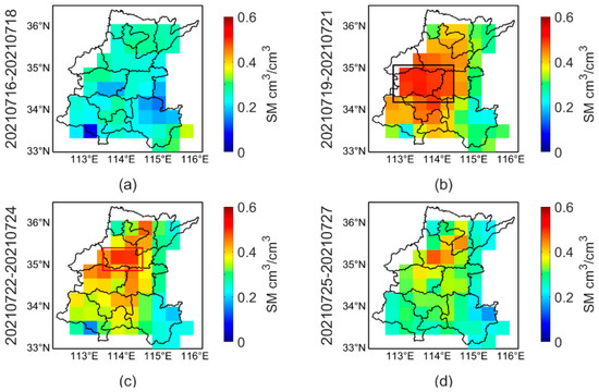
Figure 10. (a–d) are the changes in soil moisture obtained from SMAP before and after the flood (from 16 July to 27 July 2021).

Compared to Figure 9a, from19 July to 24 July 2021, the brightness temperature changes of the black box in Figure 9b and the red box in Figure 9c were more obvious. Compared to Figure 10a, from 19 July to 24 July 2021, the soil moisture of the black box in Figure 10b and the red box in Figure 10c also changed. It shows that the duration of the flood is from 19 July to 24 July 2021, and the area corresponding to the black box (Zhengzhou) and the area corresponding to the red box (Xinxiang) are also severely affected areas. Therefore, based on the changes of SMAP brightness temperature and soil moisture, the occurrence of floods and the affected areas can be monitored.

In addition, SMAP time-series data on brightness temperature and soil moisture from 1 July to 15 August 2021, were collected for the study area to see the changes in both types of data before, during and after the flood. Surface brightness temperature and soil moisture values from the sampled pixel of the affected areas were plotted to see the response of the brightness temperature and soil moisture to the flood. Similar to [37], the median of all grids was selected as the threshold between the water and the land during the flood period (from 19 July to 24 July 2021). As shown in Figure 11, the threshold is 248 K for using brightness temperature data for time-series analysis. For using soil moisture data for the time-series analysis, the threshold is 0.38 cm³/cm³ which is similar to that used in [37].

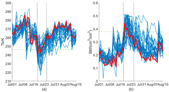
Figure 11. (a) Surface brightness temperature of the grid from the 11 cities. (b) Surface soil moisture of the grid from the 11 cities.The red line indicates the median of the grid. The green dashed line represents the threshold (248 K and 0.38 cm³/cm³). The blue line represents the time series change of bright temperature (a) and soil moisture (b) of the grid. The black dashed line is from 19 July to 24 July 2021.

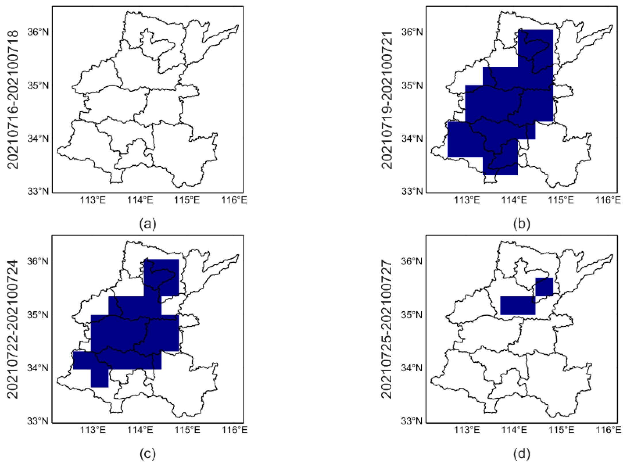
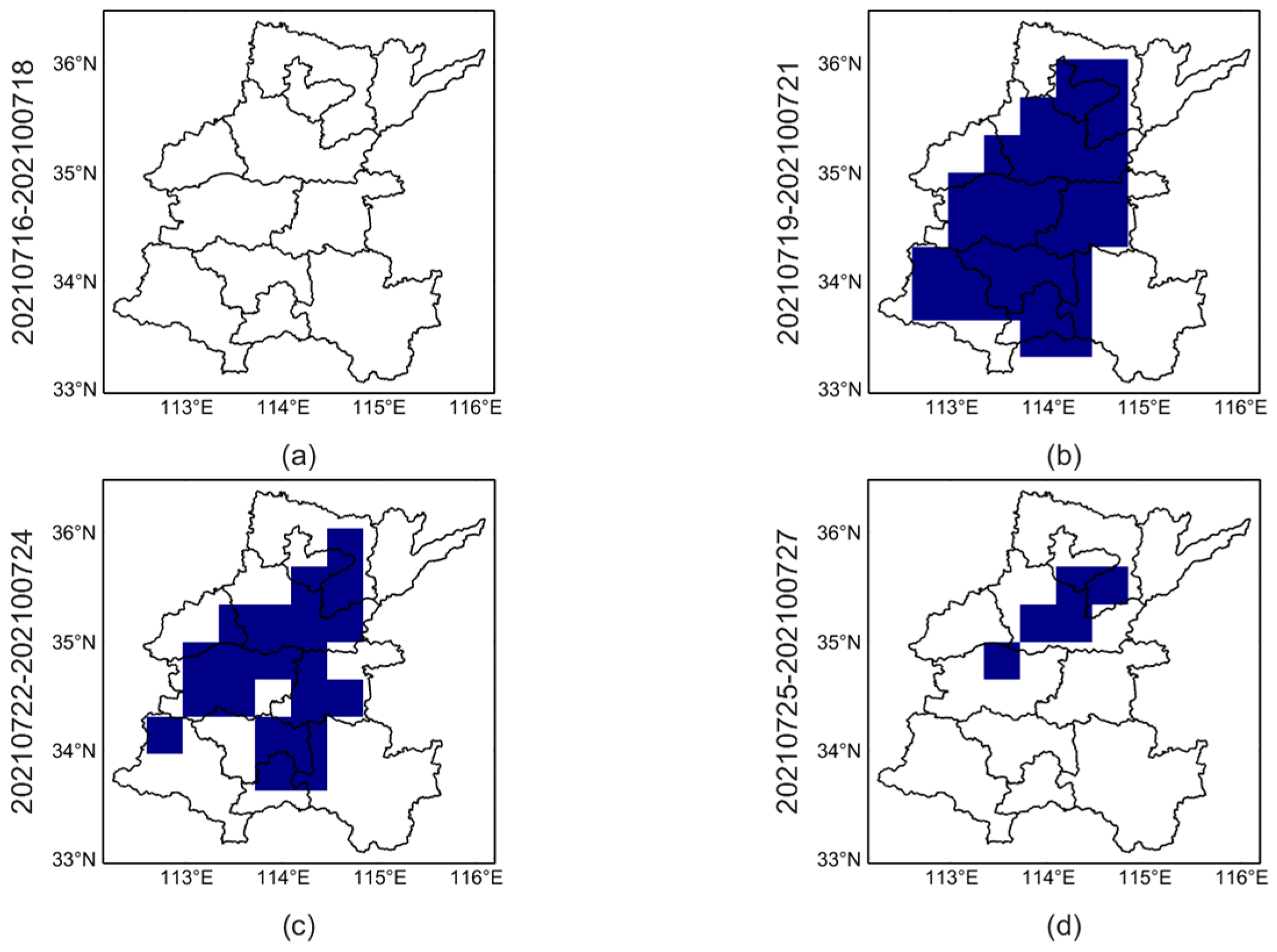
Figure 12 and Figure 13 are the inundated area maps drawn by SMAP brightness temperature and soil moisture, respectively (from 16 July to 27 July 2021). Based on the estimates from the SMAP observations, the approximate change in the flood and the inundated areas can be detected. Like [25], it also proved that SMAP can also monitor floods.

Figure 12. (a–d) are using the threshold (248 K) of the brightness temperature to monitor changes in the inundated area.

Figure 13. (a–d) are using the threshold (0.38 cm³/cm³) of soil moisture to monitor changes in the inundated area.

3.5. Comparison with SMAP

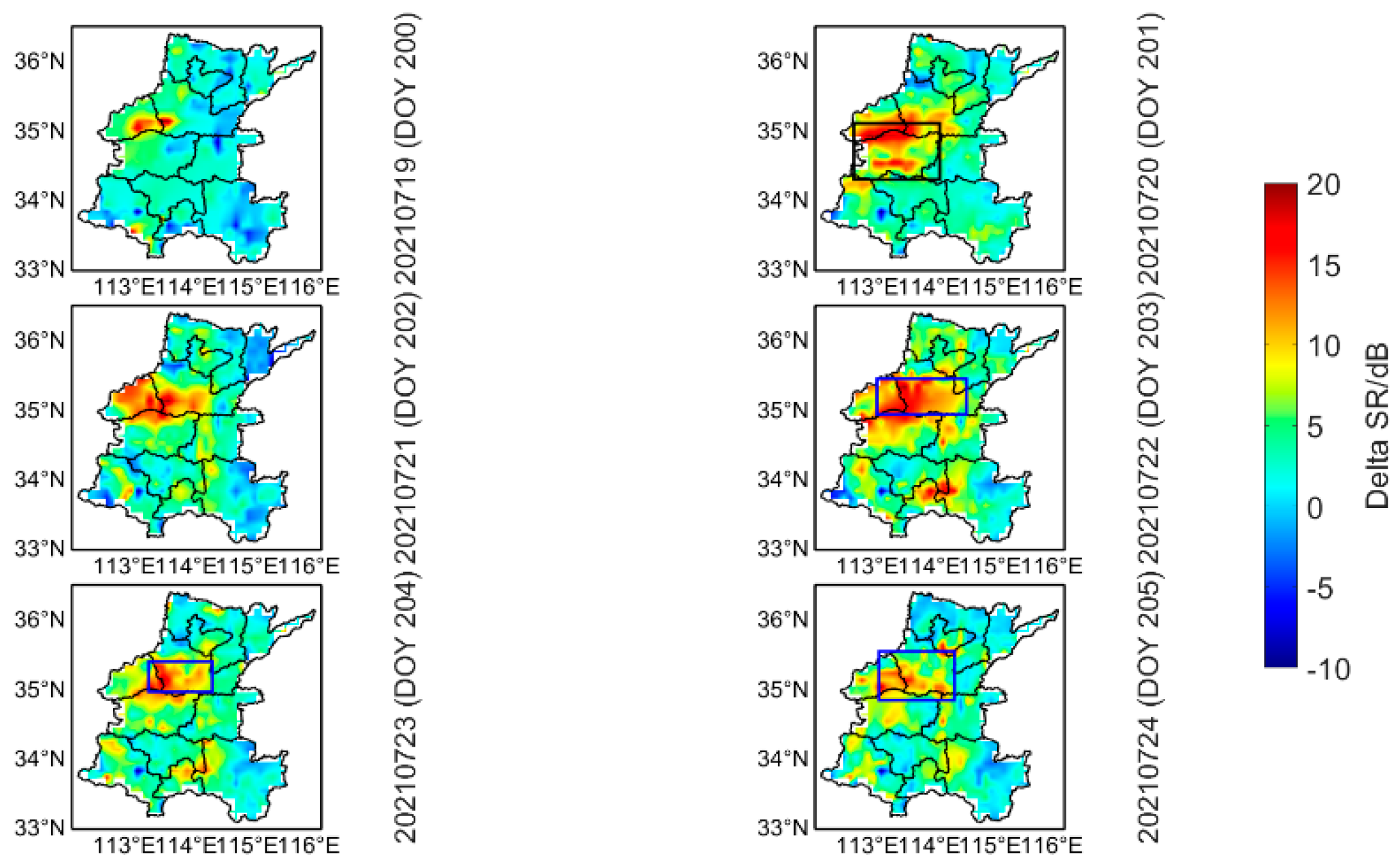
In order to compare CYGNSS and SMAP, as shown in Figure 14, Figure 15 and Figure 16, we respectively made temporal changes of CYGNSS reflectivity and brightness temperature and soil moisture from SMAP during and before the flood (on 18 July 2021).

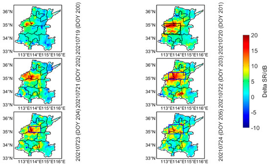
Figure 14. The amount of change in CYGNSS reflectivity from 19 July to 24 July 2021 and before (on 18 July 2021) the flood.

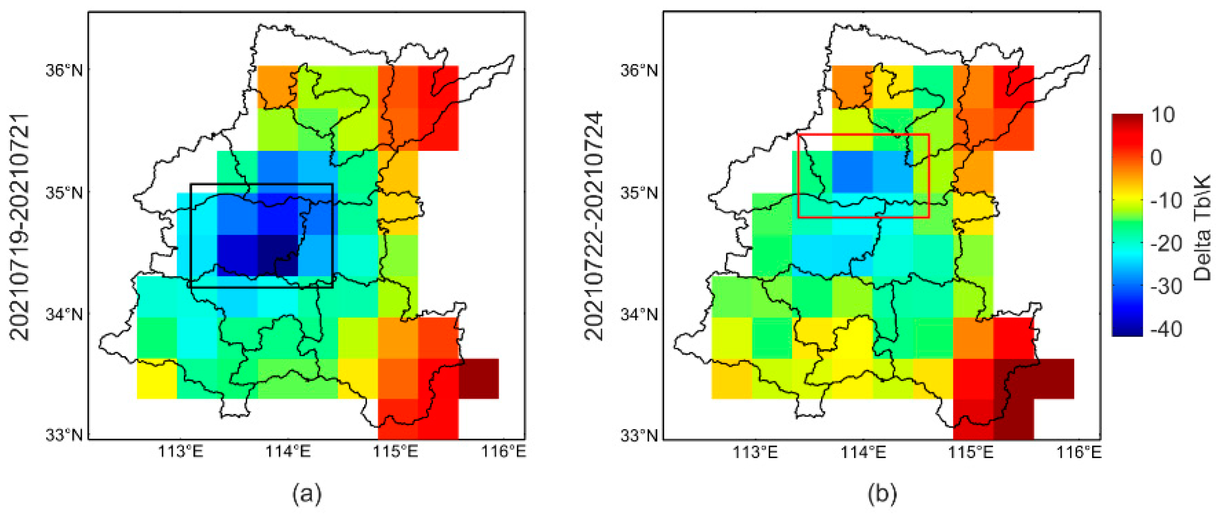
Figure 15. (a,b) are the amount of change in the brightness temperature from 19 July to 24 July 2021 and before the flood (from 16 July to 18 July 2021).

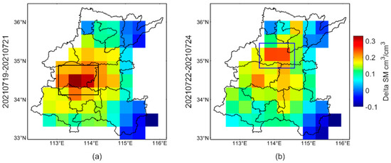
Figure 16. (a,b) are the amount of change in the soil moisture from 19 July to 24 July 2021 and before the flood (from 16 July to 18 July 2021).

It can be seen from Figure 14 that the changes of CYGNSS reflectivity in the black box and the blue box are obvious, and the maximum change is 15.7 dB. Correspondingly, in Figure 15 and Figure 16, the maximum change in the brightness temperature is 40.2 K, and the maximum change in the soil moisture is 0.33 cm³/cm³. As shown in Figure 14, the area of the black box (on 20 July 2021) represents Zhengzhou, which is consistent with the area represented by the black boxes in Figure 15 and Figure 16. From 22 July to 24 July 2021, the area represented by the blue box is Xinxiang, which is consistent with the area represented by the red box in Figure 15 and the blue box in Figure 16. This shows that the monitoring results of CYGNSS are in good agreement with SMAP.

3.6. Comparison with Remote Sensing Images

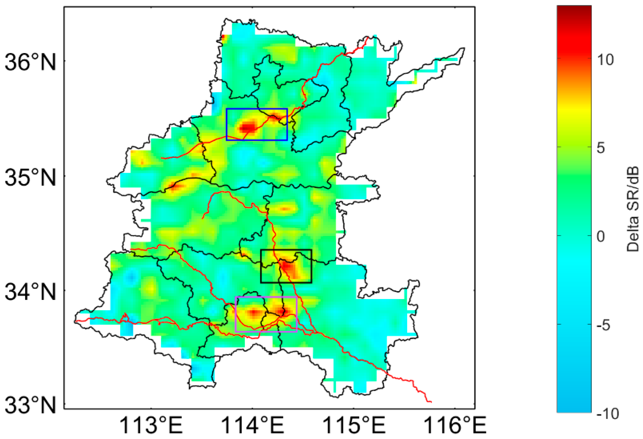
It can be seen from Figure 2 that the flood was mainly concentrated in Xinxiang. By observing the amount of change in CYGNSS reflectivity before and after the flood (see Figure 17), it is possible to estimate the area that was most severely affected by the flood.

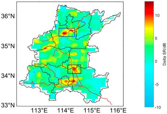
Figure 17. The amount of change in CYGNSS reflectivity before (on 18 July 2021) and after (on 26 July 2021) the flood.

In Figure 17, from top to bottom, the red jagged lines represent the Wei River, Jialu River, Ying River, and Sha River. It can be seen from Figure 17 that the reflectivity of the flood discharge area (black box) affected by flood discharge of the Jialu River and the flood discharge area (purple box) affected by flood discharge of the Sha River and Ying River are more obvious, indicating that the disaster situation is serious. In Xinxiang (blue Box), the changes are more apparent. This is due to extreme weather moving northwards from Zhengzhou and dropping 26 cm (10 inches) of rain in Xinxiang within two hours. In addition, there are many rivers and reservoir networks in the area, so it is greatly affected by the flood.

Thus, based on the estimates from the CYGNSS observations, the data on the areas severely affected by the flood are also consistent with the optical image in Figure 2.

4. Discussion

We applied quality control on the CYGNSS data to remove outliers. Then the CY- GNSS measurements with a period of one day were gridded. Afterwards, we obtained the occurrence and the duration of the flood based on the CYGNSS observations. In the next step, a simple threshold method was used to monitor the inundated areas as well as the shift and distribution of the areas severely affected by the flood. For inundated areas, using different thresholds will lead to different results. In general, the threshold is related to the terrain and vegetation coverage of the study area. More studies are needed to test the influence of vegetation and roughness on the threshold.

Similarly, based on the brightness temperature and soil moisture changes from SMAP, we generated a temporal map to show the evolution of the flood. However, the monitoring results are limited by the temporal resolution of SMAP. There may also be differences with CYGNSS in terms of the occurrence and duration of floods.

When the flood occurred, the brightness temperature, soil moisture from SMAP and CYGNSS reflectivity changed obviously in Zhengzhou and Xinxiang. This shows that their monitoring results are in good agreement. The daily changes are not captured by SMAP; in contrast, CYGNSS can provide daily monitoring results, and the spatial resolution is also better than SMAP. It is, therefore, obvious that CYGNSS high temporal and spatial resolution data can monitor floods in more detail and faster. Comparing the change of CYGNSS reflectivity with the optical image, it is also found that they are in good agreement. It further proves that the CYGNSS results are relatively accurate and can be applied to flood monitoring.

5. Conclusions

We used spaceborne GNSS-R data (CYGNSS Level 1 Science Data products) as observations to detect and map the Henan flood. We obtained the reflectivity by calculating the bistatic radar equation. Afterwards, taking into account that reflectivity was sensitive to inland surface water, the CYGNSS reflectivity was corrected and used to monitor the flood. By calculating the amount of change in the CYGNSS reflectivity before and after the flood, and verifying it with the MODIS optical image and SMAP, we monitored the main affected areas. The results show that the monitoring of flood changes based on CYGNSS observations is consistent with the SMAP results. Notably, spaceborne GNSS-R data with high temporal and spatial resolution can achieve rapid flood monitoring and inundated area mapping, which can help relevant departments in emergency management (determine risk areas, exercise safe evacuation options, and update response plans). Although CYGNSS is designed to observe ocean surface wind speed during hurricanes, this study further confirms that CYGNSS data can also be applied to land surface remote sensing and has high application value in hydrology and agriculture. Future GNSS-R missions will be capable of collecting reflected signals from GNSS constellations and will provide more detailed information to help flood studies.

References

- Messner, F.; Meyer, V. Flood damage, vulnerability and risk perception–challenges for flood damage research. In Flood Risk Management: Hazards, Vulnerability and Mitigation Measures; Springer: Berlin/Heidelberg, Germany, 2006; pp. 149–167. [Google Scholar]
- Diakakis, M.; Boufidis, N.; Grau, J.M.; Andreadakis, E.; Stamos, I. A systematic assessment of the effects of extreme flash floods on transportation infrastructure and circulation: The example of the 2017 Mandra flood. Int. J. Disaster Risk Reduct. 2020, 47, 101542. [Google Scholar] [CrossRef]
- Sharafi, S.; Kamangir, H.; King, S.A.; Safaierad, R. Effects of extreme floods on fluvial changes: The Khorramabad River as case study (western Iran). Arab. J. Geosci. 2021, 14, 1–11. [Google Scholar] [CrossRef]
- Davenport, F.V.; Burke, M.; Diffenbaugh, N.S. Contribution of historical precipitation change to US flood damages. Proc. Natl. Acad. Sci. USA 2021, 118, e2017524118. [Google Scholar] [CrossRef]
- Nofal, O.M.; van de Lindt, J.W. High-resolution flood risk approach to quantify the impact of policy change on flood losses at community-level. Int. J. Disaster Risk Reduct. 2021, 62, 102429. [Google Scholar] [CrossRef]
- Shahabi, H.; Shirzadi, A.; Ghaderi, K.; Omidvar, E.; Al-Ansari, N.; Clague, J.J.; Geertsema, M.; Khosravi, K.; Amini, A.; Bahrami, S.; et al. Flood Detection and Susceptibility Mapping Using Sentinel-1 Remote Sensing Data and a Machine Learning Approach: Hybrid Intelligence of Bagging Ensemble Based on K-Nearest Neighbor Classifier. Remote. Sens. 2020, 12, 266. [Google Scholar] [CrossRef] [Green Version]
- Costache, R.; Arabameri, A.; Blaschke, T.; Pham, Q.B.; Pham, B.T.; Pandey, M.; Arora, A.; Linh, N.T.T.; Costache, I. Flash-Flood Potential Mapping Using Deep Learning, Alternating Decision Trees and Data Provided by Remote Sensing Sensors. Sensors 2021, 21, 280. [Google Scholar] [CrossRef] [PubMed]
- Platnick, S.; King, M.D.; Ackerman, S.A.; Menzel, W.P.; Baum, B.A.; Riedi, J.C.; Frey, R.A. The MODIS cloud products: Algorithms and examples from terra. IEEE Trans. Geosci. Remote. Sens. 2003, 41, 459–473. [Google Scholar] [CrossRef] [Green Version]
- Drusch, M.; Del Bello, U.; Carlier, S.; Colin, O.; Fernandez, V.; Gascon, F.; Hoersch, B.; Isola, C.; Laberinti, P.; Martimort, P.; et al. Sentinel-2: ESA’s Optical High-Resolution Mission for GMES Operational Services. Remote. Sens. Environ. 2012, 120, 25–36. [Google Scholar] [CrossRef]
- Kuenzer, C.; Guo, H.; Huth, J.; Leinenkugel, P.; Li, X.; Dech, S. Flood Mapping and Flood Dynamics of the Mekong Delta: ENVISAT-ASAR-WSM Based Time Series Analyses. Remote. Sens. 2013, 5, 687–715. [Google Scholar] [CrossRef] [Green Version]
- Rodriguez-Alvarez, N.; Camps, A.; Vall-llossera, M.; Bosch-Lluis, X.; Monerris, A.; Ramos-Perez, I.; Valencia, E.; Marchan-Hernandez, J.F.; Martinez-Fernandez, J.; Baroncini-Turricchia, G.; et al. Land Geophysical Parameters Retrieval Using the Interference Pattern GNSS-R Technique. IEEE Trans. Geosci. Remote. Sens. 2011, 49, 71–84. [Google Scholar] [CrossRef]
- Hein, G.W. Status, perspectives and trends of satellite navigation. Satell. Navig. 2020, 1, 1–12. [Google Scholar] [CrossRef]
- Ruf, C.; Chang, P.; Clarizia, M.P.; Gleason, S.; Jelenak, Z.; Murray, J.; Morris, M.; Musko, S.; Posselt, D.; Provost, D.; et al. CYGNSS Handbook; Michigan Pub.: Ann Arbor, MI, USA, 2016; Volume 154, p. 1. [Google Scholar]
- Chew, C.; Small, E. Soil moisture sensing using spaceborne GNSS reflections: Comparison of CYGNSS reflectivity to SMAP soil moisture. Geophys. Res. Lett. 2018, 45, 4049–4057. [Google Scholar] [CrossRef] [Green Version]
- Chew, C.C.; Small, E.E.; Larson, K.M.; Zavorotny, V.U. Effects of Near-Surface Soil Moisture on GPS SNR Data: Development of a Retrieval Algorithm for Soil Moisture. IEEE Trans. Geosci. Remote. Sens. 2014, 52, 537–543. [Google Scholar] [CrossRef]
- Cartwright, J.; Banks, C.J.; Srokosz, M. Sea Ice Detection Using GNSS-R Data from TechDemoSat-1. J. Geophys. Res. Ocean. 2019, 124, 5801–5810. [Google Scholar] [CrossRef]
- Gao, F.; Xu, T.; Meng, X.; Wang, N.; He, Y.; Ning, B. A Coastal Experiment for GNSS-R Code-Level Altimetry Using BDS-3 New Civil Signals. Remote. Sens. 2021, 13, 1378. [Google Scholar] [CrossRef]
- Liu, W.; Beckheinrich, J.; Semmling, M.; Ramatschi, M.; Vey, S.; Wickert, J.; Hobiger, T.; Haas, R. Coastal Sea-Level Measurements Based on GNSS-R Phase Altimetry: A Case Study at the Onsala Space Observatory, Sweden. IEEE Trans. Geosci. Remote. Sens. 2017, 55, 5625–5636. [Google Scholar] [CrossRef]
- Al-Khaldi, M.M.; Johnson, J.T.; O’Brien, A.J.; Balenzano, A.; Mattia, F. Time-Series Retrieval of Soil Moisture Using CYGNSS. IEEE Trans. Geosci. Remote. Sens. 2019, 57, 4322–4331. [Google Scholar] [CrossRef]
- Camps, A.; Park, H.; Castellví, J.; Corbera, J.; Ascaso, E. Single-Pass Soil Moisture Retrievals Using GNSS-R: Lessons Learned. Remote. Sens. 2020, 12, 64. [Google Scholar] [CrossRef]
- Chew, C.; Small, E. Description of the UCAR/CU Soil Moisture Product. Remote. Sens. 2020, 12, 1558. [Google Scholar] [CrossRef]
- Asharaf, S.; Waliser, D.E.; Posselt, D.J.; Ruf, C.S.; Zhang, C.; Putra, A.W. CYGNSS Ocean Surface Wind Validation in the Tropics. J. Atmos. Ocean. Technol. 2021, 38, 711–724. [Google Scholar] [CrossRef]
- Li, X.; Yang, D.; Yang, J.; Zheng, G.; Han, G.; Nan, Y.; Li, W. Analysis of coastal wind speed retrieval from CYGNSS mission using artificial neural network. Remote. Sens. Environ. 2021, 260, 112454. [Google Scholar] [CrossRef]
- Chew, C.; Reager, J.T.; Small, E. CYGNSS data map flood inundation during the 2017 Atlantic hurricane season. Sci. Rep. 2018, 8, 9336. [Google Scholar] [CrossRef] [PubMed]
- Wan, W.; Liu, B.; Zeng, Z.; Chen, X.; Wu, G.; Xu, L.; Chen, X.; Hong, Y. Using CYGNSS Data to Monitor China’s Flood Inundation during Typhoon and Extreme Precipitation Events in 2017. Remote. Sens. 2019, 11, 854. [Google Scholar] [CrossRef] [Green Version]
- Pan, Y.; Ren, C.; Liang, Y.; Zhang, Z.; Shi, Y. Inversion of surface vegetation water content based on GNSS-IR and MODIS data fusion. Satell. Navig. 2020, 1, 1–15. [Google Scholar] [CrossRef]
- Ruf, C.S.; Atlas, R.; Chang, P.S.; Clarizia, M.P.; Garrison, J.L.; Gleason, S.; Katzberg, S.J.; Jelenak, Z.; Johnson, J.T.; Majumdar, S.J. New ocean winds satellite mission to probe hurricanes and tropical convection. Bull. Am. Meteorol. Soc. 2016, 97, 385–395. [Google Scholar] [CrossRef]
- Ruf, C.; Asharaf, S.; Balasubramaniam, R.; Gleason, S.; Lang, T.; McKague, D.; Twigg, D.; Waliser, D. In-orbit performance of the constellation of CYGNSS hurricane satellites. Bull. Am. Meteorol. Soc. 2019, 100, 2009–2023. [Google Scholar] [CrossRef]
- Yan, Q.; Huang, W.; Jin, S.; Jia, Y. Pan-tropical soil moisture mapping based on a three-layer model from CYGNSS GNSS-R data. Remote. Sens. Environ. 2020, 247, 111944. [Google Scholar] [CrossRef]
- Zavorotny, V.U.; Voronovich, A.G. Scattering of GPS signals from the ocean with wind remote sensing application. IEEE Trans. Geosci. Remote. Sens. 2000, 38, 951–964. [Google Scholar] [CrossRef] [Green Version]
- Kim, H.; Lakshmi, V. Use of Cyclone Global Navigation Satellite System (CyGNSS) Observations for Estimation of Soil Moisture. Geophys. Res. Lett. 2018, 45, 8272–8282. [Google Scholar] [CrossRef] [Green Version]
- Richards, J. Microwave Radar and Radiometric Remote Sensing. IEEE Geosci. Remote. Sens. Mag. 2015, 3, 51–52. [Google Scholar] [CrossRef]
- Voronovich, A.G.; Zavorotny, V.U. Bistatic radar equation for signals of opportunity revisited. IEEE Trans. Geosci. Remote. Sens. 2017, 56, 1959–1968. [Google Scholar] [CrossRef]
- Van Dijk, A.I.; Brakenridge, G.R.; Kettner, A.J.; Beck, H.E.; De Groeve, T.; Schellekens, J. River gauging at global scale using optical and passive microwave remote sensing. Water Resour. Res. 2016, 52, 6404–6418. [Google Scholar] [CrossRef]
- Entekhabi, D.; Das, N.; Njoku, E.; Johnson, J.; Shi, J. Soil Moisture Active Passive (SMAP) Algorithm Theoretical Basis Document L2 & L3 radar/radiometer soil moisture (active/passive) data products. Initial Release 2012, 1, 71. [Google Scholar]
- Carreno-Luengo, H.; Luzi, G.; Crosetto, M. Sensitivity of CyGNSS Bistatic Reflectivity and SMAP Microwave Radiometry Brightness Temperature to Geophysical Parameters Over Land Surfaces. IEEE J. Sel. Top. Appl. Earth Obs. Remote. Sens. 2019, 12, 107–122. [Google Scholar] [CrossRef]
- Rahman, M.S.; Di, L.; Shrestha, R.; Eugene, G.Y.; Lin, L.; Zhang, C.; Hu, L.; Tang, J.; Yang, Z. Agriculture flood mapping with Soil Moisture Active Passive (SMAP) data: A case of 2016 Louisiana flood. In Proceedings of the 2017 6th International Conference on Agro-Geoinformatics, Fairfax, VA, USA, 7–10 August 2017; pp. 1–6. [Google Scholar]
Publisher’s Note: MDPI stays neutral with regard to jurisdictional claims in published maps and institutional affiliations. |
© 2021 by the authors. Licensee MDPI, Basel, Switzerland. This article is an open access article distributed under the terms and conditions of the Creative Commons Attribution (CC BY) license (https://creativecommons.org/licenses/by/4.0/).