Abstract
The Yangtze River Delta (YRD) is one of the regions with the most intensive human activities. The eutrophication of lakes in this area is becoming increasingly serious with consequent negative impacts on the water supply of the surrounding cities. But the spatial-temporal characteristics and driving factors of the trophic state of the lake in this region are still not clearly addressed. In this study, a semi-analytical algorithm for estimating the trophic index (TSI) using particle absorption at 645 nm based on MODIS images is proposed to monitor and evaluate the trophic state of 41 large lakes (larger than 10 km2) in the YRD from 2002 to 2020. The performance of the proposed algorithm is evaluated using an independent dataset. Results showed that the root-mean-square error (RMSE) of the algorithm is less than 6 and the mean absolute percentage error (MAPE) does not exceed 8%, indicating that it can be applied for remotely deriving the TSI in the YRD. The spatial-temporal patterns revealed that there were significantly more lakes with moderate eutrophication in the Lower Yangtze River (LYR) than in the Lower Huaihe River (LHR). The overall average value of the TSI reaches a maximum in summer and a minimum in winter. The TSI value in the YRD over the period 2002–2020 showed a downward trend, especially after 2013. Individually, 33 lakes showed a downward trend and 8 lakes showed an upward trend. Furthermore, marked seasonal and interannual temporal variations can be clearly observed in the LYR and LHR and the sum of the variance contributions of seasonal and interannual components is more than 50%. Multiple linear regression analysis showed that human activities can explain 65% of the variation in the lake TSI in the YRD.
1. Introduction
The Yangtze River Delta (YRD) is located in the eastern coastal area of rapid economic development in China. Four of the ten largest freshwater lakes in China are in this region. With the acceleration of economic development and industrialization in the YRD, the degree of lake eutrophication is gradually increasing [1]; for example, the chlorophyll-a (Chla) concentration in Lake Taihu increased sharply from 2003 to 2007 (its peak value), decreased from 2007 to 2009, then increased slightly from 2009 to 2013 [2]. Meanwhile, the severe algal blooms (coverage area > 80 km2) in Lake Chaohu in 2007 were significantly more severe than in other years [3]. In summary, lake eutrophication is becoming a critical issue for the water environment [4,5,6] and it is urgent to understand the spatial-temporal variation pattern of lake trophic state in the YRD. Research on the temporal and spatial characteristics of lake trophic state in the YRD is helpful to reveal the changes in lake water quality in this region and plays a vital role in the supervision and management of lake ecosystems.
To assess the trophic state of lakes, the trophic state index (TSI) based on multiple water quality parameters is widely adopted [4,7]. Measurement of TSI parameters requires on-site water sample collection, transportation, sample filtration, and chemical analysis [8]. This direct, labor intensive approach greatly limits the rapid assessment and characterization of the trophic state in inland waters on a large scale. With the development of remote sensing technology, an increasing number of satellite sensors have been applied to observe the trophic state of lakes [5,6,9]. Remote sensing technology provides an effective way to monitor trophic state in whole lake, regional, or even global lakes.
Since Wezernak [10] proposed the concept of a TSI based on remote sensing in 1976, various scholars have performed much research on remote sensing assessments of the TSI [4,11,12]. Olmanson [11] built a 20-year water clarity database for Minnesota lakes and derived lake eutrophication through the Secchi disk depth (SDD) indicator. Song [12] established algorithms for remote estimation of total phosphorus (TP), Chla, and SDD then evaluated the trophic state using these three trophic indicators. Guan [4] proposed a machine learning-based piecewise algorithm for Chla then used remotely sensed Chla and algal bloom areas to classify the eutrophication state of 50 large lakes in the Yangtze Plain. In summary, this kind of method usually retrieves one or more trophic indicators by remote sensing then calculates the TSI based on their values. However, it is still a great challenge to accurately estimate the needed parameters for calculating the TSI in inland waters [13]. This uncertainty will bring a certain degree of deviation from the real result. At the same time, the algorithms for estimating trophic indicators, such as SDD, Chla, TP, and TN, often have a certain regionality and poor transferability. Therefore, it is urgent to develop a novel remote sensing method for retrieving the TSI using satellite images that is more accurate and consistent. Numerous studies have shown that there is a strong correlation between the TSI and the absorption of optically active substances [6,14,15]. Shi [6] used nonwater absorption at 440 nm (at-w(440)) to retrieve the TSI from Landsat images in inland waters. This new attempt to derive the TSI from the total absorption coefficient of optically active components is only applied to Lake Qiandao. It is well known that Lake Qiandao is very clear, and its optical features are obviously different from those of other eutrophic lakes [16]. According to our in-situ data, the performance of this algorithm applied in other lakes with different bio-optical properties still needs to be improved. Therefore, it is very important to propose a suitable method to retrieve the trophic state of lakes in the YRD.
In addition, many studies have been conducted on long-term spatial-temporal TSI variation features [4,9]. Chen [9] applied the proposed model to Landsat 8 OLI images to obtain the temporal and spatial distributions of the TSI in three typical lakes from 2013 to 2018. Guan [4] studied the eutrophication state of lakes in the Yangtze River Plain from 2003 to 2011 and 2017 to 2018. However, these studies are either short in duration or the study years are not continuous, limiting the phenomena that may be revealed and the conclusions that may be drawn.
To better understand the spatial-temporal variation in lake trophic state in the YRD, the objectives of this study are to (1) develop a remote sensing method for monitoring the TSI of lakes on a large scale, (2) reveal the spatial-temporal trophic state variation of the lakes in the YRD from 2002 to 2020 using MODIS images, and (3) analyze the contribution of human activities to the variation in lake trophic state in the YRD.
2. Materials and Methods
2.1. Study Area and Datasets
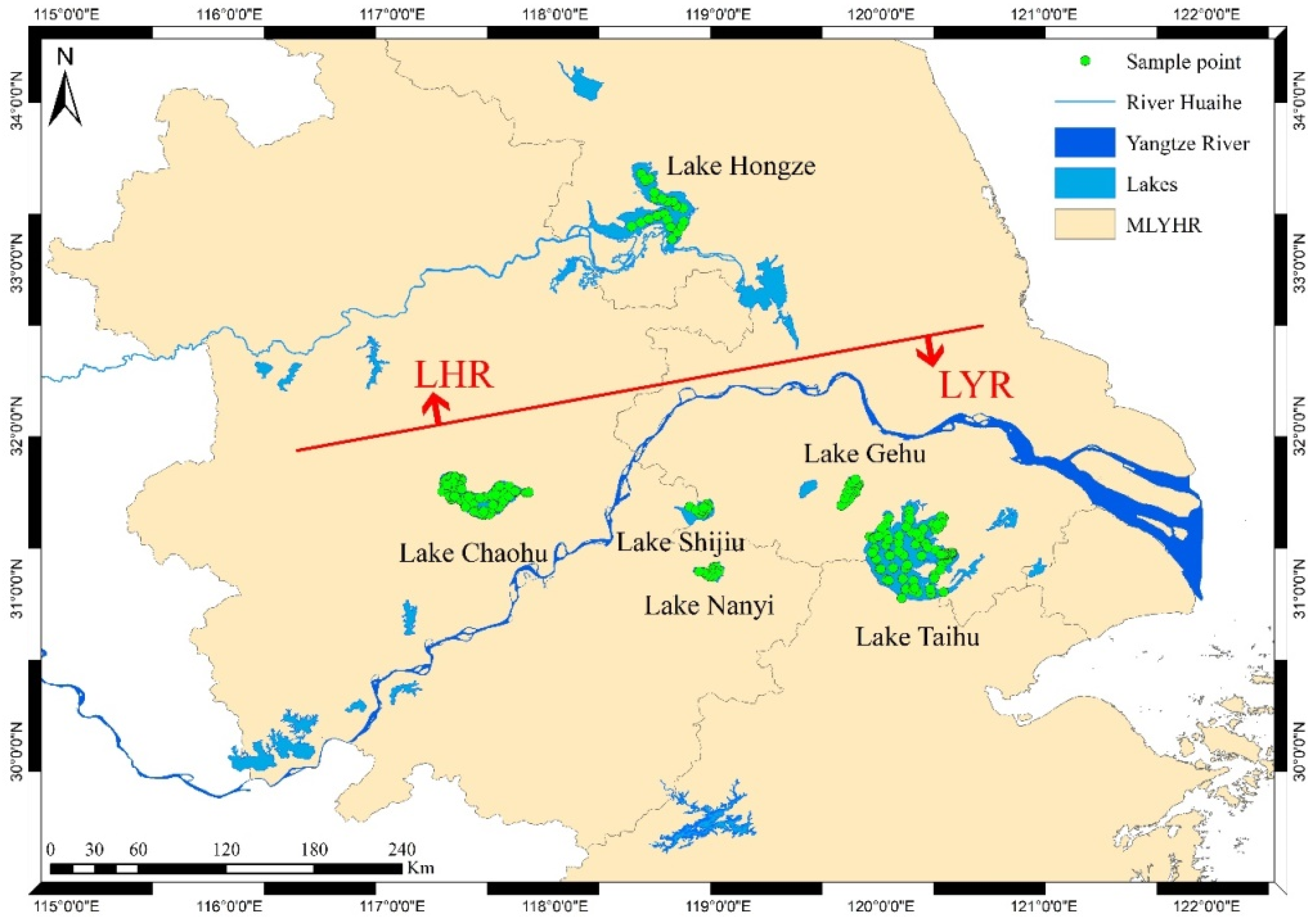
The YRD (Figure 1) is located in the lower reaches of the Yangtze River in China, bordering the Yellow Sea and the East China Sea. It is China’s largest area of urban agglomeration and the most economically active region, contributing 23.5% of the gross domestic product [17]. Taking the Jianghuai Watershed and Tongyang Canal as the boundary (simply indicated by a red line in Figure 1), the YRD can be divided into the lower Huai River (LHR) part and the lower Yangtze River (LYR) part. The YRD region has many river networks and a large number of lakes, with a total number of more than 200 lakes with an area ranging from 0.01 km2 to more than 2000 km2. These provide important water resources for the YRD region [18,19]. Most of these lakes are shallowly turbid lakes with algal blooms and man-made sand mining activities, resulting in large spatiotemporal variability in suspended particulates and phytoplankton [20]. In this study, due to the satellite image spatial resolution, 41 lakes with an area larger than 10 km2 in the YRD were selected to study trophic state variation characteristics.

Figure 1.
Study area and sampling point distribution.
From 2016 to 2019, a total of 286 water samples were collected from three lakes (Lake Taihu, Lake Chaohu, and Lake Hongze) during 9 cruises in different seasonal conditions. An independent dataset (N = 35) collected from Lake Shijiu, Lake Nanyi, and Lake Gehu in October 2020 is applied to validate the applicability of the algorithm in other lakes in the YRD.
At each sampling point, a 2 L surface water sample was collected and remote sensing reflectance (Rrs) and SDD were measured. Rrs was acquired from above-surface measurements using an Analytical Spectral Devices (ASD) field spectrometer [21]. SDD was obtained in the field using a Secchi disk.
The water samples collected in the field were preserved at a low temperature and immediately transported to the laboratory for analysis on the same day. Chla, TP, and total suspended matter concentration (TSM) were examined in the laboratory. The concentration of Chla was measured by using a hot ethanol spectrophotometer method. The concentration of TSM was determined by drying, baking, and weighing according to the GB11901-89 standard [20]. TP was examined by spectrophotometry (Shimadzu, UV-3600) after digestion with alkaline potassium persulfate [22]. In addition, the absorption coefficients of total particulate matter (ap), phytoplankton (aph), and nonalgal particles (anap) were measured by using the quantitative filter technique (QFT) [23].
2.2. MODIS Image Preprocessing
MODIS Aqua Daily Reflectance Product data (MYD09) provide land surface spectral reflectance with a 500 m spatial resolution at seven bands (central wavelengths are 645 nm, 859 nm, 469 nm, 555 nm, 1240 nm, 1640 nm, and 2130 nm). This product is a rasterized secondary data product (L2G) in which atmospheric and aerosol correction has been performed based on low-level data products [24]. Some studies have demonstrated that this product can sometimes be directly used for remote sensing retrieval of water quality parameters [6,25]. However, due to the optical complexity of inland waters and aerosols over inland waters, this MODIS product often fails [26].
Therefore, a simple and operational correction method based on the near-infrared (NIR) and short-wave infrared (SWIR) bands for MODIS products proposed by Wang [27] was used to perform remote sensing reflectivity correction for this study. To validate the atmospheric correction accuracy in the YRD, the in-situ measured Rrs of 134 synchronized sampling points with satellite overpass date were compared with the Rrs derived from the atmospheric corrected image. Moreover, two often used methods for atmospheric correction in inland turbid waters, shortwave infrared (SWIR) [28] and the management unit of the North Seas Mathematical Models (MUMM) [29], were also selected for comparison with this method. The simple and operational correction method is shown in Equation (1):
where R(λ) is the reflectivity of MYD09 at λ wavelength, min (RNIR:RSWIR) is the minimum band value at NIR and SWIR, and π is set as the denominator. Equation (1) converts surface reflectivity into out-of-water reflectivity.
The floating algae index (FAI) [30] was applied to mask the algal bloom area by using the criteria of FAI > −0.004.
2.3. Trophic State Index
Carlson [31] developed the TSI based on SDD, Chla, and TP to evaluate lake trophic state. The specific calculation formula is shown in Equations (2)–(4). The traditional TSI evaluation is expressed by a numerical value between 0–100. When the TSI was less than 30, it was considered an oligotrophic state; when 30 < TSI < 50, the water was considered a mesotrophic state; and when the TSI > 50, the water was considered a eutrophic state. Eutrophic level can be subdivided into mild eutrophic state (50 < TSI < 60), moderate eutrophic state (60 < TSI < 70) and hypereutrophic state (TSI > 70). The TSI for this paper was calculated using three water quality indices: Chla, SD, and TP. In Equation (5), we recalibrated the coefficients of each water quality index.
2.4. The Analysis Method and Data for Long-Term Changes of TSI
The ensemble empirical mode decomposition method (EEMD) was used to analyze the time-series variation in the TSI in the YRD. EEMD is an auxiliary noise data analysis method that is widely used to study the long-term changes of research objects [32]. The result of the integrated mean can be used as the final result (see Equations (6) and (7)).
where Xj(t) is the new time signal, Pj(t) is Gaussian white noise, and X(t) is the original signal sequence.
To analyze the driving force of TSI long-term varying trends in the YRD, two categories of data were selected for analysis. The climatic data, including temperature, rainfall, and wind speed, were downloaded from the nearest meteorological station to each lake at the China Meteorological Data Service Centre (https://data.cma.cn/en, accessed on 14 July 2021), and annual meteorological data were obtained from average monthly data. The other kind of data used, on human activity, including fertilizer consumption and industrial wastewater, come from the statistical yearbook of each province. At the same time, a multiple linear regression model was employed to determine the main driving forces and quantify the relative contribution of explanatory variables to the long-term trend of TSI [33,34,35].
2.5. The Derivation of the Particle Absorption Coefficient
In this study, the absorption of phytoplankton was used to develop the TSI estimation algorithm; therefore, the semi-analytical algorithm (denoted as QAA645-ap) was modified from QAA [36] to derive the particle absorption coefficients. QAA645-ap can derive the absorption and backscattering coefficients by analytically inverting the spectral remote-sensing reflectance (Rrs(λ)). As shown in Figure 2, first, the two intermediate variables rrs(λ) and u(λ) were derived based on the method proposed by Lee [36]. Second, the total absorption coefficient (a) at a reference wavelength (λ0) was calculated followed by the value of the total backscattering coefficient (bb) at a reference wavelength (λ0). Third, solving the formula for bb at the reference wavelength can obtain bb at the specified wavelength. Finally, based on the total absorption of water components at the given wavelength, the component absorption coefficients (phytoplankton pigments, nonpigmented particles, and yellow substance) can be further algebraically decomposed from the total absorption coefficient. Furthermore, according to the relationship between the TSI and the absorption coefficient, the TSI of the YRD can be estimated.
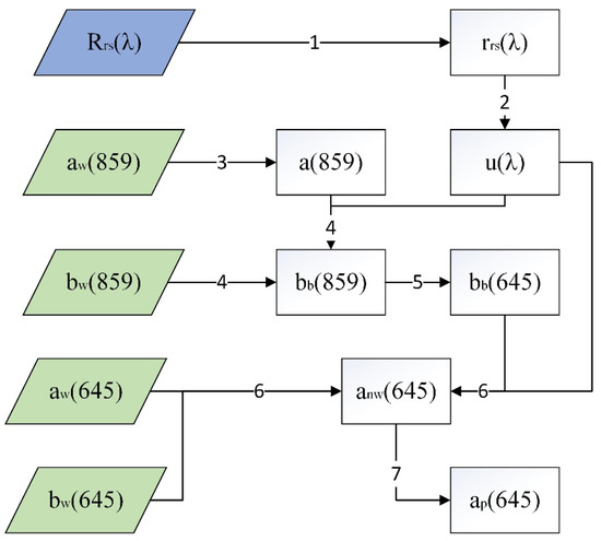
Figure 2.
Flow chart of the estimation method of particle absorption at 645 nm.
The detailed procedure for deriving ap(645) from the nadir-viewing spectral remote-sensing reflectance just below the surface (rrs) is shown in Table 1.

Table 1.
Steps of QAA645-ap algorithm.
In step 3 shown in Table 1, a(859) is the total water component absorption coefficient at 859 nm, which was approximately equal to the absorption coefficient of pure water [37]. Then, with the value of the absorption coefficient of pure water (aw(859) = 4.3248) [38], the total backscattering coefficient of particles at 859 nm (bb(859)) can be derived.
Many studies have shown that backscattering is wavelength-independent in the NIR band [39,40]. Gitelson and Simis [41,42] also considered that the backscattering coefficient in the range from 650 nm to 750 nm is almost unchanged during their development of a three-band Chla estimation algorithm. Therefore, it can be approximately regarded as bb(645) ≈ bb(676) ≈ bb(NIR) (seen in Step 5 in Table 1).
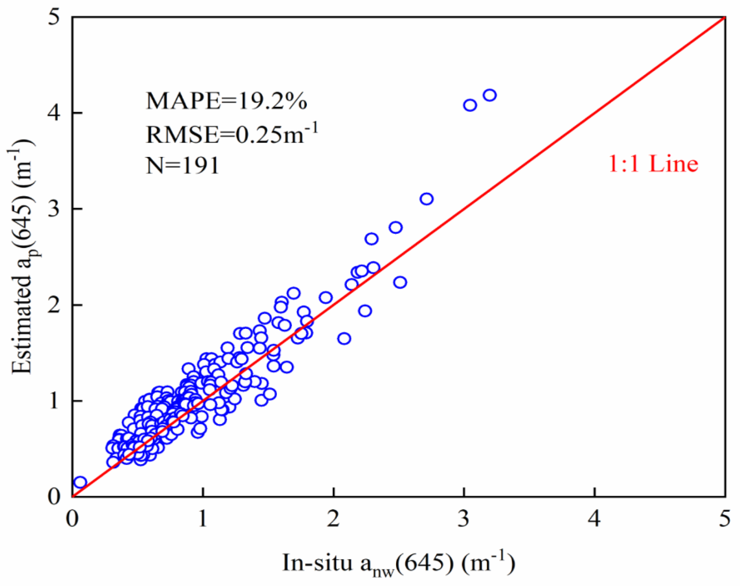
Finally, the nonwater absorption at 645 nm (anw(645)) can be deduced using step 6 of Table 1. According to the in-situ data, the absorption of CDOM at 645 nm (acodm(645)) was found to account for only 7.2% of ap(645). In other words, compared to ap(645), acodm(645) was so small that it could be ignored, so ap(645) was approximately equal to anw(645). The scatterplot of in-situ anw(645) and derived ap(645) is shown in Figure 3. The performance was satisfactory with MAPE of 19.2%, RMSE of 0.25 m−1, and validation points distributed approximately along the 1:1 line.
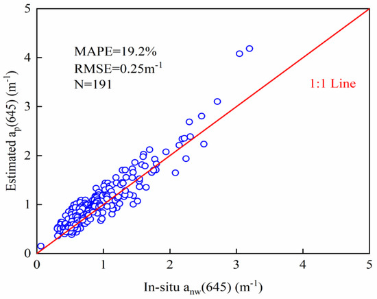
Figure 3.
Comparison of in-situ anw(645) and estimated ap(645).
2.6. Accuracy Assessment
In this study, the mean absolute percentage error (MAPE) and root mean square error (RMSE) were used to quantitatively evaluate the accuracy of the TSI estimation algorithm. The MAPE and RMSE were defined as Equations (8) and (9), respectively:
where Xobs,i is the measured TSI data, Xima,i is the inversion TSI data, and n is the number of samples.
3. Results
3.1. The Development of the TSI Estimation Algorithm
In this study, the particle absorption at 645 nm (ap(645)) was used to estimate the lake eutrophic state due to the stronger correlation between ap(645) and the TSI. Therefore, 2/3 of the total samples (N = 191) are used to develop the relationship between the TSI and ap(645), and the remaining 1/3 of the total samples (N = 95) are applied to the algorithm validation. Five mathematical function types (linear, logarithmic, exponential, power, and quadratic) were examined to establish the relationship between the TSI and ap(645) with the quadratic function having the best performance by having the highest determination coefficient. The TSI estimation algorithm based on ap(645) is described by Equation (10) with results illustrated in Figure 4.
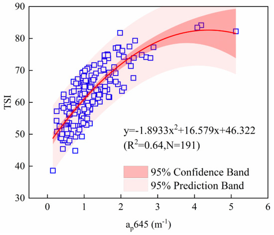
Figure 4.
Relationship between measured TSI and absorption coefficient of particulate matter at 645 nm.
3.2. The Accuracy Evaluation of the TSI Estimating Algorithm
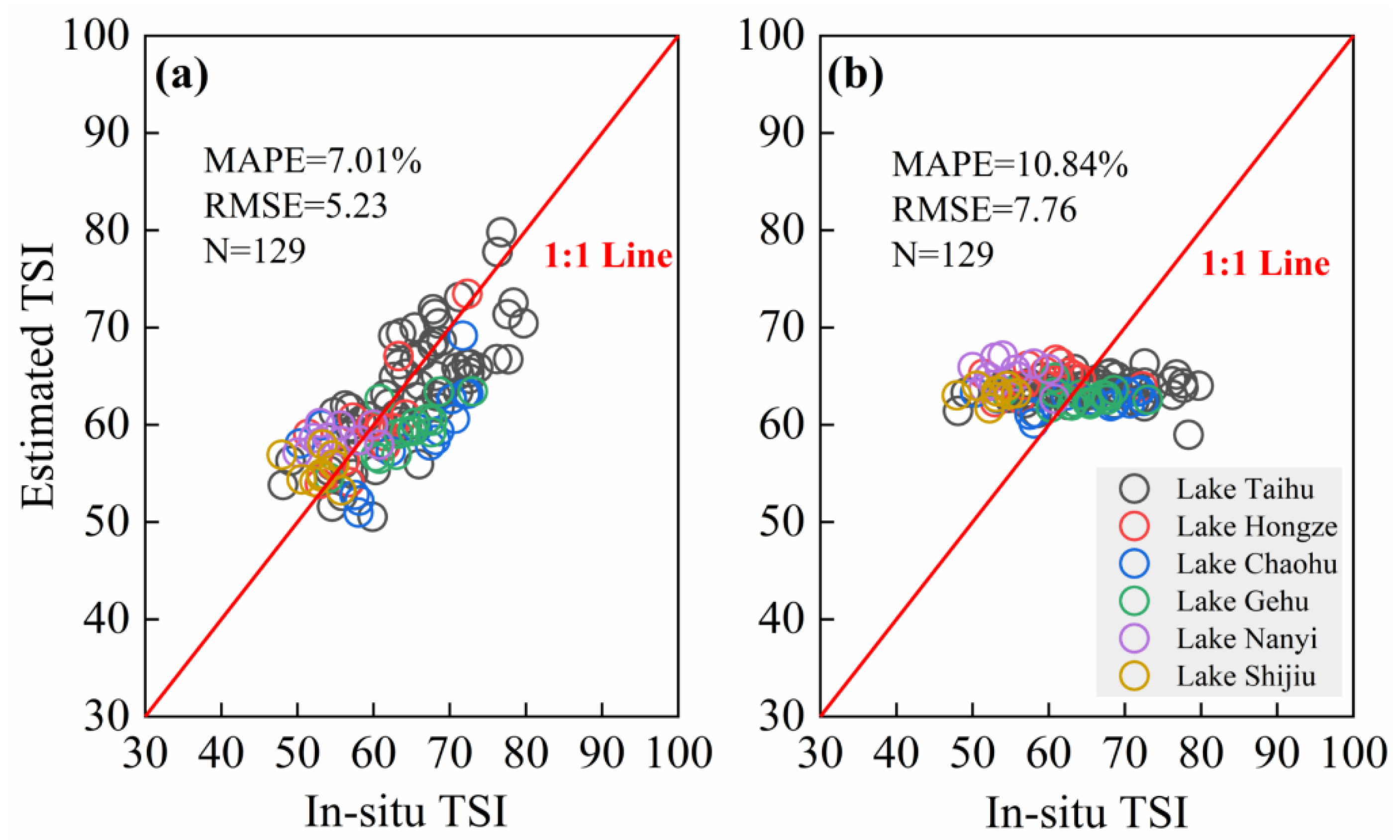
An independent validation dataset including 129 sampling data points was used to evaluate the proposed algorithm. Ninety five samples were from Lake Taihu, Lake Chaohu, and Lake Hongze with the other 34 samples from Lake Nanyi, Lake Shijiu, and Lake Gehu. The MAPE and RMSE were calculated using Equations (8) and (9) with values of 7.01% and 5.23, respectively. The scatter plot of the measured TSI and estimated TSI is shown in Figure 5a with values approximately distributed along the 1:1 line suggesting good agreement. The accuracy results demonstrated that the TSI estimation algorithm based on ap(645) has satisfactory performance.
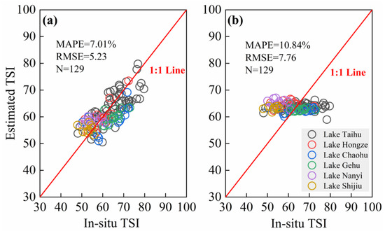
Figure 5.
(a) Comparison of in-situ TSI and estimated TSI based on our study; (b) Comparison of in-situ TSI and estimated TSI based on the algorithm of Shi.
Our proposed algorithm was also compared with the one proposed by Shi [6] that used at-w(440) to derive the TSI. The same validation dataset was also applied to calculate the MAPE and RMSE with values of 10.84% and 7.76, respectively. The scatter plot of estimated TSI using Shi’s algorithm and measured TSI is shown in Figure 5b. Shi’s algorithm performance is not very good in the YRD, especially in Lake Nanyi and Lake Shijiu. The MAPE and RMSE in Lake Nanyi were 19.39% and 11.06, and in Lake Shijiu they were 19.89% and 10.63, i.e., this method does not do well when applied in these two lakes. On the one hand, it is possible that Shi’s TSI calculations different from this paper. On the other hand, the poor skill may be that this method cannot be applied to lakes dominated by CDOM [6]. It can be clearly seen that the proposed algorithm of this study outperformed the older algorithm in the YRD.
3.3. Spatial Distribution of Lake Trophic State in the YRD
To obtain the spatial distribution of the TSI based on MODIS images, it was necessary to evaluate this algorithm’s applicability performance on real MODIS images. Therefore, a total of 134 sampling sites synchronized with the satellite overpass date were selected to evaluate the estimation algorithm accuracy. The scatterplot of in-situ and derived TSI from the MODIS image is shown in Figure 6. The performance of the proposed algorithm was satisfactory when applied to real MODIS images with MAPE of 9.29%, RMSE of 7.02, and validation points distributed approximately along the 1:1 line.
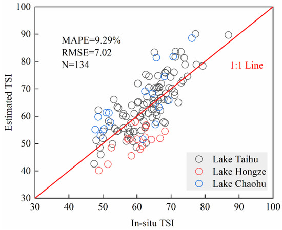
Figure 6.
Comparison of in-situ TSI and estimated TSI based on satellite ground synchronous points.
Therefore, the proposed algorithm could be used to obtain the long-term distribution pattern of the TSI in the YRD from 2002 to 2020, which provides reliable information for the study of the temporal and spatial changes in the TSI of lakes in the YRD.
Based on MODIS Aqua remote sensing images from 2002 to 2020, the spatial distribution characteristics of the TSI in the YRD are intensively analyzed and shown in Figure 7. The four subplots in Figure 7 represent the spatial distribution characteristics of different seasons and it can be clearly seen that the lake trophic state of the YRD changes significantly with the season. As seen in Figure 7, the overall lake TSI in the YRD is highest in summer (68.9 ± 7.52) and lowest in winter (65.75 ± 7.4), and there is no significant difference in spring and autumn. At the same time, it was found that 40.5% of lakes had a TSI that peaked in summer while the minimum value was observed in 71.4% of lakes in winter. In summer, many hypereutrophic levels can be observed in Lake Taihu, Lake Changdang, and Lake Chaohu. Previous studies have demonstrated that the highest Chla concentration is often found in both summer (June to August) and autumn (September to November) in Lake Taihu. In Lake Chaohu, the concentrations of Chla and TP are also the highest in summer. Therefore, the increase in these concentrations would lead to the most hypereutrophic state in the summer.
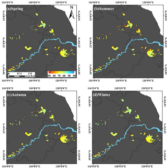
Figure 7.
The seasonal distribution pattern of the TSI in the YRD: (a) spring, (b) summer, (c) autumn, and (d) winter.
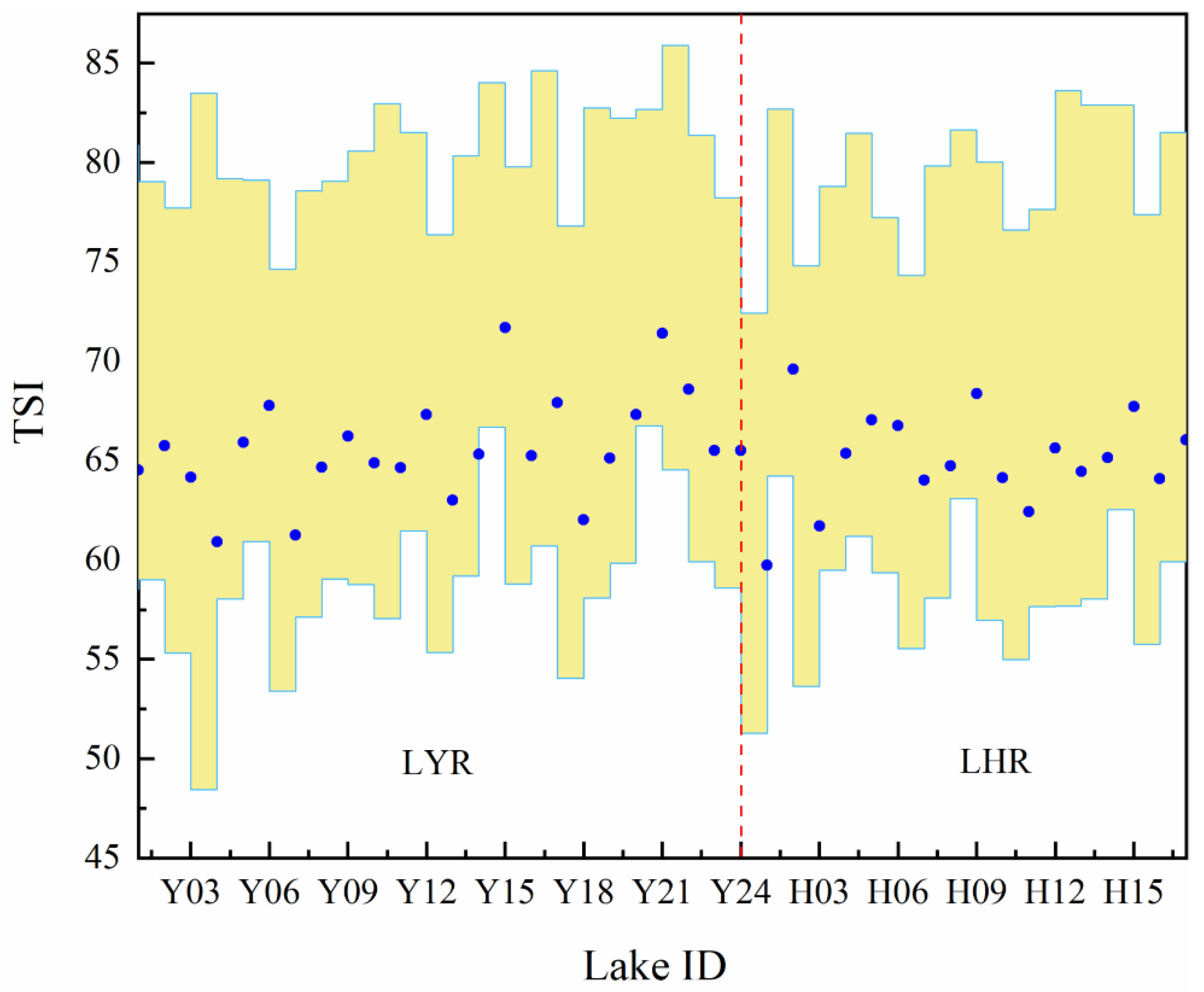
To further analyze the spatial differences of lakes in the YRD, the TSI mean value of all lakes in the YRD is illustrated in Figure 8. The TSI values showed that the lake trophic state in the YRD was moderately eutrophic. Comparing the lake trophic state of the LHR and LYR, there are 16 lakes with a state of moderate eutrophication and 2 lakes with a hypereutrophic state distributed in the LHR, and 22 moderate eutrophic lakes, and 1 mild eutrophic lake located in the LYR. Overall, the eutrophication of lakes in the LYR is more serious than that in the LHR. Figure 8 shows that compared to LHR, LYR has more lakes with higher TSI values, indicating that the eutrophication of LYR is more serious. Regarding individual lakes, Lake Gehu and Lake Changdang in the LYR have the highest average TSI, with a value of 71. Obviously, both lakes belong to the hypereutrophic level. In contrast, the lowest average TSI value was observed in Anfengtang Lake, which has a mild eutrophic state.
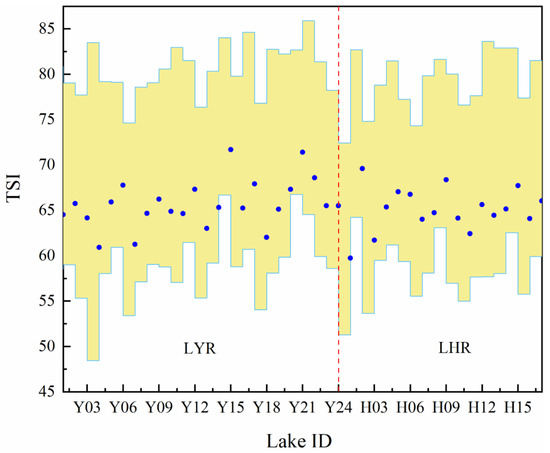
Figure 8.
Statistics of the mean TSI values of all lakes in the YRD. (The yellow bar represented the distribution range of the lake TSI in the YRD; the blue dot represented the average TSI of each lake; the red line was used to distinguish the lake groups belonging to LYR and LHR).
3.4. Temporal Changing Characteristics of the Lake Trophic State in the YRD
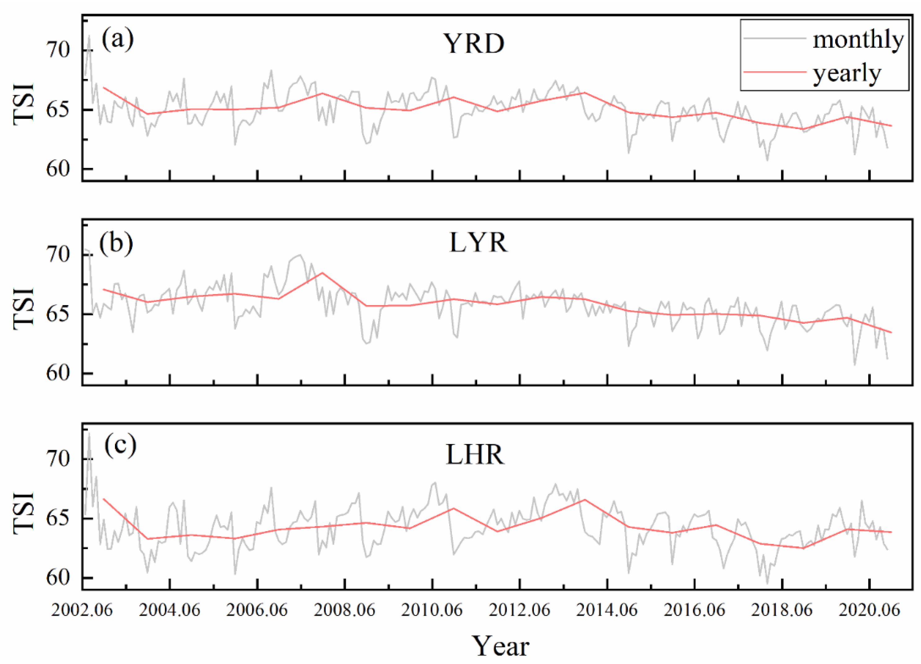
Annual and monthly changes in the average TSI in the YRD from 2002 to 2020 are shown in Figure 9. Generally, the highest value of TSI of lakes in the YRD often appeared in June each year, the lowest value was often observed in December, and the general change in TSI within the year was first to rise and then to fall.
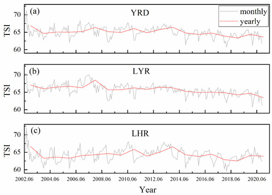
Figure 9.
Annual and monthly changes in the TSI average from 2002 to 2020: (a) YRD, (b) LYR, and (c) LHR.
Figure 9 shows that the average TSI value of lakes in the YRD showed a downward trend from 2002 to 2020, especially after 2013. A downward trend in LYR and LHR after 2013 was also observed. Furthermore, the TSI peak in the LYR appeared near 2007, which also made the TSI higher in 2007 in the YRD.
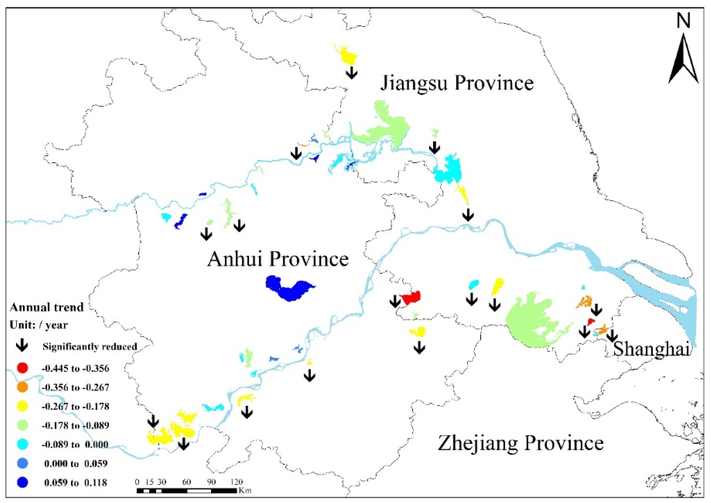
The interannual variation trend of the average TSI of each lake in the YRD is illustrated in Figure 10. Annual (year−1) TSI variation rate ranges of −0.445 to −0.356, −0.356 to −0.267, −0.267 to −0.178, −0.178 to −0.089, −0.089 to 0, 0 to 0.059, and 0.059 to 0.118 accounted for 4.8%, 7.1%, 19%, 21.4%, 26.2%, 9.5% and 9.5% of all lakes, respectively. Among them, Lake Shijiu exhibited the highest decrease rate with a value of −0.445 year−1, while Lake Chaohu exhibited the highest increase rate of 0.118 year−1. Significance analysis results demonstrated that 63.4% of lakes in the YRD experienced statistically significant decreasing trends (p < 0.05). Spatially, the lakes located in the eastern parts of the YRD all have a decreasing trend, while the lakes with decreasing trends in the northern, southwestern, and western subregions accounted for 69.2%, 80%, and 83.3% of all lakes, respectively.
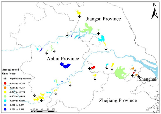
Figure 10.
Interannual variation trend of TSI of lakes in the YRD area observed by MODIS.
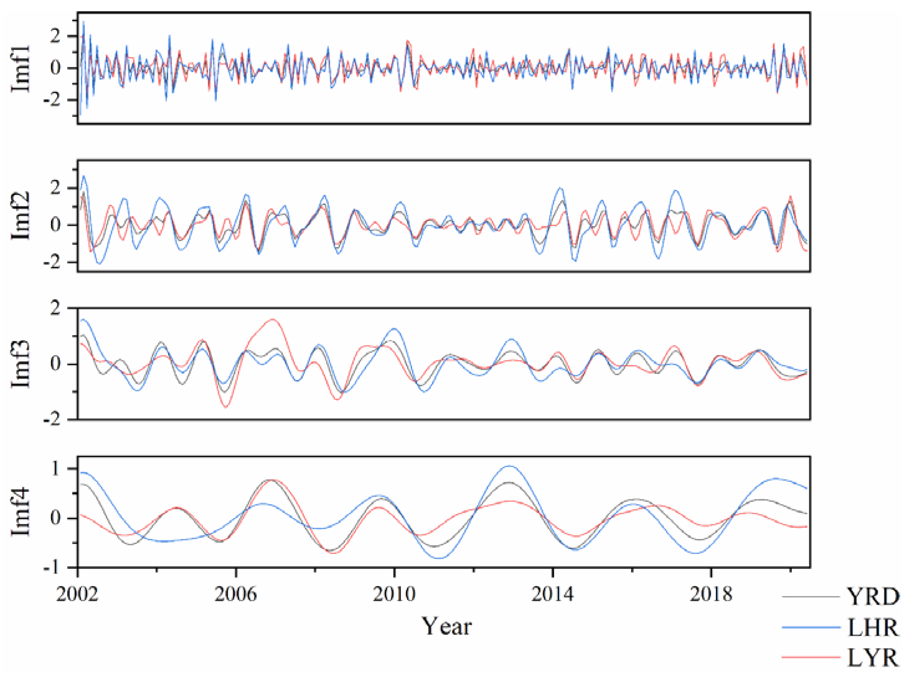
The EEMD method was also adopted to analyze the long-term change characteristics [26]. Figure 11 illustrates the seven intrinsic mode functions (IMFs) and residue decomposed from the monthly sequence data of the TSI (since the component variance contribution after IMF5 is so small, it is not shown). Table 2 shows the recorded periods and variance contribution of IMFs and the residues of the TSI in the YRD, LYR, and LHR. Table 2 shows that the period of the IMF1 component in the YRD is 2.2 months, which is a periodic signal that approximates the seasonal change. The period of its IMF2 component is 12 months, which is a marked interannual period. These two signal component contributions account for more than 50% of the total variance in the YRD region, so they are the main periodic variation contributors. In other words, the periodic change in the TSI in this region is mainly seasonal and interannual variation. Obvious TSI seasonal variation characteristics (IMF1, 3.85 ± 0.21 months) in the LYR and LHR can be clearly observed with variance contributions of 29.6% and 27.8%, respectively. The interannual period of TSI variation in the LYR and LHR is also obvious (IMF2, 12.25 ± 0.07 months) with variance contributions of 20.2% and 37.4%, respectively. These results show that seasonal and interannual variations in TSI values are the dominant trends in the YRD with only a small contribution caused by random factors.
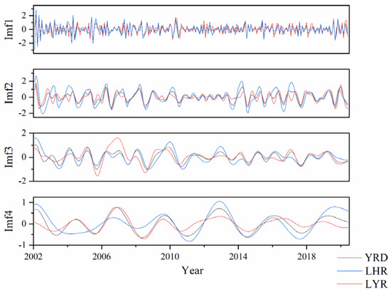
Figure 11.
IMFi of TSI in the YRD (gray line), LYR (red line), and LHR (blue line).
Table 2.
Periods and variance contribution of IMFs and the residues of TSI in the YRD, LYR, and LHR. (The unit of the period is a month, such that 3.7 months is an approximately seasonal period and 12.3 months is an approximately interannual periodicity. Residue indicates the general trends of TSI.)
4. Discussion
4.1. Why ap(645) Was Selected for TSI Retrievals
Recently, remote sensing methods have proven to be an effective way to assess the TSI level of lakes on a large scale. Most of these studies used Chla, SD, and TP to derive the TSI [4,6,14,15]. In this study, the correlation between the TSI and other relative parameters was intensively examined. Correlation coefficients between the TSI and ap(645), Chla, SD, and TP are shown in Figure 12. The Pearson’s r correlation coefficients between TSI and Chla, TP, and SD are 0.83, 0.72, and −0.45, respectively, while that between TSI and ap(645) is 0.86. Furthermore, ap(645) contains the absorbing information of the algae particulate (aph(645)) and the nonalgal particles (anap(645)), whereby aph(645) can reflect the concentration of Chla, and anap(645) can indicate the concentration of the total suspended matter so that the SD information of the lake could also be determined. Although ap(645) may not have a link with information on nutrients such as TP and TN, some studies have found that TP concentration is highly correlated with TSM in some lakes [12]. At the same time, a stronger correlation between ap(645) and TP was clearly observed in our data with a coefficient of 0.72, as seen in Figure 12, which was probably due to the correlation between TP and TSM. In summary, ap(645) can not only be used to characterize water color information but can also be an indicator of nutrient information. As a result, ap(645) was found to be highly correlated with TSI and can be an optimal proxy to reflect the trophic state of lakes.
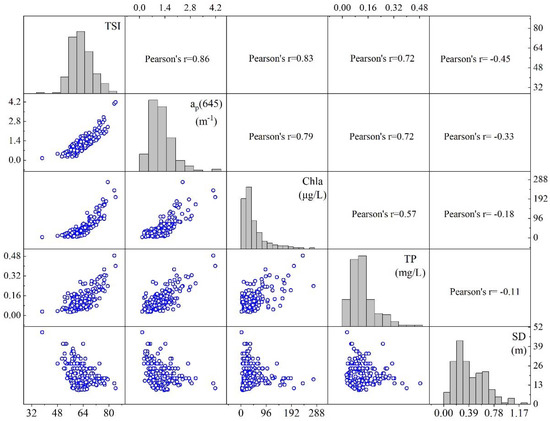
Figure 12.
Matrix scatter of correlation analysis between TSI, ap(645), Chla, SD, and TP.
SD and Chla are often adopted to indicate TSI by means of the relationship between them and TSI [4,11]. However, in optically complex inland waters, the information contained in only a single parameter is not enough, and the lake trophic state cannot be comprehensively evaluated. At the same time, some studies have tried to estimate the TSI by using a combination of parameters, such as SD, Chla, TP, etc., through remote sensing of each single parameter, though this approach will likely lead to the accumulation of remote sensing estimation errors from each retrieval [12].
The present study attempts to develop an algorithm to derive the TSI based on the particle absorption coefficient. ap(645), as an inherent optical property of inland waters, can be analytically derived based on remote sensing reflectance information. Furthermore, compared with other parameters, the R2 between the derived and in-situ ap(645) is the highest with a value of 0.74. Although ap(645) cannot contain all the information about the TSI-needed parameters, the ap(645) derived from the simplified QAA algorithm may cause deviations, which may cause uncertainty in TSI, it has more stable performance and higher accuracy than other algorithms. Therefore, by combining the QAA algorithm with the relationship between ap(645) and TSI, ap(645) was considered an optimal indicator for remote sensing of lake TSI in the YRD region based on MODIS data.
4.2. Evaluation of the Accuracy of the Simple and Operational Correction Method on MODIS Surface Reflectance Products
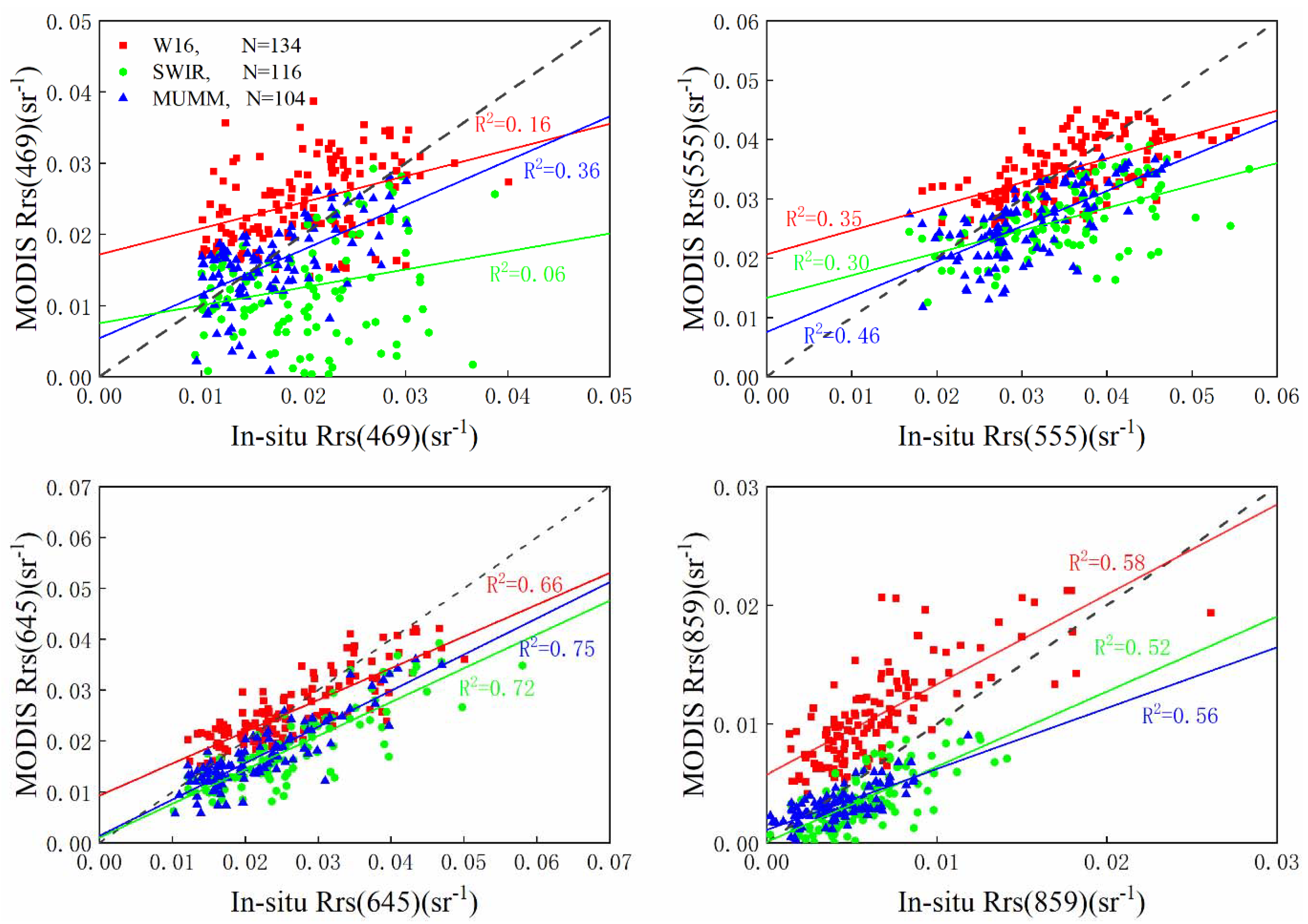
In this study, the simple and operational correction method (W16) was applied to atmospherically correct the MODIS surface reflectance product [27]. To evaluate the accuracy of atmospherically corrected MODIS surface reflectance, a total of 134 sampling points synchronized with satellite overpass date were used to validate the performance of W16, and the scatterplot of in situ remote sensing reflectance and remote sensing reflectance derived from the MODIS product is shown in Figure 13. Furthermore, SWIR and MUMM, two commonly used atmospheric correction methods for inland waters, were also applied to the MODIS product for an accuracy comparison with W16. The comparison result (Table 3) demonstrated that W16 can obtain 134 effective pixels, SWIR has 116 pixels, and MUMM has 104 pixels. The correlation coefficient (R2), RMSE, and MAPE were also calculated based on the synchronously measured remote sensing reflectance and derived remote sensing reflectance based on MODIS images using the different atmospheric correction methods. Detailed values are shown in Table 3. The R2 for W16 is 0.66 and 0.58 at 645 nm and 859 nm, respectively, which is close to the value obtained by using the MUMM and SWIR methods at these two bands. Table 3 shows that the RMSEs of the W16 method are 0.004967 sr−1 and 0.004974 sr−1 at 645 nm and 859 nm, respectively, and there is little difference among the three methods. According to the value of MAPE, W16 is only 15.46% at 645 nm, which is much lower than the other two methods; however, the MAPE at 859 nm is as high as 93.17%. This is due to the very low reflectivity values at this band [43].

Figure 13.
Comparison of three atmospheric correction methods.
Table 3.
Performance of three atmospheric correction methods.
Although the performance of W16 is not very good, W16 is recommended for large-scale, regional, or global lake monitoring due to its greater convenience and faster processing speed; in particular, it can be directly processed and obtained through the Google Earth Engine (GEE) platform. Compared with the other two methods, W16 has more effective available pixels, and there is no significant difference in the correction accuracy at 645 nm and 859 nm among the three methods. Therefore, the W16 method was selected to conduct atmospheric correction for this study. However, MODIS surface reflectance products have lower resolution, and fewer bands are available, so W16 can only be used when retrieving water quality parameters that are optically sensitive to the reflectance at 645 nm and 859 nm for large lakes (at least an area >10 km2). For other bands, a traditional atmospheric correction method, such as MUMM, is still recommended.
4.3. Analysis of the Driving Factors of Lake Trophic State Temporal Patterns in the YRD
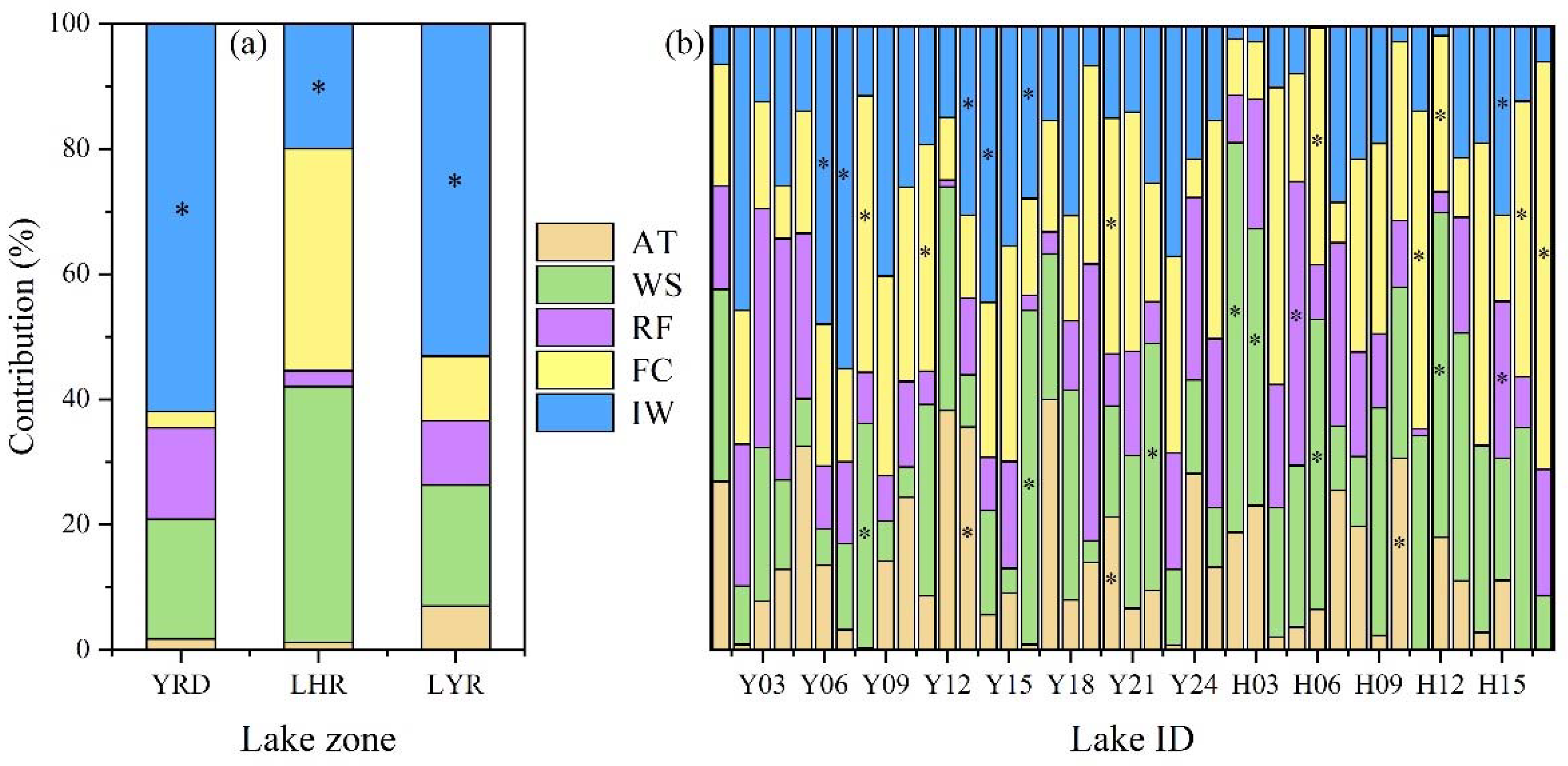
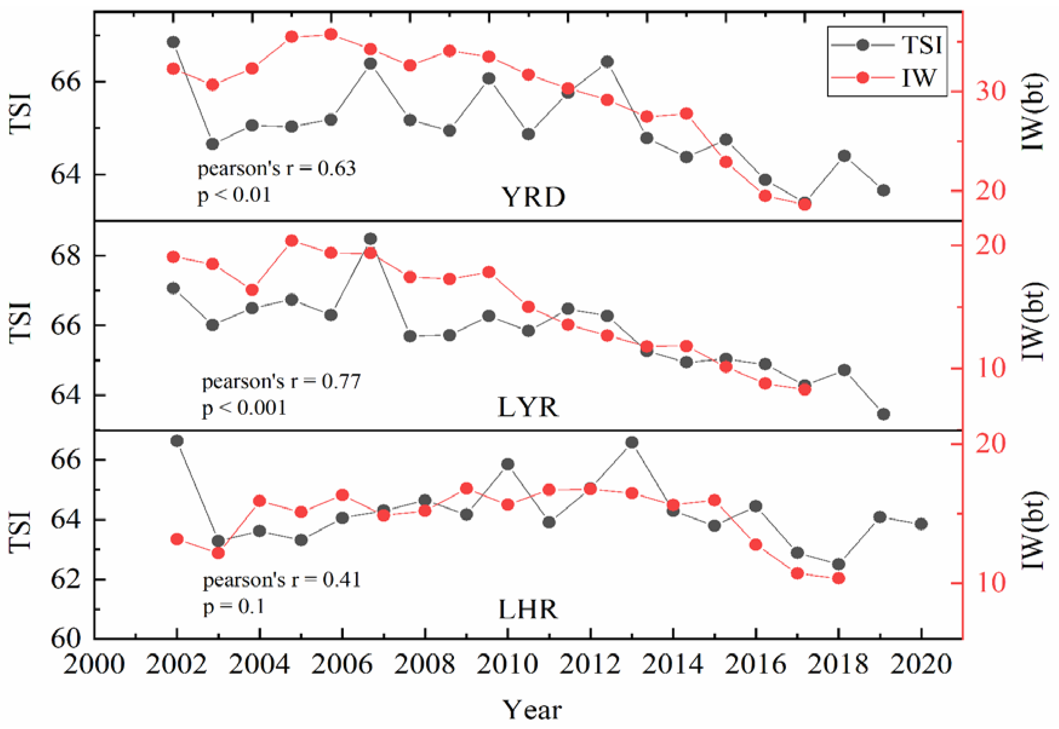
In this study, a multiple regression method was adopted to analyze the driving force for the variation of TSI in YRD. And five explanatory variables, air temperature (AT), wind speed (WS), rainfall (RF), fertilizer consumption (FC), and industrial wastewater (IW), were used to explain the long-term variation in TSI. The relative contribution ratios of different factors to the interannual changes in TSI of lakes in the YRD, LHR, and LYR are illustrated in Figure 14. Industrial wastewater clearly plays an important role in the TSI variation and explains 62% of the variation in the TSI in the YRD. The long-term variations of the TSI and industrial wastewater during the period from 2002 to 2020 are shown in Figure 15. In the subregions, industrial wastewater explains 20% and 53% of the variation in the TSI in the LHR and LYR, respectively (Figure 14a). Nutrient pollution in lakes is readily caused by large amounts of industrial wastewater discharge [5,33,34]. Nutrients such as phosphorus and nitrogen lead to the proliferation of cyanobacteria and other plankton [35]. This process consumes dissolved oxygen in lakes, resulting in the death of aquatic organisms and further harming water quality. Huang [5] also found that agriculture and residential areas were the main sources of wastewater resulting in algal blooms. In conclusion, industrial wastewater has a significant influence on the lake trophic state variation in the YRD.
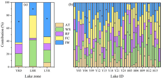
Figure 14.
(a) The relative contribution percentages of different factors to the interannual changes in the TSI of lakes in the YRD, LHR, and LYR; (b) the relative contributions of different factors to the interannual changes in the TSI of all lakes in the YRD. Here, AT, WS, RF, FC, and IW represent air temperature, wind speed, rainfall, fertilizer consumption, and industrial wastewater, respectively, and the symbol “*” represents p < 0.05.
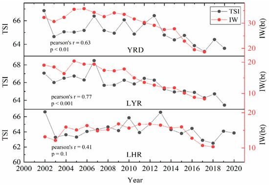
Figure 15.
Long-term variations in TSI and industrial wastewater in the YRD, LYR, and LHR from 2002 to 2020.
Air temperature, wind speed, rainfall, and fertilizer explained the remaining 38% of the lake trophic state changes in the YRD, of which 2% were explained by temperature, 19% by wind speed, 14% by rainfall, and 3% by fertilizer consumption. Although the amount of fertilizer consumption was relatively low, it explains 35% of the variation in the TSI in the LHR. This result demonstrated that the nitrogen and phosphorus contained in fertilizers could be the reason for lake trophic state variation through the nonpoint entry, such as the loss of nutrients from farmland [44]. Therefore, human activities have a great impact on the lake trophic state variation in the YRD.
In this study, the influence of meteorological factors on each lake’s trophic state variation was also investigated. From Figure 14b, climatic change is the main influencing factor of TSI variation in 21 lakes in the YRD. The results revealed that air temperature accounted for 23.8%, wind speed accounted for 47.6%, and rainfall accounted for 28.6%. It was found that wind speed has an impact on the trophic state variation in many lakes; for example, in Lake Baima, the wind speed could explain 63% of the variation in the TSI. Carrick [44] revealed that water-column phytoplankton chlorophyll correlated strongly with average daily wind speed in Lake Apopka because the wind and waves released soluble phosphorus on top of the sediments into the lake. In addition, the drop in air temperature could result in a decrease in Chla concentration and an increase in SD [45], which will ultimately lead to a decrease in TSI. Generally, climatic change will lead to variations in lake temperature, hydrological cycle, and hydrodynamic conditions [46]. It will also cause variations in agricultural production structure and agricultural land use, which would directly or indirectly affect the phosphorus cycle, thereby further affecting the lake ecosystem [47]. Under natural conditions, lakes will evolve slowly from an oligotrophic state to a eutrophic state [48]. The phenomenon of accelerated eutrophication processes in lakes can appear in a short time due to the artificial discharge of nutrient-containing industrial wastewater and domestic sewage [49], especially in the YRD, where human activities are intense.
5. Conclusions
In this study, a semi-analytical approach was finally developed to remotely assess the TSI in YRD lakes based on MODIS Aqua data. Particle absorption at 645 nm (ap(645)) can not only be used to characterize water color information but also be a good indicator of nutrient information. It was found that ap(645) has a good correlation with the required parameters for TSI calculation, such as Chla and SD. This proposed method will reduce transmission errors, and compared with the other often used approaches, the proposed method reduces the MAPE and RMSE by 3.83% and 5.4, respectively. Furthermore, this semi-analytical approach was successfully applied to MODIS images to obtain the spatial and temporal variation in the TSI in the YRD from 2002 to 2020.
Spatially, the average TSI of the lakes in the LYR was slightly higher than that in the LHR. The trophic state variation in lakes in the YRD had obvious interannual and seasonal fluctuations, with peaks in summer and valleys in winter. The overall trophic state reached a peak in 2007 Lakes with a downward trend of interannual variation accounted for 80% of the total lakes in the YRD. In addition, human activities were the main driving force influencing the lake trophic state during the study period. Industrial wastewater and fertilizer consumption in the farmland were found to be the two most important driving factors affecting the lake trophic state, explaining 65% of the variation in the TSI in the YRD. The contribution of climate factors to lake trophic state variation was relatively small. The approach of estimating TSI by remote sensing proposed in this study for larger lakes in the YRD provides an example for monitoring lake trophic state on a larger scale or even globally.
Author Contributions
Conceptualization, Y.B., F.G., and H.L. (Heng Lyu); Methodology, Y.B. and Y.Z.; Software, J.X.; Validation, Y.B., H.L. (Heng Lyu), and Y.L.; Formal Analysis, Y.B.; Investigation, S.N.; Resources, Y.Z.; Data Curation, J.X., H.L. (Huaiqing Liu); Writing-Original Draft Preparation, Y.B.; Writing-Review & Editing, Y.B.; Visualization, H.L. (Heng Lyu) and F.G.; Supervision, F.G. and Y.L. All authors have read and agreed to the published version of the manuscript.
Funding
This research is financially supported by the National Science Foundation of China grant (No. 41871234).
Institutional Review Board Statement
Not applicable.
Informed Consent Statement
Not applicable.
Data Availability Statement
Publicly available datasets were analyzed in this study. This data (China Meteorological Data Service Centre) can be found here: https://data.cma.cn/en (accessed on 14 July 2021).
Acknowledgments
We are grateful to the China Meteorological Data Service Centre who provides the meteorological data. Our thanks are extended to the remote sensing application graduate students from Nanjing Normal University, China, for their aid with the field work and lab analyses.
Conflicts of Interest
The authors declare no conflict of interest.
References
- Xiao, Y.; Ferreira, J.G.; Bricker, S.B.; Nunes, J.P.; Zhu, M.; Zhang, X. Trophic Assessment in Chinese coastal systems-review of methods and application to the Changjiang (Yangtze) Estuary and Jiaozhou Bay. Estuaries Coasts 2007, 30, 901–918. [Google Scholar] [CrossRef]
- Shi, K.; Zhang, Y.; Zhou, Y.; Liu, X.; Zhu, G.; Qin, B.; Gao, G. Long-term MODIS observations of cyanobacterial dynamics in Lake Taihu: Responses to nutrient enrichment and meteorological factors. Sci. Rep. 2017, 7. [Google Scholar] [CrossRef] [Green Version]
- Zhang, Y.; Ma, R.; Zhang, M.; Duan, H.; Loiselle, S.; Xu, J. Fourteen-Year Record (2000–2013) of the Spatial and Temporal Dynamics of Floating Algae Blooms in Lake Chaohu, Observed from Time Series of MODIS Images. Remote Sens. 2015, 7, 10523–10542. [Google Scholar] [CrossRef] [Green Version]
- Guan, Q.; Feng, L.; Hou, X.; Schurgers, G.; Zheng, Y.; Tang, J. Eutrophication changes in fifty large lakes on the Yangtze Plain of China derived from MERIS and OLCI observations. Remote Sens. Environ. 2020, 246. [Google Scholar] [CrossRef]
- Huang, C.; Wang, X.; Yang, H.; Li, Y.; Wang, Y.; Chen, X.; Xu, L. Satellite data regarding the eutrophication response to human activities in the plateau lake Dianchi in China from 1974 to 2009. Sci. Total Environ. 2014, 485-486, 1–11. [Google Scholar] [CrossRef] [PubMed]
- Shi, K.; Zhang, Y.; Song, K.; Liu, M.; Zhou, Y.; Zhang, Y.; Li, Y.; Zhu, G.; Qin, B. A semi-analytical approach for remote sensing of trophic state in inland waters: Bio-optical mechanism and application. Remote Sens. Environ. 2019, 232. [Google Scholar] [CrossRef]
- Smith, V.H.; Schindler, D.W. Eutrophication science: Where do we go from here? Trends Ecol. Evol. 2009, 24, 201–207. [Google Scholar] [CrossRef]
- Dodds, W.K. Trophic state, eutrophication and nutrient criteria in streams. Trends Ecol. Evol. 2007, 22, 669–676. [Google Scholar] [CrossRef]
- Chen, Q.; Huang, M.; Tang, X. Eutrophication assessment of seasonal urban lakes in China Yangtze River Basin using Landsat 8-derived Forel-Ule index: A six-year (2013–2018) observation. Sci. Total Environ. 2020, 745. [Google Scholar] [CrossRef] [PubMed]
- Wezernak, C.T.; Tanis, F.J.; Bajza, C.A. Trophic state analysis of inland lakes. Remote Sens. Environ. 1976, 5, 147–164. [Google Scholar] [CrossRef]
- Olmanson, L.G.; Bauer, M.E.; Brezonik, P.L. A 20-year Landsat water clarity census of Minnesota’s 10,000 lakes. Remote Sens. Environ. 2008, 112, 4086–4097. [Google Scholar] [CrossRef]
- Song, K.; Li, L.; Li, S.; Tedesco, L.; Hall, B.; Li, L. Hyperspectral Remote Sensing of Total Phosphorus (TP) in Three Central Indiana Water Supply Reservoirs. Water Air Soil Pollut. 2011, 223, 1481–1502. [Google Scholar] [CrossRef]
- Palmer, S.C.J.; Kutser, T.; Hunter, P.D. Remote sensing of inland waters: Challenges, progress and future directions. Remote Sens. Environ. 2015, 157, 1–8. [Google Scholar] [CrossRef] [Green Version]
- Wen, Z.; Song, K.; Liu, G.; Shang, Y.; Fang, C.; Du, J.; Lyu, L. Quantifying the trophic status of lakes using total light absorption of optically active components. Environ. Pollut. 2019, 245, 684–693. [Google Scholar] [CrossRef] [PubMed]
- Zhang, Y.; Zhou, Y.; Shi, K.; Qin, B.; Yao, X.; Zhang, Y. Optical properties and composition changes in chromophoric dissolved organic matter along trophic gradients: Implications for monitoring and assessing lake eutrophication. Water Res. 2018, 131, 255–263. [Google Scholar] [CrossRef]
- Shi, L.; Mao, Z.; Wu, J.; Liu, M.; Zhang, Y.; Wang, Z. Variations in Spectral Absorption Properties of Phytoplankton, Non-algal Particles and Chromophoric Dissolved Organic Matter in Lake Qiandaohu. Water 2017, 9, 352. [Google Scholar] [CrossRef] [Green Version]
- She, Q.; Peng, X.; Xu, Q.; Long, L.; Wei, N.; Liu, M.; Jia, W.; Zhou, T.; Han, J.; Xiang, W. Air quality and its response to satellite-derived urban form in the Yangtze River Delta, China. Ecol. Indic. 2017, 75, 297–306. [Google Scholar] [CrossRef]
- Duan, H.; Loiselle, S.A.; Zhu, L.; Feng, L.; Zhang, Y.; Ma, R. Distribution and incidence of algal blooms in Lake Taihu. Aquat. Sci. 2015, 77, 9–16. [Google Scholar] [CrossRef]
- Duan, H.; Ma, R.; Hu, C. Evaluation of remote sensing algorithms for cyanobacterial pigment retrievals during spring bloom formation in several lakes of East China. Remote Sens. Environ. 2012, 126, 126–135. [Google Scholar] [CrossRef]
- Cao, Z.; Duan, H.; Feng, L.; Ma, R.; Xue, K. Climate- and human-induced changes in suspended particulate matter over Lake Hongze on short and long timescales. Remote Sens. Environ. 2017, 192, 98–113. [Google Scholar] [CrossRef]
- Mobley, C.D. Estimation of the remote-sensing reflectance from above-surface measurements. Appl. Opt. 1999, 38. [Google Scholar] [CrossRef] [PubMed]
- Andersen, J. An ignition method for determination of total phosphorus in lake sediments. Water Res. 1976, 10, 329–331. [Google Scholar] [CrossRef]
- Tassan, S.; Ferrari, G.M. Proposal for the measurement of backward and total scattering by mineral particles suspended in water. Appl. Opt. 1995, 34. [Google Scholar] [CrossRef] [PubMed]
- Wang, S.; Li, J.; Zhang, B.; Lee, Z.; Spyrakos, E.; Feng, L.; Liu, C.; Zhao, H.; Wu, Y.; Zhu, L.; et al. Changes of water clarity in large lakes and reservoirs across China observed from long-term MODIS. Remote Sens. Environ. 2020, 247. [Google Scholar] [CrossRef]
- Huang, C.; Zhang, Y.; Huang, T.; Yang, H.; Li, Y.; Zhang, Z.; He, M.; Hu, Z.; Song, T.; Zhu, A.x. Long-term variation of phytoplankton biomass and physiology in Taihu lake as observed via MODIS satellite. Water Res. 2019, 153, 187–199. [Google Scholar] [CrossRef] [PubMed]
- Wang, M.; Son, S.; Shi, W. Evaluation of MODIS SWIR and NIR-SWIR atmospheric correction algorithms using SeaBASS data. Remote Sens. Environ. 2009, 113, 635–644. [Google Scholar] [CrossRef]
- Shenglei, W.; Junsheng, L.; Bing, Z.; Qian, S.; Fangfang, Z.; Zhaoyi, L. A simple correction method for the MODIS surface reflectance product over typical inland waters in China. Int. J. Remote Sens. 2016, 37, 6076–6096. [Google Scholar] [CrossRef]
- Wang, M. Estimation of ocean contribution at the MODIS near-infrared wavelengths along the east coast of the U.S.: Two case studies. Geophys. Res. Lett. 2005, 32. [Google Scholar] [CrossRef] [Green Version]
- Ruddick, K.G.; Ovidio, F.; Rijkeboer, M. Atmospheric correction of SeaWiFS imagery for turbid coastal and inland waters. Appl. Opt. 2000, 39. [Google Scholar] [CrossRef] [PubMed] [Green Version]
- Hu, C. A novel ocean color index to detect floating algae in the global oceans. Remote Sens. Environ. 2009, 113, 2118–2129. [Google Scholar] [CrossRef]
- Carlson, R.E. A trophic state index for lakes1. Limnol. Oceanogr. 1977, 22, 361–369. [Google Scholar] [CrossRef] [Green Version]
- Wu, Z.; Huang, N.E. Ensemble Empirical Mode Decomposition: A Noise-Assisted Data Analysis Method. Adv. Adapt. Data Anal. 2011, 1, 1–41. [Google Scholar] [CrossRef]
- Carpenter, S.R.; Caraco, N.F.; Correll, D.L.; Howarth, R.W.; Sharpley, A.N.; Smith, V.H. Nonpoint Pollution of Surface Waters with Phosphorus and Nitrogen. Ecol. Appl. 1998, 8, 559–568. [Google Scholar] [CrossRef]
- Le, C.; Zha, Y.; Li, Y.; Sun, D.; Lu, H.; Yin, B. Eutrophication of Lake Waters in China: Cost, Causes, and Control. Environ. Manag. 2010, 45, 662–668. [Google Scholar] [CrossRef]
- Timoshkin, O.A.; Moore, M.V.; Kulikova, N.N.; Tomberg, I.V.; Malnik, V.V.; Shimaraev, M.N.; Troitskaya, E.S.; Shirokaya, A.A.; Sinyukovich, V.N.; Zaitseva, E.P.; et al. Groundwater contamination by sewage causes benthic algal outbreaks in the littoral zone of Lake Baikal (East Siberia). J. Great Lakes Res. 2018, 44, 230–244. [Google Scholar] [CrossRef]
- Lee, Z.; Carder, K.L.; Arnone, R.A. Deriving inherent optical properties from water color: A multiband quasi-analytical algorithm for optically deep waters. Appl. Opt. 2002, 41. [Google Scholar] [CrossRef]
- Lyu, H.; Yang, Z.; Shi, L.; Li, Y.; Guo, H.; Zhong, S.; Miao, S.; Bi, S.; Li, Y. A Novel Algorithm to Estimate Phytoplankton Carbon Concentration in Inland Lakes Using Sentinel-3 OLCI Images. IEEE Trans. Geosci. Remote Sens. 2020, 58, 6512–6523. [Google Scholar] [CrossRef]
- Deng, R.; He, Y.; Qin, Y.; Chen, Q.; Chen, L. Pure water absorption coefficient measurement after eliminating the impact of suspended substance in spectrum from 400 nm to 900 nm. Yaogan Xuebao-J. Remote Sens. 2012, 16, 174–191. [Google Scholar]
- Ruddick, K.G.; De Cauwer, V.; Park, Y.-J.; Moore, G. Seaborne measurements of near infrared water-leaving reflectance: The similarity spectrum for turbid waters. Limnol. Oceanogr. 2006, 51, 1167–1179. [Google Scholar] [CrossRef] [Green Version]
- Sydor, M.; Gould, R.W.; Arnone, R.A.; Haltrin, V.I.; Goode, W. Uniqueness in remote sensing of the inherent optical properties of ocean water. Appl. Opt. 2004, 43. [Google Scholar] [CrossRef] [PubMed] [Green Version]
- Gitelson, A.A.; Dall’Olmo, G.; Moses, W.; Rundquist, D.C.; Barrow, T.; Fisher, T.R.; Gurlin, D.; Holz, J. A simple semi-analytical model for remote estimation of chlorophyll-a in turbid waters: Validation. Remote Sens. Environ. 2008, 112, 3582–3593. [Google Scholar] [CrossRef]
- Simis, S.G.H.; Ruiz-Verdú, A.; Domínguez-Gómez, J.A.; Peña-Martinez, R.; Peters, S.W.M.; Gons, H.J. Influence of phytoplankton pigment composition on remote sensing of cyanobacterial biomass. Remote Sens. Environ. 2007, 106, 414–427. [Google Scholar] [CrossRef]
- Shi, K.; Zhang, Y.; Zhu, G.; Liu, X.; Zhou, Y.; Xu, H.; Qin, B.; Liu, G.; Li, Y. Long-term remote monitoring of total suspended matter concentration in Lake Taihu using 250m MODIS-Aqua data. Remote Sens. Environ. 2015, 164, 43–56. [Google Scholar] [CrossRef]
- Carrick, H.J.; Aldridge, F.J.; Schelske, C.L. Wind Influences phytoplankton biomass and composition in a shallow, productive lake. Limnol. Oceanogr. 1993, 38, 1179–1192. [Google Scholar] [CrossRef]
- Wu, Z.; Zhang, Y.; Zhou, Y.; Liu, M.; Shi, K.; Yu, Z. Seasonal-Spatial Distribution and Long-Term Variation of Transparency in Xin’anjiang Reservoir: Implications for Reservoir Management. Int. J. Environ. Res. Public Health 2015, 12, 9492–9507. [Google Scholar] [CrossRef] [PubMed]
- Nazari-Sharabian, M.; Ahmad, S.; Karakouzian, M. Climate Change and Eutrophication: A Short Review. Eng. Technol. Appl. Sci. 2018, 8, 3668–3672. [Google Scholar] [CrossRef]
- Jeppesen, E.; Kronvang, B.; Meerhoff, M.; Søndergaard, M.; Hansen, K.M.; Andersen, H.E.; Lauridsen, T.L.; Liboriussen, L.; Beklioglu, M.; Özen, A.; et al. Climate Change Effects on Runoff, Catchment Phosphorus Loading and Lake Ecological State, and Potential Adaptations. J. Environ. Qual. 2009, 38, 1930–1941. [Google Scholar] [CrossRef] [PubMed]
- Lindeman, R.L. The Trophic-Dynamic Aspect of Ecology. Ecology 1942, 23, 399–417. [Google Scholar] [CrossRef]
- Bennett, E.M.; Carpenter, S.R.; Caraco, N.F. Human Impact on Erodable Phosphorus and Eutrophication: A Global Perspective. BioScience 2001, 51. [Google Scholar] [CrossRef]


Publisher’s Note: MDPI stays neutral with regard to jurisdictional claims in published maps and institutional affiliations. |
© 2021 by the authors. Licensee MDPI, Basel, Switzerland. This article is an open access article distributed under the terms and conditions of the Creative Commons Attribution (CC BY) license (https://creativecommons.org/licenses/by/4.0/).