Abstract
Atmospheric correction is a fundamental process of ocean color remote sensing to remove the atmospheric effect from the top-of-atmosphere. Generally, Near Infrared (NIR) based algorithms perform well for clear waters, while Ultraviolet (UV) based algorithms can obtain good results for turbid waters. However, the latter tends to produce noisy patterns for clear waters. An ideal and practical solution to deal with such a dilemma is to apply NIR- and UV-based algorithms for clear and turbid waters, respectively. We propose a novel atmospheric correction method that integrates the advantages of UV- and NIR-based atmospheric correction (AC) algorithms for coastal ocean color remote sensing. The new approach is called UV-NIR combined AC algorithm. The performance of the new algorithm is evaluated based on match-ups between GOCI images and the AERONET-OC dataset. The results show that the values of retrieved Rrs (Remote Sensing Reflectance) at visible bands agreed well with the in-situ observations. Compared with the SeaDAS (SeaWiFS Data Analysis System) standard NIR algorithm, the new AC algorithm can achieve better precision and provide more available data.
1. Introduction
The Geostationary Ocean Color Imager (GOCI), the world’s first geostationary ocean color spaceborne instrument, is onboard the Communication, Ocean, and Meteorological Satellite (COMS), which was launched in 2010 [1]. The GOCI offers moderate spatial resolution data (500 m × 500 m) for six visible bands and two infrared bands (centered around 412, 443, 490, 555, 660, 680, 745, and 865 nm) every hour during the daytime from 00:15 to 07:15 UTC. Its high-frequency sea-surface observation capability provides effective monitoring data for dynamic marine environment research. During the past 10 years, a large number of studies utilized the GOCI data for monitoring short-term coastal ocean phenomena, including suspended sediment dynamics [2,3,4,5], red tides [6,7], and tidal variability [8,9,10].
The effective use of the GOCI data depends on the atmospheric correction (AC) algorithm and ocean color information acquisition capabilities of the GOCI data [11]. The process of removing the influence of the atmosphere from the radiation signal received by the sensor is called AC [12]. In the AC process, the dominant contribution of the Rayleigh scattering can be accurately computed using a radiative transfer model with the inputs of solar-sensor geometries, atmospheric pressure, and surface wind speed, without using the remotely sensed data [13,14,15]. The difficulty of the AC is how to determine the type of aerosols and eliminate the scattering and absorption contribution of aerosols because of their unique optics and their temporal and spatial changes [16,17,18].
The widely used AC algorithm developed by Gordon and Wang [12] assumes that the reflectance from water is zero in the NIR (Near Infrared) band when estimating the aerosol scattering ratio (ε) [12,19]. The algorithm selects the closest aerosol model from candidate aerosol models, based on ε, and then extrapolates aerosol reflectance from NIR band to visible band [20,21]. This algorithm has given good results in the open ocean. However, in turbid coastal water, the reflectance from water in the NIR band is no longer zero, and the hypothesis of NIR “dark pixel” is no longer applicable. To overcome this problem, various AC algorithms use an iterative optimization scheme to separate water and aerosol reflectance in the NIR [22,23,24,25]. However, these iterative schemes result in biased estimations in ocean color products for the complex turbid waters [26,27]. To address this issue, Wang and Shi [28] proposed a NIR-SWIR (NIR-Short Wave Infrared) combined algorithm for AC of MODIS images. This method takes advantage of much stronger water absorption for the SWIR wavelengths and uses a turbidity index to apply a NIR-based algorithm for clear waters and a SWIR-based algorithm for turbid waters [29]. However, most current ocean color remote sensors, such as the Sea-viewing Wide Field-of-View Sensor (SeaWiFS), Medium Resolution Imaging Spectrometer (MERIS), and GOCI, do not include SWIR bands, which limits the application of this method. He et al. [30] proposed an AC algorithm based on the assumption of UV (Ultraviolet) “dark pixel” (UV-AC). The UV-AC algorithm produces good corrections for turbid waters.
The AC algorithms have advantages and disadvantages. There are four commonly used AC algorithms for the GOCI data process, including the UV-AC algorithm [30], KOSC standard AC (KOSC-STD) algorithm [31], NASA standard (NASA-STD) AC algorithm [23], and MUMM algorithm [32]. None of them can handle the AC for both clear and turbid waters perfectly. An ideal and practical solution to such a dilemma is to apply NIR- and UV-based algorithms for clear and turbid waters, respectively. The UV-AC method can be used to replace the SWIR method, the NIR algorithm for clean pixels, and the UV-AC method for turbid pixels.
In this study, we analyze the currently widely used GOCI image AC methods and use simulation datasets to evaluate the accuracy of three NIR-AC and one UV-AC algorithm. A novel AC method, called as UV-NIR combined AC algorithm, is proposed, which integrates the advantages of UV and NIR AC algorithms for GOCI coastal ocean color remote sensing. The new approach divides the applicable areas of the UV and NIR AC algorithms. After analyzing the application area of the UV and NIR AC algorithms and the characteristic cross-section remote sensing reflectance spectrum, a joint UV and NIR AC algorithm is constructed. Moreover, it is performed on the GOCI images of the Bohai Sea and the East China Sea, which contain both clear and turbid waters.
2. Materials and Methods
We use AC for retrieving water reflectance at the sea surface () by removing atmospheric reflectance. Ignoring the sunglint, whitecaps, and effects of bidirectional reflectance, the reflectance at the top of the atmosphere (TOA) () at wavelength can be described by [12]:
where is the TOA radiance, is the extraterrestrial solar irradiance, and is the solar zenith angle. is Rayleigh reflectance in the absence of aerosols, and is aerosol scattering reflectance. and are the upward and downward diffuse transmittances, respectively.
can be predicted given solar-sensor angular geometries and the air pressure at the surface through radiative transfer simulation with less than ~1% error [13,14,33]. The Rayleigh corrected reflectance () can be derived as follows:
To solve using Equation (3), the aerosol reflectance in the visible wavelengths is estimated first from the observed aerosol reflectance at the two NIR wavelengths or UV wavelengths based on the “dark pixel” assumption.
2.1. NASA-STD AC Algorithm
The NASA-STD AC algorithm uses a bio-optical model iterative process based on the Gordon and Wang method [12] for turbid water atmospheric correction. This method uses 80 types of aerosols built from the AERONET observations and vector radiative transfer code for the ocean-atmosphere system [21] and is currently the default AC algorithm of the SeaDAS software. It first uses the NIR band “dark pixel” method to obtain the water-leaving reflectance of the visible bands at 443 and 555 nm and then inputs the water-leaving reflectance at 443- and 555-nm bands into the bio-optical model (OBPG OC3 algorithm [34]) to determine chlorophyll concentration. Next, the backscattering coefficient at the 660-nm band is calculated according to the chlorophyll-a concentration, and the backscattering coefficient in the NIR band bbp(NIR) is calculated according to the relationship between 660 nm and the water backscattering coefficient in the NIR band [35]. The NIR water-leaving reflectance can then be calculated.
2.2. UV AC Algorithm
He et al. [30] studied a large number of in-situ water-leaving spectra of turbid estuary water bodies such as the Yangtze River, Mississippi River, and Orinoco River; they found that due to the high suspended solids concentration in the water body, the NIR radiation from water increased significantly. Meanwhile, due to the strong absorption of detritus, water-leaving radiance is significantly low in UV, which can be neglected [30]. Therefore, AC can be carried out through the UV band, that is, the UV algorithm. For the GOCI, He et al. [2] used 412 nm to estimate aerosol scattering. It first assumes the reflectance from water at 412 nm is 0, the aerosol scattering reflectance at 412 nm is equal to Rayleigh scattering correction reflectance (), and then estimates the aerosol scattering reflectance at 865 nm using the medium precision extrapolation model [12]. Next, it assumes that the 865 nm aerosol scattering reflectance is approximately the contribution of aerosol scattering in all bands (). The normalized water-leaving reflectance and remote sensing reflectance of water can be obtained by removing .
2.3. UV-NIR Jointed AC Algorithm
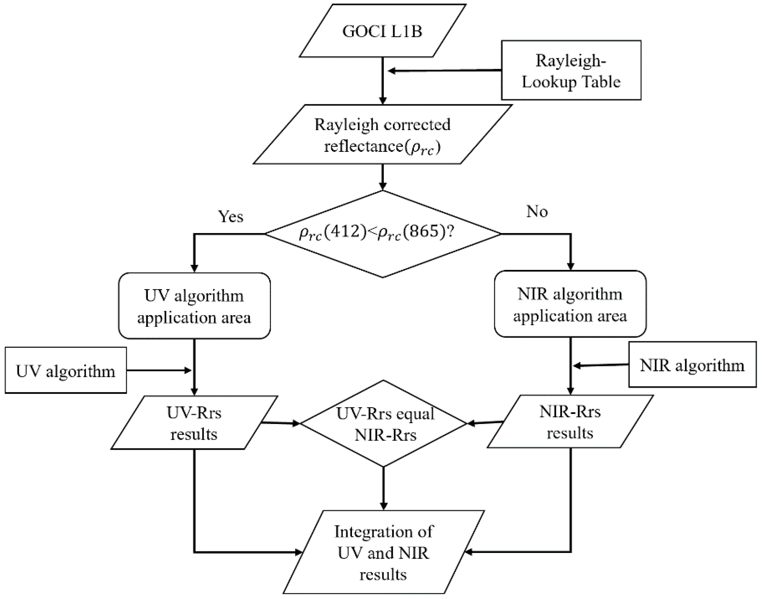
Through the analysis of the NASA-STD AC algorithm and specific implementation process of the UV AC (412 nm) algorithm, the starting point of the UV AC (412 nm) and NASA-STD AC is to assume that the water leaving reflectance of 412-nm or 865-nm band is zero; and the reflectance after Rayleigh correction is regarded as the contribution of aerosol scattering, which is then extrapolated to other bands’ aerosol scattering rates to complete AC. Therefore, the pixel can be divided into pixels processed by the UV or NIR AC algorithm according to the reflectance after Rayleigh correction at the 412-nm waveband and the 865-nm waveband. When , the UV AC (412 nm) algorithm should be used, otherwise, use the NIR AC algorithm. The flowchart of integrating UV and NIR AC algorithms is shown in Figure 1.
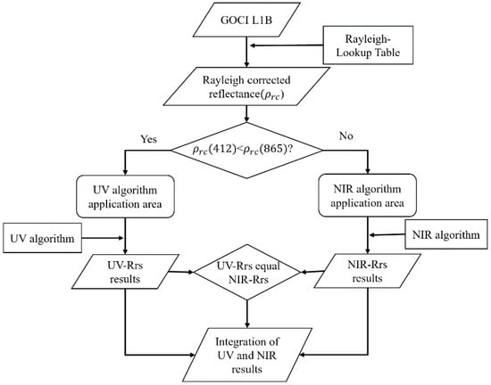
Figure 1.
The flowchart of integrating UV and NIR AC algorithms.
- (a)
- We use the GOCI Rayleigh scattering lookup table to perform Rayleigh scattering correction on the apparent reflectance of the TOA and obtain the Rayleigh scattering corrected reflectance for the 412-, 443-, 490-, 555-, 660-, 680-, 745-, and 865-nm bands.
- (b)
- According to the reflectance of 412- and 865-nm Rayleigh scattering correction, the applicable area of the AC algorithm is divided. The pixels of are the area of using the UV AC (412 nm) algorithm; the pixels of are the area of using the NIR AC algorithm.
- (c)
- The UV and NASA-STD AC algorithms are applied to the applicable areas of the UV and NIR AC algorithms obtained in step 2 to obtain the remote sensing reflectance ().
- (d)
- We utilize the UV AC (412 nm) algorithm for the pixels that have failed to use the NASA-STD AC algorithm and identify the pixels with the same remote sensing reflectance of the UV algorithm and NIR remote sensing reflectance; we use the UV AC (412 nm) remote sensing reflectance results on the shore side, and NASA-STD AC remote sensing reflectance results on the far shore side are accepted.
- (e)
- Finally, we integrate the remote sensing reflectance results of the UV algorithm application area, the NIR algorithm application area, and the transition area to obtain the whole AC result.
2.4. Simulated, GOCI and In-Suit Data
2.4.1. Simulated Top of Atmospheric (TOA) Reflectance
The NASA-STD, KOSC, and MUMM AC algorithms use NIR bands to estimate aerosol reflectance. We use simulated datasets to evaluate the accuracy of these three NIR AC algorithms and select the most accurate AC algorithm to combine with the UV AC (412 nm) algorithm. To generate a set of aerosol data containing broad aerosol properties, the Second Simulation of a Satellite Signal in the Solar Spectrum Vector Version 1.1 (6SV1.1) [36,37,38] was used to simulate aerosol reflectance. The input parameters are shown in Table 1. The solar and satellite geometry, zenith angle, and azimuth angle were extracted from the GOCI L2P file.

Table 1.
Parameters and values used in generating aerosol reflectance using 6SV1.1.
The simulated hyperspectral ocean color dataset provided by Nechad et al. [39] was used in this study because it consists of 5000 samples with a broad range of apparent optical properties (AOP) and inherent optical properties (IOP) ranging from 350 to 900 nm. The ranges of chlorophyll-a suspended sediment concentration and absorption coefficients (443 nm) of colored dissolved organic matter are 0~214.41 (mg/), 0~492.77 (g/), and 0~14.83 (1/m), respectively. The water-leaving reflectance spectra with zero solar and sensor zenith angles were used since they are equivalent to normalized water-leaving reflectance, and we do not need to consider the bidirectional reflectance distribution function effect. One simulated was selected for one simulated aerosol reflectance. The simulated Rayleigh-corrected reflectance was obtained by combining simulated aerosol and using . A total of 20,000 Rayleigh-corrected reflectance spectra were obtained.
2.4.2. GOCI and In-Suit Data
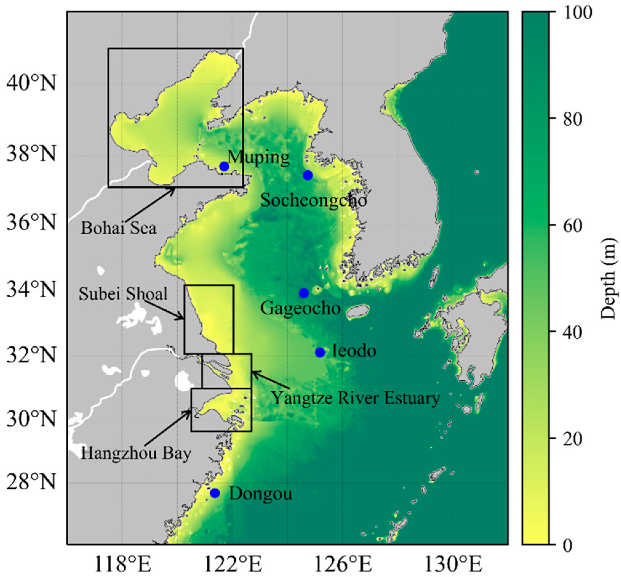
The spectra of in-situ Rrs were derived from Aerosol Robotic NETWORK-Ocean Color (AERONET-OC https://aeronet.gsfc.nasa.gov/new_web/ocean_color.html accessed date 4 October 2021) observations [40] and two Chinese ocean observation platforms (Station Muping and Station Dongou) locations are illustrated in Figure 2. The level 1B GOCI images collocated with in-situ samples were downloaded from the Korea Ocean Satellite Center (http://kosc.kiost.ac.kr/ accessed date 4 October 2021). Match-ups between the in-situ and GOCI-retrieved Rrs were selected based on locations and overpass times. The slight difference in the wavelength between the in-situ and satellite-retrieved values was ignored. First, 3 × 3 pixel boxes were extracted from the GOCI image centered on the measurement sites. Second, a coefficient of variation (CV, which is the standard deviation divided by mean values) was calculated for each band to account for spatial homogeneity of the pixels within each 3 × 3 box. Match-ups with CV values > 0.2 in 3 × 3 pixel boxes were excluded. Finally, the mean value of the remaining pixels was calculated. The in-suit data and the number of observations for each site are given in Table 2.

Figure 2.
Locations of five sampling stations and study area.
Table 2.
In-suit data location, description, and number of match-ups.
2.5. Performance Assessment
For quantitative performance assessment of the AC algorithms, different statistical matrices were used, namely, mean absolute percentage deviation (APD), root mean square error (RMSE), and the bias, as well as correlation coefficient ().
where Xi, Yi, and N are the in-situ value, retrieved value, and sample number, respectively.
3. Results
3.1. Evaluation of NIR Algorithms Using Simulated Data
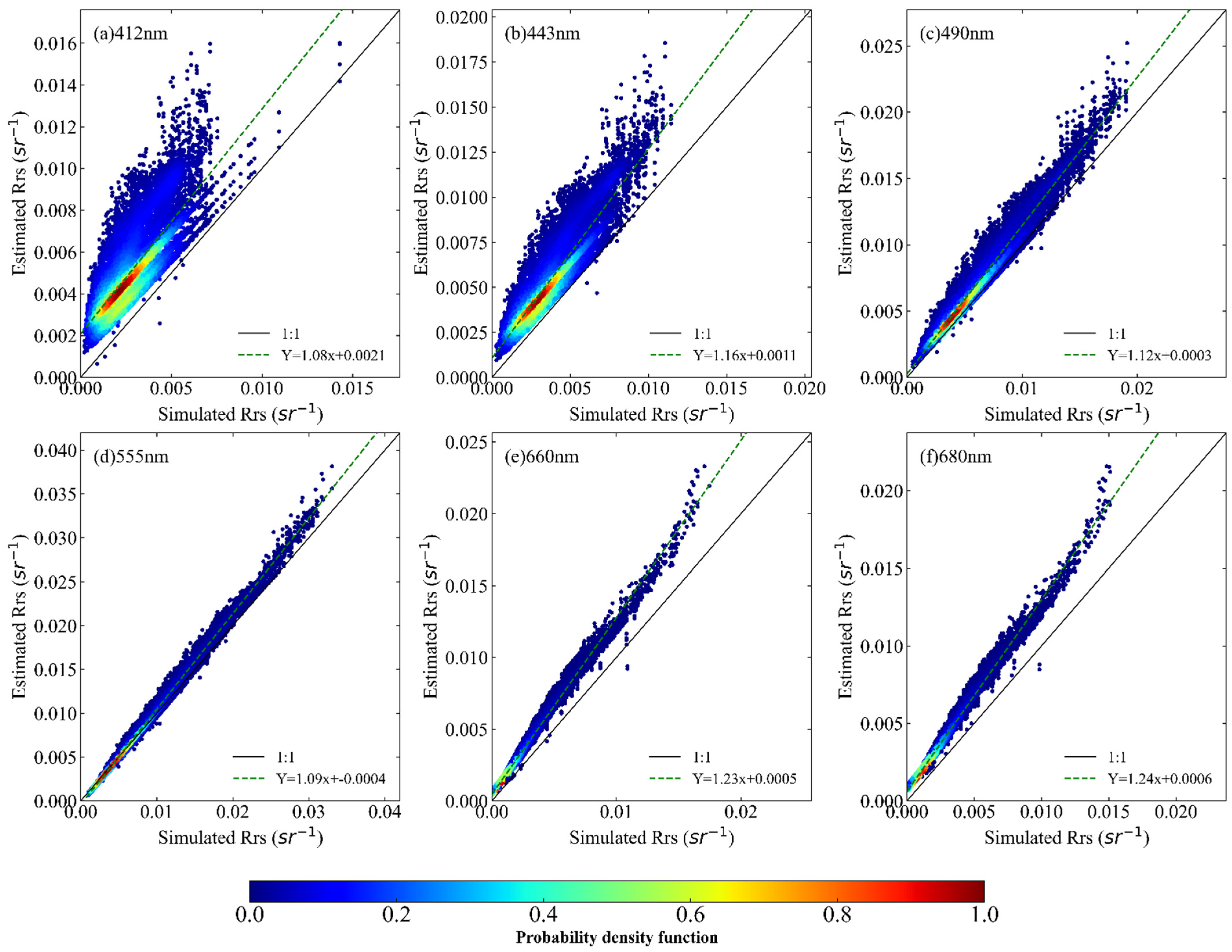
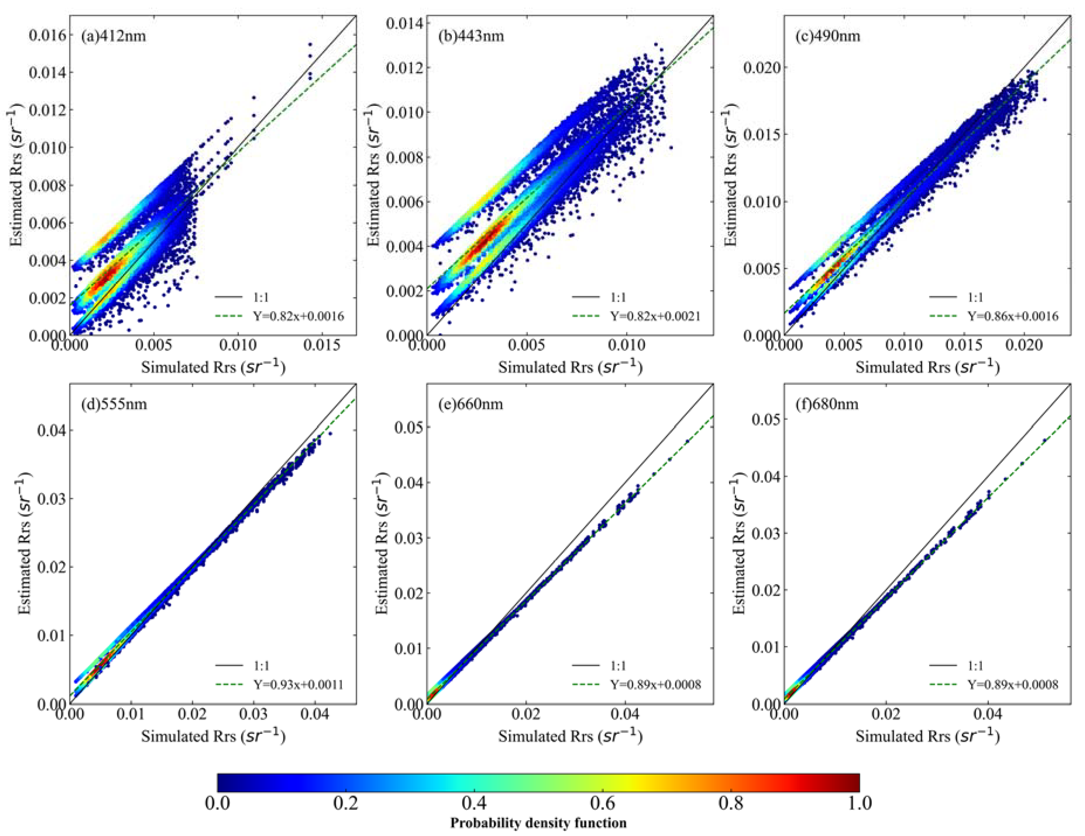
Figure 3, Figure 4 and Figure 5 and Table 3 compare AC results obtained by the KOSC algorithm, MUMM, and NASA-STD algorithm for the bands of 412, 443, 490, 555, 660, and 680 nm. The color in the figures represents the probability density of the scattered points; the redder the color, the greater the probability density. The solid black line is the 1:1 line, and the green dashed line is the fitting line of each band. It is clear that Rrs retrieval accuracy depends on the AC algorithm. The KOSC algorithm overestimates Rrs in all bands. The MUMM and NASA-STD algorithms overestimate Rrs in the 443 and 490 bands. Table 3 shows that the inversion values of the three NIR AC algorithms have a high correlation with the simulated remote sensing reflectance. In the 490-, 555-, 660-, and 680-nm bands, > 0.94; in the 443-nm band, the KOSC and NASA-STD algorithms have > 0.8, and the MUMM algorithm has = 0.74. The correlation in the 412-nm band is relatively low, and the of the KOSC, MUMM, and NASA-STD algorithms are 0.61, 0.54, and 0.61, respectively. The results of the three algorithms all show that at 490 and 555 nm, the remote sensing reflectance obtained is in good agreement with the simulated reflectance, and the APDs of the three algorithms in these two bands are between 12.14% and 20.94% and between 5.39% and 13.52%, respectively.
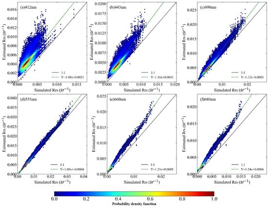
Figure 3.
Scatterplots of estimated vs. simulated remote sensing reflectance (Rrs) at 412, 443, 490, 555, and 660 nm, obtained using the KOSC algorithm. The solid is 1:1 line, and the dashed line is the regression line.

Figure 4.
Same as Figure 3, except using the MUMM algorithm.
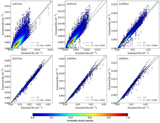
Figure 5.
Same as Figure 3, except using the NASA-STD algorithm.
Table 3.
Statistical results for the retrieved values of obtained with KOSC, MUMM, and NASA-STD algorithms.
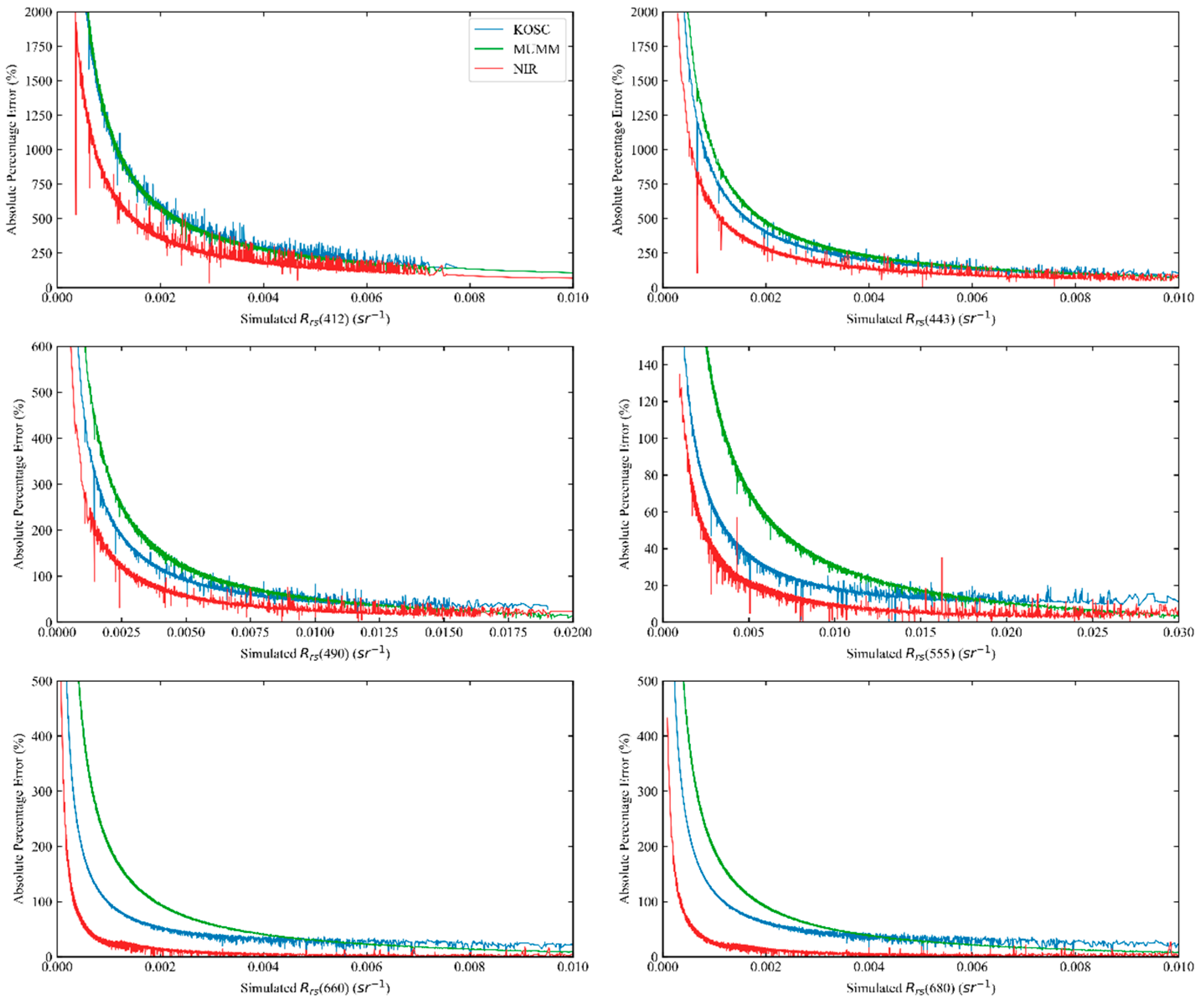
Figure 6 shows the APDs of Rrs retrieved using the KOSC, MUMM, and NASA-STD algorithms. The three algorithms all show the same pattern, and the APD decreases as the simulated Rrs increases. However, the APD of the NASA-STD algorithm is always the smallest. So, we choose the combination of NASA-STD and UV algorithms.
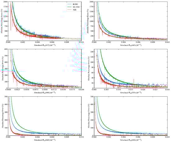
Figure 6.
Mean absolute percentage deviation (APD) of remote sensing reflectance (Rrs) retrieved from KOSC, MUMM, and NASA-STD algorithms as a function of simulated Rrs at 412, 443, 490, 555, 660, and 680 nm.
3.2. AC Algorithm Applicable Area Division
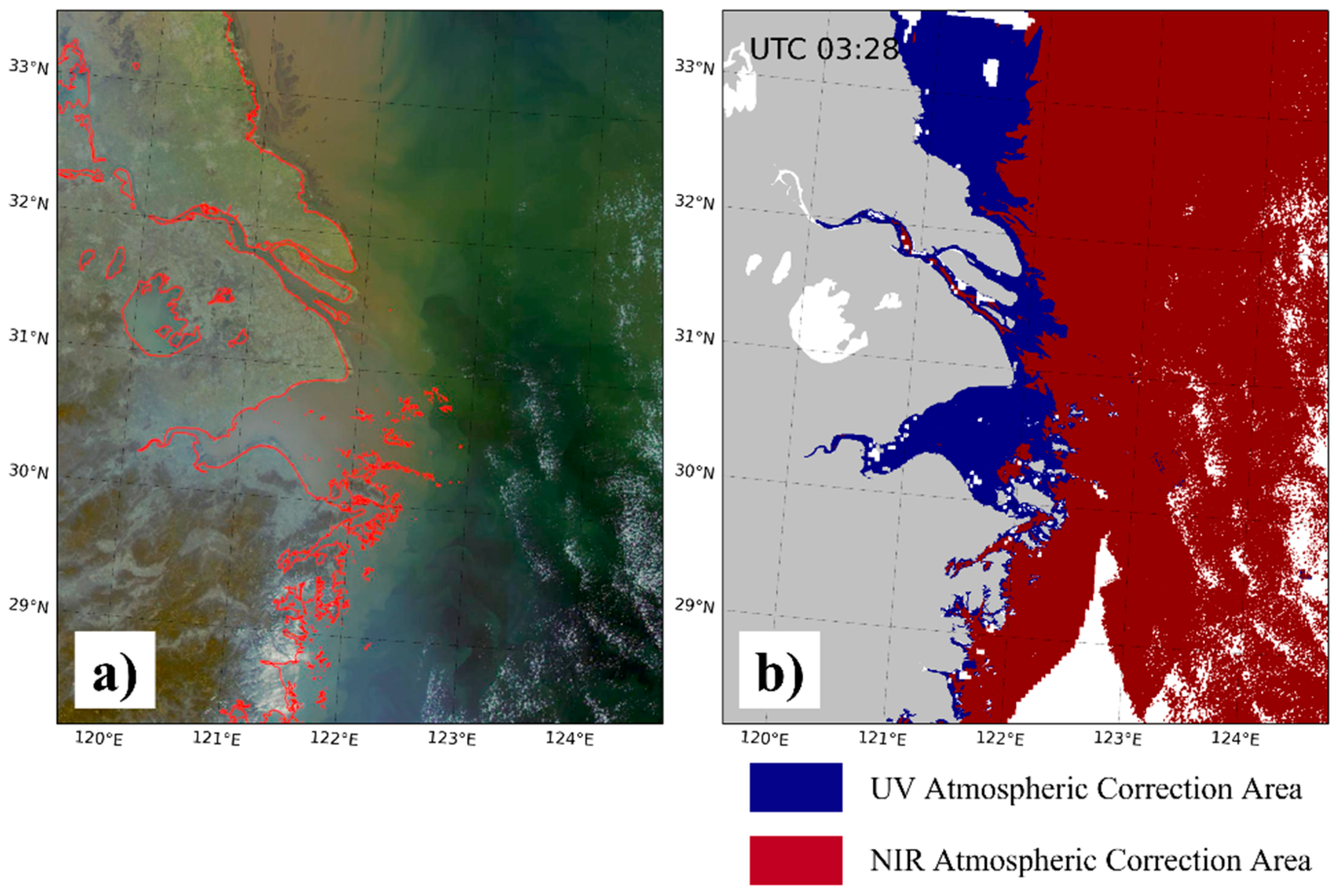
The division result is shown in Figure 7. The application area of the UV algorithm is mainly distributed in the offshore areas of Hangzhou Bay, the Yangtze River Estuary, and Subei Shoal. The application area of the NIR algorithm is mainly located offshore. In the clean water body far from the shore, most of the pixels on the image belong to the applicable area of the NIR algorithm.
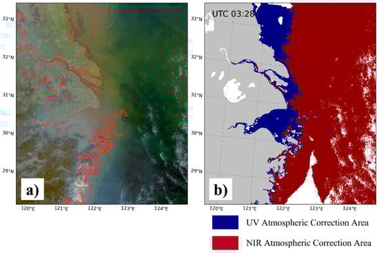
Figure 7.
Areas where the UV and NIR AC algorithms are applicable. The blank area on the image indicates cloud cover. (a) The true-color image of the GOCI sensor in the Yangtze River Estuary area at 11:30 on 1 March 2016. (b) Shows the application areas of the UV and NIR AC algorithms.
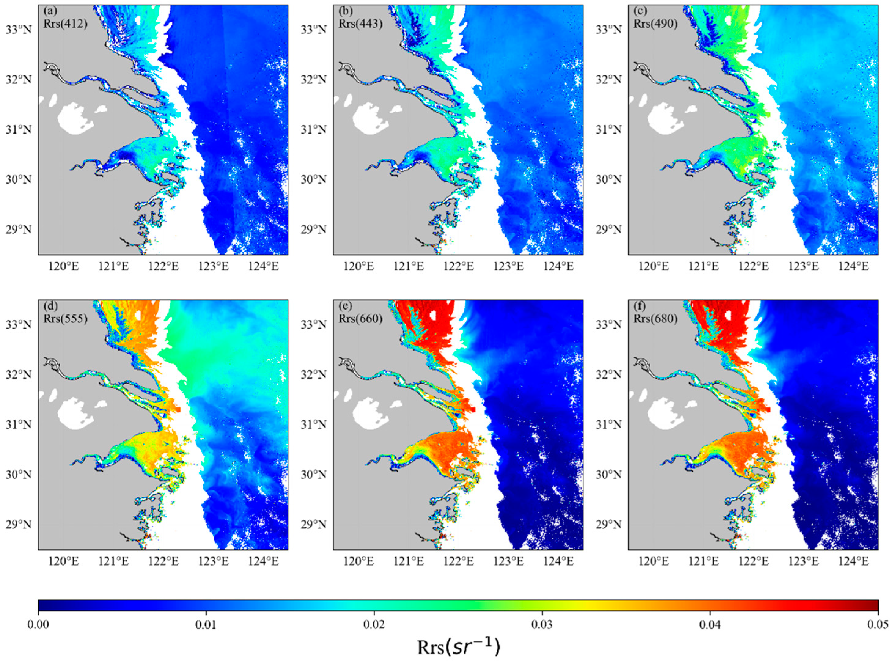
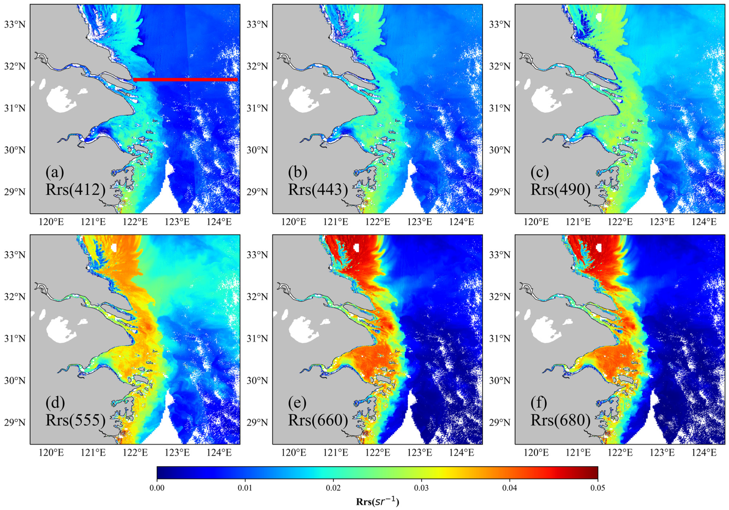
The UV AC (412 nm) algorithm and NASA-STD NIR AC algorithm are respectively applied to the areas shown in Figure 7, and the inverted remote sensing reflectance Rrs is shown in Figure 8. The UV algorithm shows good Rrs distribution in the 412–680 nm band. We use the NASA-STD NIR algorithm in the area where the NIR AC algorithm is applied. Good remote sensing reflectance results can be obtained in clear water bodies far offshore, but NASA-STD fails in the nearshore area (white area in Figure 8). Because the water there is still turbid, SeaDAS sets the flag of the pixels as turbid. Pixels cannot be processed using the NASA-STD NIR algorithm. We use the UV AC (412 nm) algorithm for processing these pixels.

Figure 8.
Atmospheric correction Rrs distributions (unit: ) at (a–f) 412, 443, 490, 555, 660, 680 nm on the Changjiang Estuary on 1 March 2016 by applying NASA-STD and UV algorithms to the applicable areas of NIR and UV. The black is the area where the NASA-STD algorithm fails, and the white is the cloud.
The UV algorithm can be used for effective inversion where the application area of the NIR algorithm cannot be retrieved, which increases the coverage area of the remote sensing reflectance products. However, this method has a clear dividing line in the area where the remote sensing reflectance of the UV and NIR algorithms intersect (Figure 9). The remote sensing reflectance jumps a lot there, which does not conform to the actual ocean water condition and is not continuous in space. It is necessary to smooth the transition from the UV algorithm to the NIR algorithm.
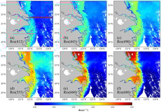
Figure 9.
UV-NIR atmospheric correction Rrs distributions (unit: ) at (a–f) 412, 443, 490, 555, 660, 680 nm on the Changjiang Estuary on 1 March 2016 by applying the UV algorithm to the NASA-STD algorithm failure area. The red line in panel (a) refers to the location and direction of the transect used in Figure 10.
3.3. Comparison of AC Results
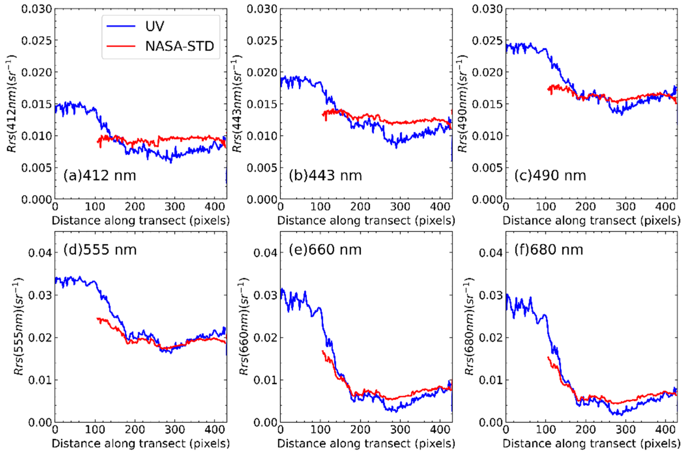
We also extracted the Rrs values for pixels along the red line in Figure 9. It covers the high-turbidity water body of the estuary and the offshore low-turbidity water body; their profiles are shown in Figure 10. A distance of 0 along the x-axis indicates the location is the closest to the coast. In general, values are low in the open ocean and high near the coast. At ~0–100 pixels along the transect, the NASA-STD algorithm is invalid. At the beginning of NASA-STD AC, the difference of results between the UV and NASA-STD algorithms is relatively large. Splicing here will cause a jump, so it is necessary to perform an algorithm conversion where the two are equal. At about 150 pixels, there is an intersection between the UV algorithm and NASA-STD NIR remote sensing reflectance curve, indicating that the remote sensing reflectance of the two is equal; after 150 pixels, the remote sensing reflectance of the UV AC (412 nm) algorithm continues to decrease; the NASA-STD NIR algorithm remote sensing changes smoothly in the 412–490 nm band, and gradually decreases in the 555–680 nm band, but the NIR algorithm remote sensing reflectance curve is always above the UV algorithm curve. The algorithm is switched there, the remote sensing reflectance (Rrs) transitions smoothly in space, and there will be no obvious dividing line.
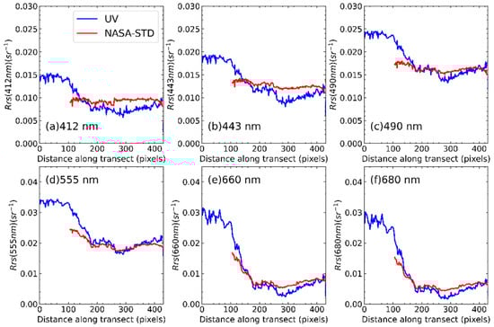
Figure 10.
Comparison of Rrs extracted from the pixel along the red arrow in Figure 9a at wavelengths of (a) 412, (b) 443, (c) 490, (d) 555, (e) 660, and (f) 680 nm. Zero on the x-axis indicates the location is the closest to the coast.
3.4. Algorithm Performance Evaluation Using Satellite Image
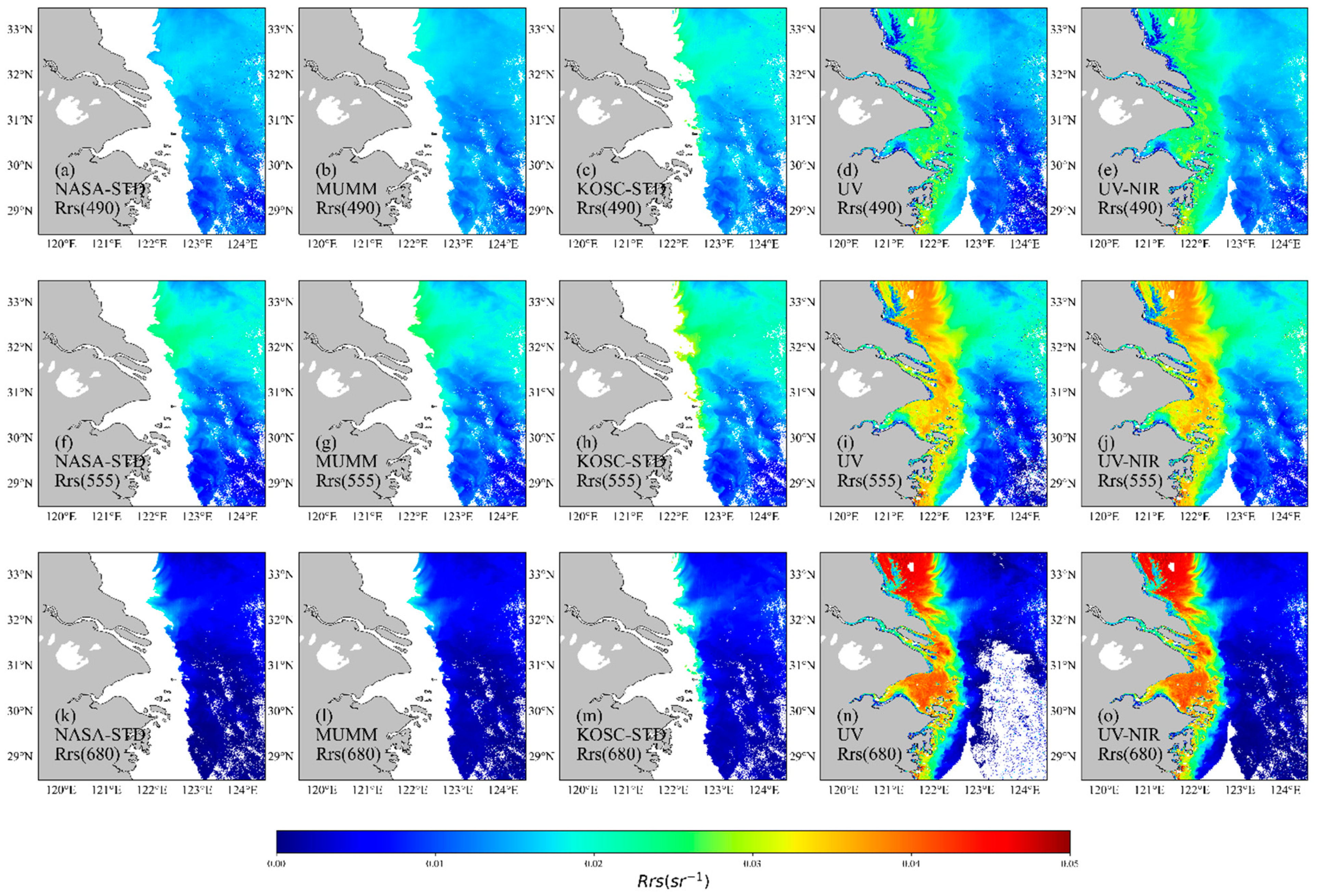
The results of the new algorithm are compared with those processed by NASA-STD, MUMM, KOSC-STD, and UV algorithms. Figure 11 and Figure 12 show that the NASA-STD AC algorithm does not have effective inversion values in the Changjiang Estuary and the Bohai Sea. The data loss is more serious in Hangzhou Bay and the Subei Shoal. The inversion effect is better in clean-water bodies far offshore. The UV AC (412 nm) algorithm can make up for the shortcoming of the NASA-STD algorithm, namely, not have an effective inversion value for turbid waters near the coast, but UV AC (412 nm) remote sensing reflectance appears a lot of negative values in the clean waters of the eastern Bohai Sea, which is displayed on the image after the negative value mask, and there are negative pixels in the 680-nm band in the East China Sea. In clean waters, there are no high concentrations of chlorophyll and yellow substances, and the light absorption of the water is weak. If the 412-nm band is regarded as a “dark pixel,” the Rayleigh-corrected reflectance of this band is regarded as aerosol reflectance. Aerosol scattering ratio extrapolation will overestimate the contribution of aerosol scattering on clean water, and the aerosols “flat” assumption is no longer applicable, so there will be a situation where the remote sensing reflectance of the clean-water body is negative, indicating that the UV AC (412 nm) algorithm does not apply to the clean-water body. The UV-NIR AC algorithm can effectively perform inversion in both near-shore turbid waters or clean ocean waters, indicating that the combined algorithm has the advantages of both NASA-STD NIR and UV algorithms and can effectively improve the coverage area of remote sensing reflectance.
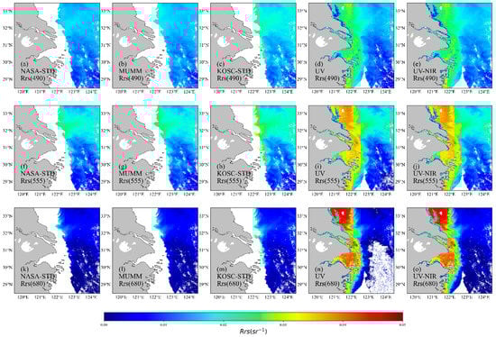
Figure 11.
Comparison of Rrs distributions (units: ) at (a–e) 490, (f–j) 555, and (k–o) 680 nm on the Changjiang Estuary on 1 March 2016, and processed by NASA-STD, MUMM, KOSC-STD, UV, and UV-NIR algorithms, respectively.
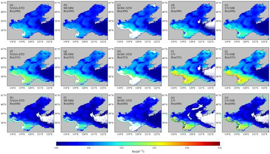
Figure 12.
Comparison of Rrs distributions (unit: ) at (a–e) 490, (f–j) 555, and (k–o) 680 nm in the Bohai Sea on 26 August 2016, and processed by NASA-STD, MUMM, KOSC-STD, UV, and UV-NIR algorithms, respectively.
3.5. Evaluation of UV-NIR AC Using In-Situ Data
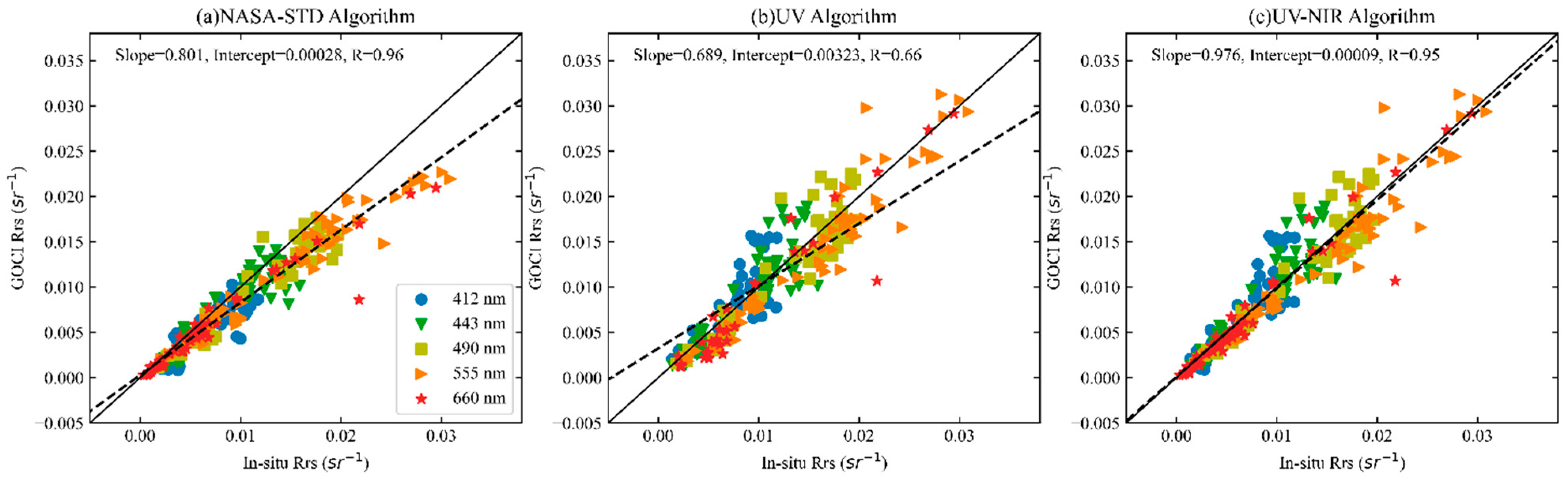
The slope in the overall Rrs match-ups for NASA-STD, UV, and UV-NIR algorithms are 0.801, 0.689, and 0.976, with an intercept of 0.00028, 0.00032, and 0.00009, respectively (Figure 13). Table 4 shows that the combined algorithm has the best performance, the RMSE is between 0.0017 and 0.0025, is between 0.77 and 0.94, and the relative error is between 12.95% and 23.37%. Among them, the relative error in the 443–660 nm band is less than 20%; and the average relative error appears in the 490-nm band, which is 12.95%; and the largest appears in the 412-nm band, which is 23.37%. The NASA-STD NIR algorithm significantly underestimates the remote sensing reflectance. Bias is between −0.0029 and −0.0011, and there is a small amount of negative values in the 412-nm band. The RMSE is between 0.0020 and 0.0036. The relative error is between 18.35% and 26.75%, and the average relative error is in the 412–555 nm band. The UV AC (412 nm) algorithm is slightly better than the NASA-STD AC algorithm; The 660 nm band error is the largest, with APD of 25.93% and a lot of negative values.

Figure 13.
Scatter plots of remote sensing reflectance inversion values and measured values using (a) NASA-STD algorithm, (b) UV algorithm, and (c) UV-NIR algorithms.
Table 4.
Statistical results of remote sensing reflectance inversion and measured values of three AC algorithms.
4. Conclusions
In this paper, the East China Sea is used as a research area, and the GOCI sensor data are selected to study AC methods. Aimed at current problems in the AC of coastal waters of the second type, a combined UV and NIR AC method is constructed to realize the AC of remote sensing images of turbid coastal waters.
According to the reflectance after Rayleigh scattering correction in the 412- and 865-nm bands, the image is divided into the applicable area of the UV algorithm and the applicable area of the NIR algorithm. Then, the UV and NIR AC algorithms are applied to their respective application areas. The results show that the applicable areas of the UV algorithm are mainly distributed in the offshore areas of Hangzhou Bay, the Yangtze River Estuary, and the Subei Shoal. The water body there is extremely turbid, and the concentration of suspended sediment is high. The applicable areas of the NIR algorithm are mainly distributed in clean-water bodies relatively far from the shore. The applicable area of AC is closely related to the temporal change of tide level. Applying the UV and NASA-STD NIR AC algorithms directly to the above areas will cause data discontinuities, and there will be obvious boundary lines on the image.
Based on the analysis of the applicable area of AC. A combined UV and NIR AC algorithm is proposed. Comparing the AC algorithm proposed in this paper with the UV and NASA-STD NIR algorithms, we find that the NASA-STD NIR algorithm has the worst accuracy (APD of 18.35–26.75%), and there is no effective inversion value in the coastal turbid water area. The accuracy of the UV AC (412 nm) algorithm is moderate (APD of 15.41–25.93%), and there are a small number of negative values in clean-water areas. The combined algorithm has the highest accuracy (APD of 13.86–23.37%), compared with the two individual algorithms: the average relative errors of 443–660 nm are decreased by 0.75–2.12%, 2.46–5.4%, 4.08–4.92%, and 2.35–6.4%, and the spatial coverage of data has also been greatly improved.
Author Contributions
Conceptualization, J.C. and F.Q.; methodology, F.Q.; software, F.Q. and Q.Z.; data analysis, F.Q. and Y.X.; investigation, J.C. and F.Q.; resources, Q.S., Z.M. and B.H.; writing F.Q. and J.C.; supervision, J.C.; project administration, J.C.; funding acquisition, J.C. All authors have read and agreed to the published version of the manuscript.
Funding
This research was funded by the National Key Research and Development Program of China (Grant No. 2016YFC1400903), NSFC-Zhejiang Joint Fund for the Integration of Industrialization and Informatization (Grant No. U1609202), Key Special Project for Introduced Talents Team of Southern Marine Science and Engineering Guangdong Laboratory (Guangzhou) (GML2019ZD0602), and National Natural Science Foundation of China (Grant Nos. 41376184 and 40976109).
Data Availability Statement
The authors thank the Korean Ocean Satellite Center (download URL:http://kosc.kiost.ac.kr/ accessed date 4 October 2021) for providing the GOCI data.
Conflicts of Interest
The authors declare no conflict of interest.
References
- Choi, J.-K.; Park, Y.J.; Ahn, J.H.; Lim, H.-S.; Eom, J.; Ryu, J.-H. GOCI, the World’s First Geostationary Ocean Color Observation Satellite, for the Monitoring of Temporal Variability in Coastal Water Turbidity. J. Geophys. Res. Ocean. 2012, 117, C09004. [Google Scholar] [CrossRef]
- He, X.; Bai, Y.; Pan, D.; Huang, N.; Dong, X.; Chen, J.; Chen, C.-T.A.; Cui, Q. Using Geostationary Satellite Ocean Color Data to Map the Diurnal Dynamics of Suspended Particulate Matter in Coastal Waters. Remote Sens. Environ. 2013, 133, 225–239. [Google Scholar] [CrossRef]
- Doxaran, D.; Lamquin, N.; Park, Y.-J.; Mazeran, C.; Ryu, J.-H.; Wang, M.; Poteau, A. Retrieval of the Seawater Reflectance for Suspended Solids Monitoring in the East China Sea Using MODIS, MERIS and GOCI Satellite Data. Remote Sens. Environ. 2014, 146, 36–48. [Google Scholar] [CrossRef]
- Chau, P.M.; Wang, C.-K.; Huang, A.-T. The Spatial-Temporal Distribution of GOCI-Derived Suspended Sediment in Taiwan Coastal Water Induced by Typhoon Soudelor. Remote Sens. 2021, 13, 194. [Google Scholar] [CrossRef]
- Du, Y.; Lin, H.; He, S.; Wang, D.; Wang, Y.P.; Zhang, J. Tide-Induced Variability and Mechanisms of Surface Suspended Sediment in the Zhoushan Archipelago along the Southeastern Coast of China Based on GOCI Data. Remote Sens. 2021, 13, 929. [Google Scholar] [CrossRef]
- Lou, X.; Hu, C. Diurnal Changes of a Harmful Algal Bloom in the East China Sea: Observations from GOCI. Remote Sens. Environ. 2014, 140, 562–572. [Google Scholar] [CrossRef]
- Lee, M.-S.; Park, K.-A.; Micheli, F. Derivation of Red Tide Index and Density Using Geostationary Ocean Color Imager (GOCI) Data. Remote Sens. 2021, 13, 298. [Google Scholar] [CrossRef]
- Hu, Z.; Wang, D.P.; Pan, D.; He, X.; Miyazawa, Y.; Bai, Y.; Wang, D.; Gong, F. Mapping Surface Tidal Currents and Changjiang Plume in the East China Sea from Geostationary Ocean Color Imager. J. Geophys. Res. Ocean. 2016, 121, 1563–1572. [Google Scholar] [CrossRef] [Green Version]
- Park, K.-A.; Lee, M.-S.; Park, J.-E.; Ullman, D.; Cornillon, P.C.; Park, Y.-J. Surface Currents from Hourly Variations of Suspended Particulate Matter from Geostationary Ocean Color Imager Data. Int. J. Remote Sens. 2018, 39, 1929–1949. [Google Scholar] [CrossRef] [Green Version]
- Chen, J.; Chen, J.; Cao, Z.; Shen, Y. Improving Surface Current Estimation From Geostationary Ocean Color Imager Using Tidal Ellipse and Angular Limitation. J. Geophys. Res. Ocean. 2019, 124, 4322–4333. [Google Scholar] [CrossRef]
- Wang, M.; Shi, W.; Jiang, L. Atmospheric Correction Using Near-Infrared Bands for Satellite Ocean Color Data Processing in the Turbid Western Pacific Region. Opt. Express 2012, 20, 741. [Google Scholar] [CrossRef]
- Gordon, H.R.; Wang, M. Retrieval of Water-Leaving Radiance and Aerosol Optical Thickness over the Oceans with SeaWiFS: A Preliminary Algorithm. Appl. Opt. 1994, 33, 443. [Google Scholar] [CrossRef] [PubMed]
- Gordon, H.R.; Wang, M. Surface-Roughness Considerations for Atmospheric Correction of Ocean Color Sensors 1: The Rayleigh-Scattering Component. Appl. Opt. 1992, 31, 4247. [Google Scholar] [CrossRef] [PubMed]
- Wang, M. The Rayleigh Lookup Tables for the SeaWiFS Data Processing: Accounting for the Effects of Ocean Surface Roughness. Int. J. Remote Sens. 2002, 23, 2693–2702. [Google Scholar] [CrossRef]
- Shanmugam, V.; Shanmugam, P.; He, X. New Algorithm for Computation of the Rayleigh-Scattering Radiance for Remote Sensing of Water Color from Space. Opt. Express 2019, 27, 30116. [Google Scholar] [CrossRef]
- Liu, G.; Li, Y.; Lyu, H.; Wang, S.; Du, C.; Huang, C. An Improved Land Target-Based Atmospheric Correction Method for Lake Taihu. IEEE J. Sel. Top. Appl. Earth Obs. Remote Sens. 2016, 9, 793–803. [Google Scholar] [CrossRef]
- Wang, M.; Jiang, L. Atmospheric Correction Using the Information From the Short Blue Band. IEEE Trans. Geosci. Remote Sens. 2018, 56, 6224–6237. [Google Scholar] [CrossRef]
- Pan, Y.; Shen, F.; Verhoef, W. An Improved Spectral Optimization Algorithm for Atmospheric Correction over Turbid Coastal Waters: A Case Study from the Changjiang (Yangtze) Estuary and the Adjacent Coast. Remote Sens. Environ. 2017, 191, 197–214. [Google Scholar] [CrossRef] [Green Version]
- Gordon, H.R. Removal of Atmospheric Effects from Satellite Imagery of the Oceans. Appl. Opt. 1978, 17, 1631. [Google Scholar] [CrossRef]
- Shettle, E.; Fenn, R. Models for the Aerosols of the Lower Atmosphere and the Effects of Humidity Variations on Their Optical Properties. Environ. Res. 1979, 94, 504. [Google Scholar]
- Ahmad, Z.; Franz, B.A.; McClain, C.R.; Kwiatkowska, E.J.; Werdell, J.; Shettle, E.P.; Holben, B.N. New Aerosol Models for the Retrieval of Aerosol Optical Thickness and Normalized Water-Leaving Radiances from the SeaWiFS and MODIS Sensors over Coastal Regions and Open Oceans. Appl. Opt. 2010, 49, 5545. [Google Scholar] [CrossRef]
- Mobley, C.D.; Werdell, J.; Franz, B.; Ahmad, Z.; Bailey, S. Atmospheric Correction for Satellite Ocean Color Radiometry. Tech. Rep. 2016, 85. [Google Scholar] [CrossRef]
- Bailey, S.W.; Franz, B.A.; Werdell, P.J. Estimation of Near-Infrared Water-Leaving Reflectance for Satellite Ocean Color Data Processing. Opt. Express 2010, 18, 7521. [Google Scholar] [CrossRef] [PubMed]
- Ahn, J.-H.; Park, Y.-J. Estimating Water Reflectance at Near-Infrared Wavelengths for Turbid Water Atmospheric Correction: A Preliminary Study for GOCI-II. Remote Sens. 2020, 12, 3791. [Google Scholar] [CrossRef]
- Xue, C.; Chen, S.; Lee, Z.; Hu, L.; Shi, X.; Lin, M.; Liu, J.; Ma, C.; Song, Q.; Zhang, T. Iterative Near-Infrared Atmospheric Correction Scheme for Global Coastal Waters. ISPRS J. Photogramm. Remote Sens. 2021, 179, 92–107. [Google Scholar] [CrossRef]
- Pahlevan, N.; Roger, J.-C.; Ahmad, Z. Revisiting Short-Wave-Infrared (SWIR) Bands for Atmospheric Correction in Coastal Waters. Opt. Express 2017, 25, 6015. [Google Scholar] [CrossRef] [PubMed]
- Goyens, C.; Jamet, C.; Schroeder, T. Evaluation of Four Atmospheric Correction Algorithms for MODIS-Aqua Images over Contrasted Coastal Waters. Remote Sens. Environ. 2013, 131, 63–75. [Google Scholar] [CrossRef]
- Wang, M.; Wei, S. The NIR-SWIR Combined Atmospheric Correction Approach for MODIS Ocean Color Data Processing. Opt. Express 2007, 15, 15722–15733. [Google Scholar] [CrossRef] [Green Version]
- Shi, W.; Wang, M. An Assessment of the Black Ocean Pixel Assumption for MODIS SWIR Bands. Remote Sens. Environ. 2009, 11, 1587–1597. [Google Scholar] [CrossRef]
- He, X.; Bai, Y.; Pan, D.; Tang, J.; Wang, D. Atmospheric Correction of Satellite Ocean Color Imagery Using the Ultraviolet Wavelength for Highly Turbid Waters. Opt. Express 2012, 20, 20754. [Google Scholar] [CrossRef]
- Ahn, J.-H.; Park, Y.-J.; Ryu, J.-H.; Lee, B.; Oh, I.S. Development of Atmospheric Correction Algorithm for Geostationary Ocean Color Imager (GOCI). Ocean Sci. J. 2012, 47, 247–259. [Google Scholar] [CrossRef]
- Ruddick, K.G.; Ovidio, F.; Rijkeboer, M. Atmospheric Correction of SeaWiFS Imagery for Turbid Coastal and Inland Waters. Appl. Opt. 2000, 39, 897–912. [Google Scholar] [CrossRef] [Green Version]
- Gordon, H.R.; Brown, J.W.; Evans, R.H. Exact Rayleigh Scattering Calculations for Use with the Nimbus-7 Coastal Zone Color Scanner. Appl. Opt. 1988, 27, 862. [Google Scholar] [CrossRef]
- O’Reilly, J.E.; Maritorena, S.; O’Brien, M.C.; Siegel, D.A.; Toole, D.; Menzies, D.; Smith, R.C.; Mueller, J.L.; Mitchell, B.G.; Kahru, M. SeaWiFS Postlaunch Calibration and Validation Analyses. NASA Tech. Memo.—SeaWIFS Postlaunch Tech. Rep. Ser. 2000, 55, 1–64. [Google Scholar]
- Lee, Z.; Carder, K.L.; Arnone, R.A. Deriving Inherent Optical Properties from Water Color: A Multiband Quasi-Analytical Algorithm for Optically Deep Waters. Appl. Opt. 2002, 41, 5755. [Google Scholar] [CrossRef] [PubMed]
- Kotchenova, S.Y.; Vermote, E.F.; Matarrese, R.; Klemm, F.J., Jr. Validation of a Vector Version of the 6S Radiative Transfer Code for Atmospheric Correction of Satellite Data Part I: Path Radiance. Appl. Opt. 2006, 45, 6762. [Google Scholar] [CrossRef] [Green Version]
- Kotchenova, S.Y.; Vermote, E.F. Validation of a Vector Version of the 6S Radiative Transfer Code for Atmospheric Correction of Satellite Data Part II Homogeneous Lambertian and Anisotropic Surfaces. Appl. Opt. 2007, 46, 4455. [Google Scholar] [CrossRef] [Green Version]
- Wilson, R.T. Py6S: A Python Interface to the 6S Radiative Transfer Model. Comput. Geosci. 2013, 51, 166–171. [Google Scholar] [CrossRef] [Green Version]
- Nechad, B.; Ruddick, K.; Schroeder, T.; Oubelkheir, K.; Blondeau-Patissier, D.; Cherukuru, N.; Brando, V.; Dekker, A.; Clementson, L.; Banks, A.C.; et al. CoastColour Round Robin Data Sets: A Database to Evaluate the Performance of Algorithms for the Retrieval of Water Quality Parameters in Coastal Waters. Earth Syst. Sci. Data 2015, 7, 319–348. [Google Scholar] [CrossRef] [Green Version]
- Zibordi, G.; Mélin, F.; Berthon, J.F.; Holben, B.; Slutsker, I.; Giles, D.; D’Alimonte, D.; Vandemark, D.; Feng, H.; Schuster, G. AERONET-OC: A Network for the Validation of Ocean Color Primary Products. J. Atmos. Ocean. Technol. 2009, 26, 1634–1651. [Google Scholar] [CrossRef]


Publisher’s Note: MDPI stays neutral with regard to jurisdictional claims in published maps and institutional affiliations. |
© 2021 by the authors. Licensee MDPI, Basel, Switzerland. This article is an open access article distributed under the terms and conditions of the Creative Commons Attribution (CC BY) license (https://creativecommons.org/licenses/by/4.0/).