Article

A Novel Vegetation Index for Coffee Ripeness Monitoring Using Aerial Imagery

by
Rodrigo Nogueira Martins
1,*,
Francisco de Assis de Carvalho Pinto
1,
Daniel Marçal de Queiroz
1,
Domingos Sárvio Magalhães Valente
1 and
Jorge Tadeu Fim Rosas
2
1
Department of Agricultural Engineering, Federal University of Viçosa (UFV), Viçosa 36570-900, Brazil
2
Department of Soil and Plant Nutrition, University of São Paulo (USP-ESALQ), Piracicaba 13418-900, Brazil
*
Author to whom correspondence should be addressed.
Remote Sens. 2021, 13(2), 263; https://doi.org/10.3390/rs13020263
Submission received: 15 December 2020 / Revised: 11 January 2021 / Accepted: 11 January 2021 / Published: 13 January 2021
(This article belongs to the Special Issue Drones for Precision Agriculture: Remote Sensing Applications)

Abstract

:
Coffee ripeness monitoring is a key indicator for defining the moment of starting the harvest, especially because the coffee quality is related to the fruit ripeness degree. The most used method to define the start of harvesting is by visual inspection, which is time-consuming, labor-intensive, and does not provide information on the entire area. There is a lack of new techniques or alternative methodologies to provide faster measurements that can support harvest planning. Based on that, this study aimed at developing a vegetation index (VI) for coffee ripeness monitoring using aerial imagery. For this, an experiment was set up in five arabica coffee fields in Minas Gerais State, Brazil. During the coffee ripeness stage, four flights were carried out to acquire spectral information on the crop canopy using two quadcopters, one equipped with a five-band multispectral camera and another with an RGB (Red, Green, Blue) camera. Prior to the flights, manual counts of the percentage of unripe fruits were carried out using irregular sampling grids on each day for validation purposes. After image acquisition, the coffee ripeness index (CRI) and other five VIs were obtained. The CRI was developed combining reflectance from the red band and from a ground-based red target placed on the study area. The effectiveness of the CRI was compared under different analyses with traditional VIs. The CRI showed a higher sensitivity to discriminate coffee plants ready for harvest from not-ready for harvest in all coffee fields. Furthermore, the highest R2 and lowest RMSE values for estimating the coffee ripeness were also presented by the CRI (R2: 0.70; 12.42%), whereas the other VIs showed R2 and RMSE values ranging from 0.22 to 0.67 and from 13.28 to 16.50, respectively. Finally, the study demonstrated that the time-consuming fieldwork can be replaced by the methodology based on VIs.

Graphical Abstract

1. Introduction

Coffee is the second most traded commodity worldwide, playing an important role in the economy of several Latin American, African, and Asian countries [1]. Brazil is by far the world’s largest producer and exporter of coffee beans, accounting for 35% of the global production in the 2019/2020 season [2]. About 70% of the Brazilian production is arabica type (Coffea arabica L.), and Minas Gerais State is the state with the largest production. Such facts consolidate the expressive economic and social importance of this crop for Brazil.
The growing global demand for specialty coffee, makes it necessary to develop productive strategies to differentiate the Brazilian product. Coffee is a product whose price depends on the beverage quality, which in turn is influenced by the level of fruit ripeness at harvest and, among other things, by environmental and soil conditions, and crop management and post-harvesting practices [3,4,5]. The beverage quality is higher when obtained from ripe fruits (cherry), in contrast to unripe and overripe fruits that deteriorate its beverage quality, as well as the color and size uniformity of the grains [4,5,6]. Therefore, knowing the when the fruit is ripe is crucial so that farmers can carry out the planning of their crop harvesting.
Ripeness is the stage where coffee fruits are fully formed and undergo changes in color and chemical and enzymatic composition [7,8]. At present, coffee ripeness monitoring relies on repeated manual fruit counts made on a few sampled branches within fields. Then, farmers attempt to harvest those fields with the greatest percentage of ripe fruits. This method is time-consuming and labor-intensive, demanding alternative methodologies to provide faster measurements that can support harvest planning. Besides that, a major source of error is associated with the lack of sufficient data to represent the spatial and temporal variability of fruit ripeness [9,10]. Punctuality is also an issue because manual monitoring of multiple fields may become subjective and overly prolonged. Together, these errors may reduce the accuracy of ripeness monitoring, which can affect harvest planning, mainly in mountainous areas where the harvest is manually carried out due to the absence of agricultural mechanization.
Remote sensing (RS) has been used to obtain information on crops in a dynamic, non-destructive, and rapid manner and has been applied in numerous subjects [11]. The use of RS has been explored in the last years using satellite imagery for a variety of applications in the coffee crop. Studies were carried out to assess the crop biomass and carbon stocks [12] the biennial effect on yield [13], crop yield [14], and other characteristics [15,16,17]. However, the use of satellite imagery can be complex because it depends on spectral, temporal, and spatial resolutions from the sensor used [13]. Furthermore, most satellites with data freely available lack good spatial and temporal resolutions, which are essential for crop monitoring. Additionally, for those with high resolution, imagery is usually costly and cannot be afforded by small farmers.
On the other hand, the development of Unmanned Aerial Vehicles (UAV) and modern Red, Green, Blue (RGB) and multispectral sensors has enabled the acquisition of imagery with a higher spatial, and temporal resolution at a lower cost, as well as providing detailed information on crop spectral patterns. The effectiveness of the UAV imagery on the coffee crop has been demonstrated on a few studies, including fruit detection [18] estimation of biophysical parameters [19,20], crop coefficient (Kc) prediction [21], leaf nitrogen monitoring [22], and also for ripeness monitoring [9,10,23].
Most studies related to the use of satellite and UAV imagery uses vegetation indices (VIs) to assess the spectral response of the vegetation. Several VIs were proposed throughout the years for different reasons, and the most commonly used and studied VIs are the Normalized Difference Vegetation Index (NDVI) [24], and the Soil Adjusted Vegetation Index (SAVI) [25]. Commonly, these VIs can highlight plant intrinsic characteristics that are well related to crop greenness and vigor. In addition, each VI has its specific expression which can represent vegetation properties better than using individual bands [26]. However, most of these known VIs are not specific for a single crop (e.g., coffee) and cannot alone discriminate specific crop parameters.
The spectral response of the coffee crop varies depending on several factors such as planting density, crop management, crop age, and others [27]. In addition, as arabica coffee blossoms do not appear and develop uniformly throughout the field, unequal fruit ripening is inevitable [28]. This leads to spatial and temporal variability among trees as well as within a single tree. It is known that during the coffee ripeness, the fruit color changes from green to red or yellow depending on the plant cultivar. Based on that, it has been hypothesized that as plants with ripe fruits reflect more radiation in the red band than plants with unripe fruits, a VI using only the red band can be more efficient for coffee ripeness monitoring than conventional VIs, which uses more than one spectral band. In this sense, a VI considering the amount of red in the field can provide a better assessment of the fruit ripeness, being useful for harvest planning. Therefore, the aim of this study was to develop a vegetation index for coffee ripeness monitoring using aerial imagery.

2. Materials and Methods

2.1. Study Area

This study was carried out in five fields of arabica coffee (Coffea arabica L.) located in the Jatobá farm, municipality of Paula Cândido, Minas Gerais State, Brazil (42°55′11.906″ W, and 20°49′26.158″ S–upper left corner; and 42°55′1.076″ W, and 20°49′39.997″ S–lower right corner, and 753 m above sea level) (Figure 1). The relief in the area is mountainous (slope varies from 0 to 45%), and the climate is classified as “CWA”, (humid subtropical with dry winter and hot summer) according to the Köppen-Geiger climate classification [29].

2.2. UAV Platform and Imagery Acquisition

Two models of quadcopters were used for this study. First, the DJI Matrice 100 (DJI Innovations, Shenzhen, China) was equipped with the multispectral camera MicaSense RedEdge MX (MicaSense, Seattle, WA, USA). This camera is composed of five complementary metal oxide semiconductor (CMOS) sensors that simultaneously captures five bands: 475 nm ± 20 nm (Blue), 560 nm ± 20 nm (Green), 668 nm ± 10 nm (Red), 840 nm ± 40 nm (NIR), and 717 nm ± 10 nm (RedEdge) [30]. The second UAV was the DJI Phantom 4 Pro, equipped with its RGB camera, which registers information in the following bandwidth: 450 nm ± 16 nm (Blue), 560 nm ± 16 nm (Green), and 650 nm ± 16 nm (Red). The technical characteristics of both cameras are presented in Table 1.
The UAVs campaigns were carried out under clear-sky conditions between 11:00 and 13:00 h local time using a flight plan, previously defined with the DroneDeploy software (DroneDeploy Inc., San Francisco, CA, USA). Before the UAV flights, 20 ground control points (GCP) were distributed around the study area for further geometric correction of the orthomosaic map. Then, the GCPs coordinates were obtained using a topographic GNSS (Global Navigation Satellite System) receiver, model Trimble ProXT (Trimble Inc., Sunnyvale, CA, USA). Data collection timeline and flight specifications of both UAV platforms are summarized in Table 2.
Before and after each flight, images of the reflectance target provided by the Micasense were taken at 1 m height to perform the radiometric calibration of the images during postprocessing. On the other hand, the RGB camera onboard of the Phantom 4 does not have a specific calibration target or system. Therefore, for this study, four grayscale reflectance targets (85, 27, 12, and 7%) made of plywood and covered with synthetic nappa leather of polyvinyl chloride (PVC) were placed in the field during all flight campaigns and used for calibration of the RGB bands (Figure 2). Additionally, a red target made of the same material with dimensions of 0.5 × 0.5 m was used to obtain the coffee ripeness index. The reflectance of all targets was obtained using a portable spectroradiometer ASD Handheld 2 (Analytical Spectral Devices, Inc., Boulder, CO, USA), which operates in the wavelength range from 325 nm to 1075 nm with resolution of ±1 nm. A spectralon plate was used as white reference for spectroradiometer calibration.

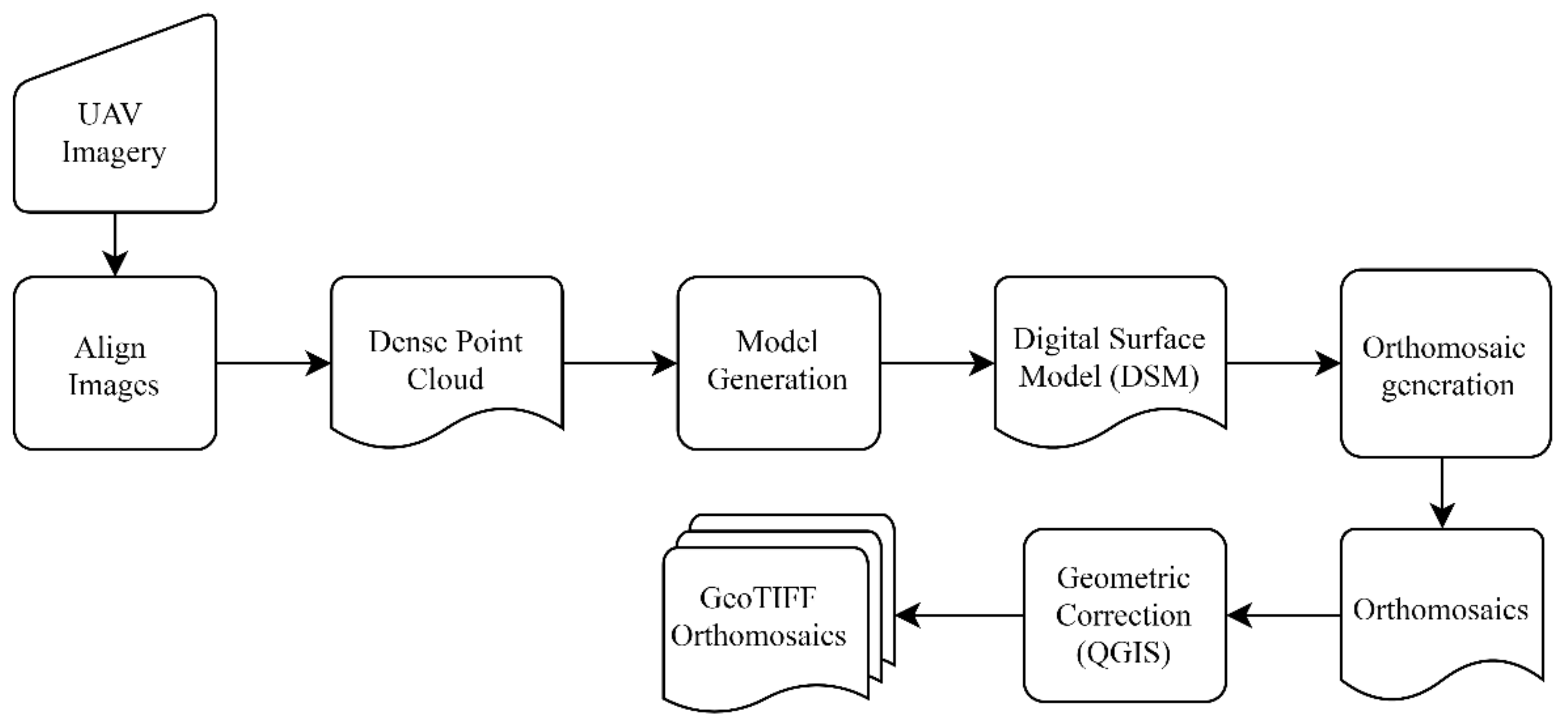
2.3. UAV Imagery Pre-Processing

All images were recorded in RAW format and after processing converted to the Tagged Image File Format (TIFF). The images were processed in the Agisoft™ MetaShape software, version 1.5.3 (Agisoft LLC, St. Petersburg, Russia). The RedEdge MX images were radiometrically calibrated using the correction factors of the Micasense’s calibration target, and the RGB camera images were calibrated using the vicarious method [31,32,33]. For that, the pixels of the four PVC targets were manually clipped. Then, linear regression models for each three-band were adjusted using the average pixel digital number (DN) and reflectance values of the targets obtained with the spectroradiometer. The DN values in the whole images were converted to reflectance based on the regression equations.
Subsequently, all images were processed to create the orthomosaics. Firstly, all five bands from the RedEdge MX needed to be aligned since the sensor acquires one image per channel. Thus, the five bands were aligned and grouped in a single file for each multispectral image. Then, the orthomosaics of both cameras were created performing the following steps: (1) image alignment using the UAV’s GPS unit; (2) construction of a three-dimensional point cloud using the Structure from Motion (SfM) technique [34,35]; (3 and 4) creation of the dense point cloud, which served as the basis for creating the Digital Surface Model (DSM); (5) the DSM was used to project every image pixel to generate the orthomosaics [36,37]; and finally, (6), using the QGIS, version 3.2 [38], all orthomosaics were georeferenced using the GCP coordinates (Figure 3).

2.4. Laboratory Experiment for Coffee Fruit Ripeness Spectra Characterization

Spectral reflectance patterns of the coffee fruits are useful to understand the main differences and challenges of monitoring their ripeness at the field level from that observed in the UAV images. Based on that, a laboratory reflectance spectroscopy experiment was performed to characterize the spectral pattern of the fruit ripeness. Five samples of coffee fruits (500 fruits per sample) with different percentages of unripe and ripe fruits were conditioned in a flat surface, 8 cm from the spectroradiometer and 80 cm from two halogen lamps (300 W) (Figure 4). Five measurements per sample were performed using the spectroradiometer.

2.5. Extraction of the Vegetation Indices and Field Assessments of the Coffee Ripeness

From the GeoTIFF orthomosaics, the following VIs were obtained for the study area: the Coffee Ripeness Index (CRI); the Green-red Ratio Ripeness Index (GRRI); the Modified Chlorophyll Absorption in Reflectance Index 1 (MCARI1); the Normalized Difference Vegetation Index (NDVI); the Normalized Difference RedEdge Index (NDRE); and the Green Normalized Difference Vegetation Index (GNDVI) (Table 3). The GRRI was selected because it was previously created to assess the coffee ripeness using UAV imagery, whereas the MCARI1, NDVI, NDRE, and GNDVI were selected due to their good relationship with vegetation pigments, as well as to their extensive use in crop monitoring studies. Those five VIs were chosen for comparison purposes with the CRI.
The VIs were obtained at the sampling point level, which was defined considering three plants in the same cultivation row. After calculating the IVs, polygonal masks were manually created for each sampling point using the QGIS software. Then, the average values of the polygon pixels were extracted using the zonal statistics tool.
For the validation of the VIs, manual measurements of the coffee ripeness were carried out on the same dates of image acquisition (Table 2). An irregular grid with 20 samples per hectare was set up on each measurement day for the fields A, C, D, and E. For field B, only 10 samples per hectare were considered due to its lower fruit load. Furthermore, on each plant, four plagiotropic branches were randomly chosen in the plant’s middle third, considering one branch per quadrant. After that, the unripe fruits, and the total of fruits on the branches of each plant were counted and the average value was used to represent each sampling point. Finally, using the percentage of unripe fruits, the sampling points were classified into two ripeness class: not ready for harvest with more than 30% of unripe fruits; and ready for harvest with the percentage of unripe fruits with less than 30%. This proportion has been used by the farmers in the region to begin the harvest.

2.6. Statistical Analysis

Initially, an analysis of variance (ANOVA) was carried out between the ripeness classes to evaluate the potential of the six VI to discriminate plants that were ready to harvest from not-ready in the field. First, this analysis was performed for each coffee field, and then, all data were grouped into a single dataset to evaluate the influence of the different cultivars, crop canopy and yield on the VIs performance.
Next, linear regression (Y = β0 + β1X) was used to model the relationship of the VIs and the field coffee ripeness. In addition, the significance of the regression coefficients was evaluated using the t-test at 1% probability (p < 0.01). Finally, to infer about which VI presented better adjustment to the coffee ripeness, the following statistical metrics were calculated: Coefficient of determination (R2), and Root mean square error (RMSE). All statistical analyses were performed using the R software, version 3.6.1 [42].

3. Results

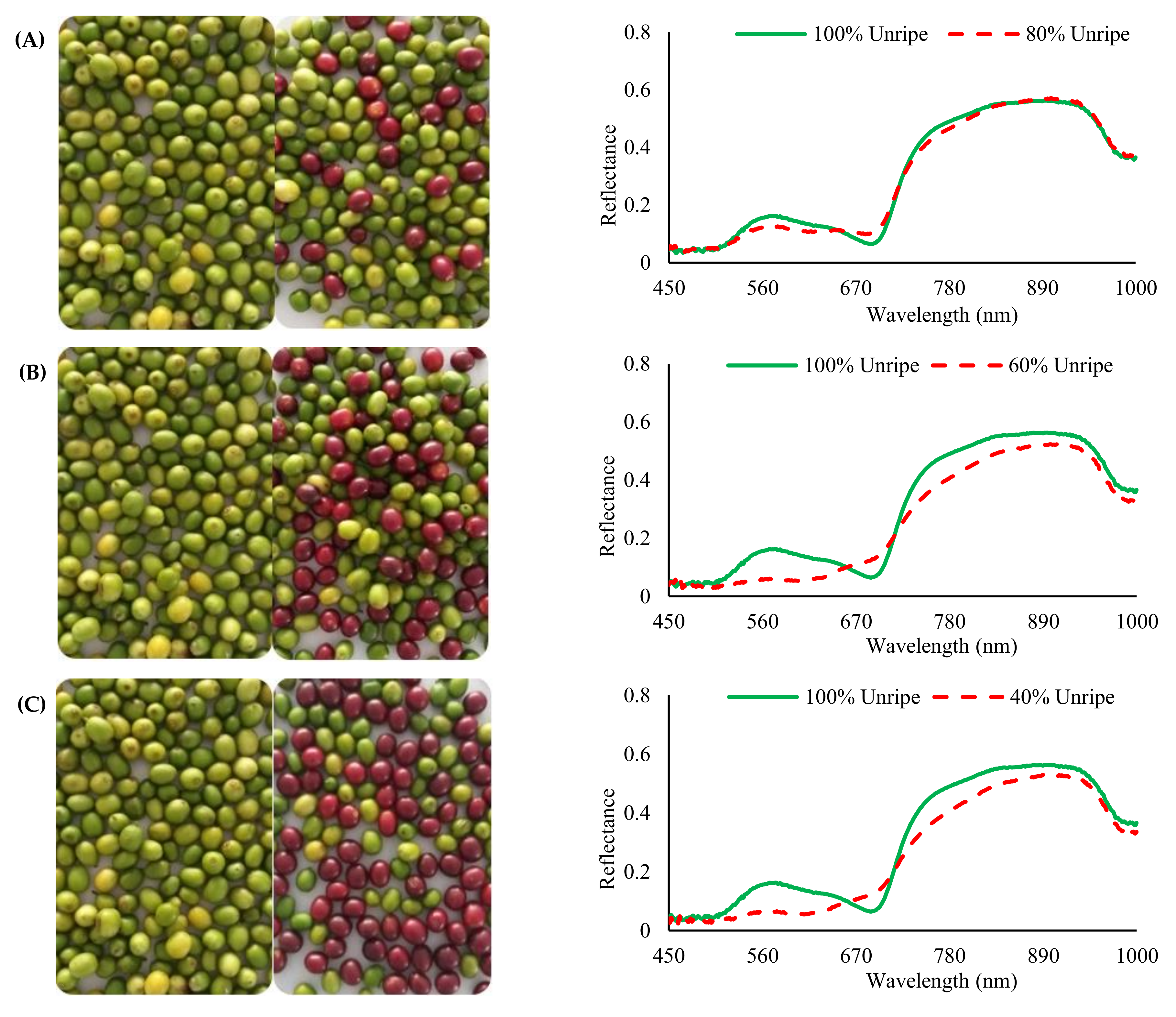
3.1. Spectral Characterization of Coffee Fruits Ripeness

Measurements done in laboratory showed that the coffee fruits spectra are highly variable according to the fruit ripeness degree (Figure 5). As expected, unripe fruits presented a reflectance peak in the green band (560 nm ± 20 nm), whereas in the red band (650 ± 30 nm) it showed an absorption peak, possibly related to the higher amount of chlorophyll in this region [7]. Then, the reflectance increased until the 900 nm in the NIR region. Conversely, after reducing the percentage of unripe fruits (Figure 5A–E), the samples tended to present a flat spectral behavior up to the red band, where it presented a reflectance peak, which is related to the reduction of chlorophyll pigments and accumulation of anthocyanins [7]. After that, there was an increase in reflectance as observed in the sample with 0% of unripe fruits (Figure 5E).
In addition, the results also showed that the R, G and NIR bands presented better discrimination of unripe and ripe coffee fruits, while in the RedEdge band (717 nm ± 10 nm) the spectra from both classes tended to overlap around 720 nm. These bands are important to discriminate plants with unripe from those with ripe fruits, in which the differences can be detected using the VIs. Besides that, if we consider the application of the method in field conditions, the R band should be highlighted over the G and NIR bands since the coffee crop reflects a higher proportion of the G and NIR radiation. This characteristic can make it difficult to differentiate coffee fruits from leaves at 60 m height (UAV imagery). Thus, the R band is better since a subtle increase in its reflectance (i.e., increase of fruit ripeness) can be easier to detect than when using the G and NIR bands, in which a reduction of their reflectance cannot discriminate the coffee ripeness due to the spectral confusion among leaves and unripe fruits.

3.2. Potential of VIs for Discrimination of Coffee Ripeness Classes

The characterization of the arabica coffee fields used in this study is shown in Table 4. The study area is represented by different coffee cultivars and each coffee field presented different canopy volumes, density of plants, and crop yield. Additionally, the terrain of the region is mountainous, and the slope varied throughout the coffee fields. Regarding the crop yield, the field B that had the highest cultivation area, showed, on the other hand, the lowest yield among all fields. This lower yield is a result of the biennial yield effect, a peculiar characteristic of this crop which exhibits high and low yield values in alternated years.
Results of the ANOVA showed that only the CRI (both cameras), GRRI (RGB camera), and the MCARI1 were able to discriminate the coffee plants ready for harvest from not-ready for harvest (i.e., plants with unripe fruits from plants with ripe fruits), for all coffee fields (Table 5). Conversely, the GRRI when obtained from the RedEdge MX showed significant differences only in the fields A, B, and E. This result can be associated with different factors, such as the size of the dataset among cameras, temporal variability of the VI, and especially the specific characteristics of each coffee field.
Regarding the other VIs, the NDRE presented the best results for discriminating the coffee ripeness, in which only the field C presented no significant differences between ripeness classes. Conversely, the NDVI showed significant differences only for field D and E, whereas the GNDVI was only significant in field 2. Moreover, those coffee fields where the ripeness classes were not discriminated by the VIs, presented either higher canopy volumes or higher plant density (Table 4).
A second ANOVA was performed considering the data from all coffee fields as a single dataset. This analysis aimed to evaluate the influence of the different crop characteristics on the VIs performance. Results showed that only the CRI, GRRI, MCARI1, and NDRE presented significant (p < 0.001) differences between the ripeness classes. Furthermore, the information presented in Figure 6, especially the two circles, reinforces the information that pixels of the VIs on the crop canopy could effectively discriminate plants with unripe fruits from those with ripe fruits. In addition, the boxplots make clear that the CRI and MCARI1 presented the higher threshold among the ripeness classes, whereas, for the GRRI and NDRE there was some overlapping between classes.

3.3. Relationship between VIs and Coffee Ripeness

Results of the statistical metrics obtained with the five VIs for estimation of the coffee ripeness are presented in Figure 7. From a general point of view, it can be observed that the linear models used for estimation of the coffee ripeness showed satisfactory adjustments (i.e., R2 and RMSE) considering the characteristics of the fields. Overall, the highest R2 and lowest RMSE values were obtained in field C (R2: 0.70; RMSE: 12.42%) and A (R2: 0.68; RMSE: 12.86%) by the CRI using the RedEdge MX, followed by MCARI1 (Field A and C, R2: 0.66 and 0.67; RMSE: 13.77 and 13.28%) and the CRI from the RGB camera (Field A and C, R2: 0.62 and 0.62; RMSE: 15.43 and 14.35%).
Regarding the other VIs, they presented on the best-case scenarios R2 values of 0.51 (Field A), 0.48 (Field D), 0.47 (Field B), 0.22 (Field E), and 0.26 (Field B) and RMSE values of 16.50, 14.92, 13.42, 14.74, and 15.88%, respectively for the GRRI (RedEdge MX and RGB camera), NDRE, NDVI, and the GNDVI. Besides that, when considering all coffee fields as a single dataset, the linear models from all VIs presented lower performances. Moreover, it is worth mentioning that the differences in the statistical metrics between fields are related to the specific characteristics and dataset size of each coffee field.
Due to the large amount of data, only the linear models that ranked best on the R2 and RMSE metrics are presented in Figure 8. Overall, the CRI (RedEdge MX) performed best in all fields, except to field E, where the MCARI1 was better fit to the data. In addition, the version derived from the RedEdge MX presented higher performance than its version from the RGB camera in all coffee fields. Despite that, these VIs showed good results considering the variability between fields and the non-uniform fruit ripeness presented by the crop, which makes it harder to develop a universal model for coffee ripeness estimation.

4. Discussion

Coffee fruit ripeness monitoring is a crucial indicator for defining the optimal harvest time, especially because unlike unripe and overripe fruits, the ripe fruits (cherries) tend to produce beverages with higher quality [5]. Remote sensing is an effective approach that has been widely used to investigate crop parameters, in which some studies resulted in the development of several vegetation indices [11,26,43,44]. In this study, a simple and effective VI based on a single spectral band was developed using UAV imagery for coffee fruit ripeness monitoring.
The CRI outperformed traditional VIs such as the MCARI1, NDVI, NDRE, GNDVI, and also the GRRI, which was previously developed for coffee ripeness monitoring [23]. However, the field characteristics such as plant density, canopy volume and especially, the crop yield directly influenced the VIs performance. The spectral response of a crop canopy tend to be similar to that of a single leaf, but changeable by many factors such as plant tissue optical properties, canopy structure, plant physiology, and climatic conditions [45,46,47]. For the coffee crop, there is an additional factor, the unequal fruit ripening, which is practically inevitable under natural conditions because coffee blossoming in nonequatorial regions as in the southcentral Brazil occurs at different times in the same season (e.g., from August to November) in most of the production areas [28]. These factors made it more challenging to differentiate coffee fruits (unripe and ripe) from leaves when the VIs were used.
As stated before, at the laboratory level, the spectra of unripe and ripe fruits can be easily differentiated as the percentage of unripe fruits reduces (Figure 5). However, it can be very difficult to differentiate them using aerial imagery, especially under highly dense crop canopies that can induce spectral confusion. For the initial analysis, the CRI, GRRI (RGB camera), and MCARI1 were the only VIs capable of discriminating the ripeness classes in all coffee fields. The GRRI (RedEdge MX) and NDRE presented satisfactory performances, yet they were still influenced by field characteristics. On the other hand, the worst performance was presented by the NDVI and GNDVI that saturated, especially in the fields with higher plant density and canopy volume (Table 4). This problem has been addressed in other studies, whose authors reported the influence of several factors related to crop species, leaf area, crop biomass, it foliage, and others [13,48,49,50].
When the five fields dataset was grouped, only the CRI, GRRI, MCARI1, and NDRE showed significant differences between the ripeness classes. This result is related to the temporal fruit color change, which is caused by the disappearance of chlorophyll pigments and the accumulation of anthocyanins [7] that altered the crop canopy spectral response (Figure 6). Besides that, from the fruit filling to the ripeness stage, coffee plants present a high nutritional demand, especially for NPK, which leads to an increase in nutrient translocation from the leaves to the fruits [51]. This can result in nutrient deficiency and also in changes of leaf reflectance in the visible (400–700 nm) and NIR (700–1100 nm) wavelengths [52], which can be better-detected with VIs of higher sensitivity to chlorophyll pigments [53,54,55]. Together, these factors led these VIs, and especially the CRI due to its higher sensitivity of changes in the red wavelength, to present better capability of discriminating plants with unripe fruits from those with ripe fruits.
For the regression analysis, the CRI outperformed the other VIs on most coffee fields, except to field 5 where the MCARI1 showed better performance (Figure 7 and Figure 8). Compared to this study, [23] developed and tested the GRRI for ripeness monitoring in nine coffee fields and obtained a R2 of 0.43. On the other hand, [9], using the same index reported a much better correlation (R2: 0.81) for seven coffee fields. However, these authors presented the results at the field level, which does not entirely represent the spatial variability of the fruit ripeness. Moreover, all coffee fields presented high fruit display on the canopy exterior. Differently, in this study, the sampling points were defined at every three plants, which better represented the spatial variability of fruit ripeness. In addition, not all five coffee fields presented high yield, which as discussed before, played a major role in the VIs performance. In this sense, our results were more satisfactory than those presented above, especially due to the higher sensitivity shown by the CRI in detecting the fruit ripeness changes.
Regarding the results obtained with the CRI and GRRI from both cameras, the differences in the ANOVA and linear regression analysis are related to the radiometric calibration method and mainly to the dataset size of both cameras. The RedEdge MX besides presenting an individual CMOS for each band, it presents a more complex calibration system composed by its downwelling light sensor and the factory-calibrated reference target (For more details look at [56,57]). On the other hand, in the RGB camera due to the absence of a calibration system, we used low-cost targets and the vicarious calibration, a simple and effective method [58]; but not as robust as the one presented by the RedEdge MX.
Apart from that, the dataset size was the main factor influencing the VIs results. The RGB camera was used in four weeks, whereas the RedEdge MX was used only in the third and fourth weeks due to availability (Table 2). During the two first weeks, there was a higher percentage of unripe fruits than in the last two weeks. This increased the temporal variability of the fruit ripeness and resulted in lower performance by the CRI from the RGB camera. Conversely, the version derived from the RedEdge MX presented a better result due to the higher percentage of ripe fruits in the last weeks, which could be detected from the crop canopy. Differently, the GRRI (RGB camera) was positively influenced by the higher number of samples, unlike its other version (Table 5 and Figure 7).
In addition, the magnitude of the CRI and GRRI values from the RGB camera was different than the ones derived from the RedEdge MX. This result is possibly associated with the sensitivity of the CMOs that can be variable among different wavelengths [59]. For the RGB camera, the same settings of ISO and shutter aperture are used since its single sensor is used to register the information from RGB bands. Conversely, the RedEdge MX does not present this limitation since there is one CMOs for each band, whose settings are individually adjusted according to the band’s specifications. Regardless, both VIs obtained with the RGB camera presented satisfactory results, especially the CRI. In this sense, the RGB camera use can be a feasible alternative to monitor the coffee ripeness, especially in small farms due to its lower cost compared to the RedEdge MX.
Overall, our findings corroborate those stated by other authors [9,23], in which the use of RS in the coffee crop for fruit ripeness monitoring is still challenging due to the plant architecture and the high canopy volume presented by most cultivars. In addition, another characteristic that plays a major role in the performance of RS-based methodologies in the coffee crop is the crop yield. Due to the biennial effect, the crop yield alternates between low and high yields every year [13]. This characteristic has a direct influence on the number of fruits displayed on the crop canopy, which end up affecting the performance of the VIs. Despite that, the study demonstrated that the time-consuming manual fruit counts made on a few plants can be replaced by remote sensing approaches. Furthermore, these results fill a gap in the literature of remote sensing studies related to the coffee fruit ripeness monitoring, which is a key factor for defining the beverage quality. Lastly, a recommendation for future studies would be the use of the CRI and other variables (e.g., solar radiation, degrees Brix, canopy temperature, etc.) for prediction of fruit ripeness and beverage quality using machine learning algorithms.

5. Conclusions

In this study, a simple and effective vegetation index (VI) was proposed for coffee ripeness estimation using aerial imagery. The Coffee ripeness index (CRI) was developed, combining reflectance from the red band and from a ground-based red target. The effectiveness of the CRI was compared in different analysis with traditional VIs such as the MCARI1, NDVI, NDRE, GNDVI, and the GRRI in five coffee fields under distinct cultivation characteristics.
The CRI showed a higher sensitivity to discriminate coffee plants ready for harvest from not-ready for harvest in all coffee fields. However, the field characteristics such as plant density, canopy volume and especially, the crop yield played a key role in the VIs performance. Therefore, the methodology based on VIs, especially the CRI, can yield better results on coffee fields with higher fruit display on the canopy exterior.
Regarding the two cameras evaluated, both of them presented satisfactory results. However, the RGB camera use can be a feasible alternative to monitor the coffee ripeness, especially in small farms due to its lower cost compared to the RedEdge MX. Finally, the study demonstrated that the time-consuming fieldwork can be replaced by the methodology based on VIs.

Author Contributions

Conceptualization, R.N.M. and F.d.A.d.C.P.; Formal analysis, R.N.M.; Funding acquisition, F.d.A.d.C.P.; Investigation, R.N.M.; Methodology, R.N.M.; Project administration, F.d.A.d.C.P.; Resources, D.M.d.Q.; Supervision, F.d.A.d.C.P., D.M.d.Q. and D.S.M.V.; Validation, J.T.F.R.; Visualization, J.T.F.R.; Writing—original draft, R.N.M.; Writing—review & editing, R.N.M., F.d.A.d.C.P., D.M.d.Q., D.S.M.V. and J.T.F.R. All authors have read and agreed to the published version of the manuscript.

Funding

This study was partially financed by the Coordenação de Aperfeiçoamento de Pessoal de Nível Superior (CAPES, Coordination for the Improvement of Higher Education Personnel)–Finance Code 001, and by the Conselho Nacional de Desenvolvimento Científico e Tecnológico (CNPq, The Brazilian National Council for Scientific and Technological Development)-Grant number 144740/2019-2.

Institutional Review Board Statement

Not applicable.

Informed Consent Statement

Not applicable.

Data Availability Statement

The data presented in this study are available on request from the author (R.N.M.).

Acknowledgments

We thank the Department of Agricultural Engineering (DEA) of the Universidade Federal de Viçosa for supporting the researchers.

Conflicts of Interest

The authors declare no conflict of interest.

References

  1. International Coffee Organization (ICO). Historical Data on the Global Coffee Trade; International Coffee Organization (ICO): London, UK, 2020. [Google Scholar]
  2. USDA. Coffee: World Markets and Trade (Issue June). 2020. Available online: http://apps.fas.usda.gov/psdonline/circulars/coffee.pdf (accessed on 10 September 2020).
  3. De Assis Silva, S.; de Souza LIMA, J.S.; Alves, A.I. Spatial study of grain yield and percentage of bark of two varieties of Coffea arabica L. to the production of quality coffee. Biosci. J. 2010, 26, 558–565. [Google Scholar]
  4. Martinez, H.E.P.; Poltronieri, Y.; Farah, A.; Perrone, D. Zinc supplementation, production and quality of coffee beans. Rev. Ceres 2013, 60, 293–299. [Google Scholar] [CrossRef] [Green Version]
  5. Silva, S.D.A.; De Queiroz, D.M.; Pinto, F.D.A.C.; Santos, N.T. Coffee quality and its relationship with Brix degree and colorimetric information of coffee cherries. Precis. Agric. 2014, 15, 543–554. [Google Scholar] [CrossRef]
  6. Fagan, E.B.; de Souza, C.H.E.; Pereira, N.M.B.; Machado, V.J. Efeito do tempo de formação do grão de café (Coffea sp.) na qualidade da bebida. Biosci. J. 2011, 27. [Google Scholar]
  7. De Castro, R.D.; Marraccini, P. Cytology, biochemistry and molecular changes during coffee fruit development. Braz. J. Plant Physiol. 2006, 18, 175–199. [Google Scholar] [CrossRef] [Green Version]
  8. Aparecido, L.; Rolim, G.D.S.; Moraes, T.; Valeriano, T.T.B.; Lense, G.H.E. Maturation periods for Coffea arabica cultivars and their implications for yield and quality in Brazil. J. Sci. Food Agric. 2018, 98, 3880–3891. [Google Scholar] [CrossRef]
  9. Herwitz, S.; Johnson, L.; Dunagan, S.; Higgins, R.; Sullivan, D.; Zheng, J.; Lobitz, B.; Leung, J.; Gallmeyer, B.; Aoyagi, M.; et al. Imaging from an unmanned aerial vehicle: Agricultural surveillance and decision support. Comput. Electron. Agric. 2004, 44, 49–61. [Google Scholar] [CrossRef]
  10. Furfaro, R.; Ganapol, B.; Johnson, L.F.; Herwitz, S.R. Neural Network Algorithm for Coffee Ripeness Evaluation Using Airborne Images. Appl. Eng. Agric. 2007, 23, 379–387. [Google Scholar] [CrossRef]
  11. Ren, Y.; Meng, Y.; Huang, W.; Ye, H.; Han, Y.; Kong, W.; Zhou, X.; Cui, B.; Xing, N.; Guo, A.; et al. Novel Vegetation Indices for Cotton Boll Opening Status Estimation Using Sentinel-2 Data. Remote. Sens. 2020, 12, 1712. [Google Scholar] [CrossRef]
  12. Coltri, P.P.; Zullo, J.; do Valle Goncalves, R.R.; Romani, L.A.S.; Pinto, H.S. Coffee Crop’s Biomass and Carbon Stock Estimation With Usage of High-Resolution Satellites Images. IEEE J. Sel. Top. Appl. Earth Obs. Remote Sens. 2013, 6, 1786–1795. [Google Scholar] [CrossRef]
  13. Bernardes, T.; Moreira, M.A.; Adami, M.; Giarolla, A.; Rudorff, B.F.T. Monitoring Biennial Bearing Effect on Coffee Yield Using MODIS Remote Sensing Imagery. Remote Sens. 2012, 4, 2492–2509. [Google Scholar] [CrossRef] [Green Version]
  14. Nogueira, S.M.C.; Moreira, M.A.; Volpato, M.M.L. Relationship between coffee crop productivity and vegetation indexes derived from oli/landsat-8 sensor data with and without topographic correction. Eng. Agric. 2018, 38, 387–394. [Google Scholar] [CrossRef]
  15. Tsai, D.-M.; Chen, W.-L. Coffee plantation area recognition in satellite images using Fourier transform. Comput. Electron. Agric. 2017, 135, 115–127. [Google Scholar] [CrossRef]
  16. Ramirez, G.M.; Zullo, J., Jr. Estimation of biophysical parameters of coffee fields based on high-resolution satellite images. Eng. Agric. 2010, 30, 468–479. [Google Scholar]
  17. Miranda, J.D.R.; Alves, M.D.C.; Pozza, E.A.; Neto, H.S. Detection of coffee berry necrosis by digital image processing of landsat 8 oli satellite imagery. Int. J. Appl. Earth Obs. Geoinf. 2020, 85, 101983. [Google Scholar] [CrossRef]
  18. Carrijo, G.L.A.; Oliveira, D.E.; De Assis, G.A.; Carneiro, M.G.; Guizilini, V.C.; Souza, J.R. Automatic detection of fruits in coffee crops from aerial images. In Proceedings of the 2017 Latin American Robotics Symposium (LARS) and 2017 Brazilian Symposium on Robotics (SBR), Curitiba, Brazil, 8–11 November 2017; pp. 1–6. [Google Scholar]
  19. Da Cunha, J.P.A.R.; Neto, M.A.S.; Hurtado, S.M.C. Estimating vegetation volume of coffee crops using images from unmanned aerial vehicles. Eng. Agric. 2019, 39, 41–47. [Google Scholar] [CrossRef]
  20. Dos Santos, L.M.; Ferraz, G.A.E.S.; Barbosa, B.D.; Diotto, A.V.; Maciel, D.T.; Xavier, L.A.G. Biophysical parameters of coffee crop estimated by UAV RGB images. Precis. Agric. 2020, 21, 1227–1241. [Google Scholar] [CrossRef]
  21. Santos, L.M.; Ferraz, G.A.S.; Diotto, A.V.; Barbosa, B.D.S.; Maciel, D.T.; Andrade, M.T.; Ferraz, P.F.P.; Rossi, G. Coffee crop coefficient prediction as a function of biophysical variables identified from RGB UAS images. Agron. Res. 2020, 18, 1463–1471. [Google Scholar] [CrossRef]
  22. Parreiras, T.C.; Lense, G.H.E.; Moreira, R.S.; Santana, D.B.; Mincato, R.L. Using unmanned aerial vehicle and machine learning algorithm to monitor leaf nitrogen in coffee. Coffee Sci. 2020, 15, 1–9. [Google Scholar] [CrossRef]
  23. Johnson, L.F.; Herwitz, S.; Lobitz, B.M.; Dunagan, S.E. Feasibility of monitoring coffee field ripeness with airborne multispectral imagery. Appl. Eng. Agric. 2004, 20, 845–849. [Google Scholar] [CrossRef]
  24. Rouse, J.W.; Haas, R.H.; Schell, J.A.; Deeering, D. Monitoring vegetation systems in the Great Plains with ERTS (Earth Resources Technology Satellite). In Proceedings of the Third Earth Resources Technology Satellite-1 Symposium, NASA, Goddard Space Flight Center, Washington, DC, USA, 10–14 December 1973. [Google Scholar]
  25. Huete, A. A soil-adjusted vegetation index (SAVI). Remote. Sens. Environ. 1988, 25, 295–309. [Google Scholar] [CrossRef]
  26. Baloloy, A.B.; Blanco, A.C.; Ana, R.R.C.S.; Nadaoka, K. Development and application of a new mangrove vegetation index (MVI) for rapid and accurate mangrove mapping. ISPRS J. Photogramm. Remote Sens. 2020, 166, 95–117. [Google Scholar] [CrossRef]
  27. Moreira, M.A.; Adami, M.; Theodor, F. Análise espectral e temporal da cultura do café em imagens Landsat Spectral and temporal behavior analysis of coffee crop in Landsat images. Pesqui. Agropecuária Bras. 2004, 39, 223–231. [Google Scholar] [CrossRef]
  28. Da Matta, F.M.; Ronchi, C.P.; Maestri, M.; Barros, R.S. Ecophysiology of coffee growth and production. Braz. J. Plant Physiol. 2007, 19, 485–510. [Google Scholar] [CrossRef] [Green Version]
  29. Alvares, C.A.; Stape, J.L.; Sentelhas, P.C.; Gonçalves, J.L.D.M.; Sparovek, G. Köppen’s climate classification map for Brazil. Meteorol. Z. 2013, 22, 711–728. [Google Scholar] [CrossRef]
  30. Javan, F.D.; Samadzadegan, F.; Pourazar, S.H.S.; Fazeli, H. UAV-based multispectral imagery for fast Citrus Greening detection. J. Plant Dis. Prot. 2019, 126, 307–318. [Google Scholar] [CrossRef]
  31. Del Pozo, S.; Rodríguez-Gonzálvez, P.; Hernández-López, D.; Felipe-García, B. Vicarious Radiometric Calibration of a Multispectral Camera on Board an Unmanned Aerial System. Remote Sens. 2014, 6, 1918–1937. [Google Scholar] [CrossRef] [Green Version]
  32. Wang, C.; Myint, S.W. A Simplified Empirical Line Method of Radiometric Calibration for Small Unmanned Aircraft Systems-Based Remote Sensing. IEEE J. Sel. Top. Appl. Earth Obs. Remote Sens. 2015, 8, 1876–1885. [Google Scholar] [CrossRef]
  33. Rosas, J.T.F.; Pinto, F.D.A.D.C.; De Queiroz, D.M.; Villar, F.M.D.M.; Martins, R.N.; Silva, S.D.A. Low-cost system for radiometric calibration of UAV-based multispectral imagery. J. Spat. Sci. 2020, 1–15. [Google Scholar] [CrossRef]
  34. Brenner, C.; Zeeman, M.; Bernhardt, M.; Schulz, K. Estimation of evapotranspiration of temperate grassland based on high-resolution thermal and visible range imagery from unmanned aerial systems. Int. J. Remote Sens. 2018, 39, 5141–5174. [Google Scholar] [CrossRef] [Green Version]
  35. Zarco-Tejada, P.J.; Diazvarela, R.; Angileri, V.; Loudjania, P. Tree height quantification using very high-resolution imagery acquired from an unmanned aerial vehicle (UAV) and automatic 3D photo-reconstruction methods. Eur. J. Agron. 2014, 55, 89–99. [Google Scholar] [CrossRef]
  36. Ashapure, A.; Jung, J.; Yeom, J.; Chang, A.; Maeda, M.; Maeda, A.; Landivar, J. A novel framework to detect conventional tillage and no-tillage cropping system effect on cotton growth and development using multi-temporal UAS data. ISPRS J. Photogramm. Remote Sens. 2019, 152, 49–64. [Google Scholar] [CrossRef]
  37. Wijesingha, J.; Astor, T.; Schulze-Brüninghoff, D.; Wengert, M.; Wachendorf, M. Predicting Forage Quality of Grasslands Using UAV-Borne Imaging Spectroscopy. Remote Sens. 2020, 12, 126. [Google Scholar] [CrossRef] [Green Version]
  38. QGIS Development Team. QGIS Geographic Information System. Open Source Geospat. Found. Proj. 2016. Available online: http://qgis.osgeo.org (accessed on 10 June 2020).
  39. Haboudane, D.; Miller, J.R.; Pattey, E.; Zarco-Tejada, P.J.; Strachan, I.B. Hyperspectral vegetation indices and novel algorithms for predicting green LAI of crop canopies: Modeling and validation in the context of precision agriculture. Remote Sens. Environ. 2004, 90, 337–352. [Google Scholar] [CrossRef]
  40. Fitzgerald, G.; Rodriguez, D.; Christensen, L.K.; Belford, R.; Sadras, V.O.; Clarke, T.R. Spectral and thermal sensing for nitrogen and water status in rainfed and irrigated wheat environments. Precis. Agric. 2006, 7, 233–248. [Google Scholar] [CrossRef]
  41. Gitelson, A.A.; Kaufman, Y.J.; Merzlyak, M.N. Use of a green channel in remote sensing of global vegetation from EOS-MODIS. Remot. Sens. Environ. 1996, 58, 289–298. [Google Scholar] [CrossRef]
  42. Team, R.C. R: A Language and Environment for Statistical Computing; R Foundation for Statistical Computing: Vienna, Austria, 2019. [Google Scholar]
  43. Maimaitijiang, M.; Sidike, P.; Sidike, P.; Maimaitiyiming, M.; Hartling, S.; Peterson, K.T.; Maw, M.J.; Shakoor, N.; Mockler, T.; Fritschi, F.B. Vegetation Index Weighted Canopy Volume Model (CVMVI) for soybean biomass estimation from Unmanned Aerial System-based RGB imagery. ISPRS J. Photogramm. Remote. Sens. 2019, 151, 27–41. [Google Scholar] [CrossRef]
  44. He, J.; Zhang, N.; Su, X.; Lu, J.; Yao, X.; Cheng, T.; Zhu, Y.; Cao, W.; Tian, Y. Estimating Leaf Area Index with a New Vegetation Index Considering the Influence of Rice Panicles. Remote Sens. 2019, 11, 1809. [Google Scholar] [CrossRef] [Green Version]
  45. Hede, A.N.H.; Kashiwaya, K.; Koike, K.; Sakurai, S. A new vegetation index for detecting vegetation anomalies due to mineral deposits with application to a tropical forest area. Remote Sens. Environ. 2015, 171, 83–97. [Google Scholar] [CrossRef] [Green Version]
  46. Koide, K.; Koike, K. Applying vegetation indices to detect high water table zones in humid warm-temperate regions using satellite remote sensing. Int. J. Appl. Earth Obs. Geoinf. 2012, 19, 88–103. [Google Scholar] [CrossRef]
  47. Zarco-Tejada, P.J.; Miller, J.R.; Noland, T.L.; Mohammed, G.H.; Sampson, P.H. Scaling-up and model inversion methods with narrowband optical indices for chlorophyll content estimation in closed forest canopies with hyperspectral data. IEEE Trans. Geosci. Remote Sens. 2001, 39, 1491–1507. [Google Scholar] [CrossRef] [Green Version]
  48. Hunt, E.R.; Hively, W.D.; Daughtry, C.S.T.; Mccarty, G.W.; Fujikawa, S.J.; Ng, T.L.; Tranchitella, M.; Linden, D.S.; Yoel, D.W. Remote Sensing of Crop Leaf Area Index Using Unmanned Airborne Vehicles. In Proceedings of the Pecora 17 Conference, American Society for Photogrammetry and Remote Sensing, Denver, Colorado, 18–20 November 2008. [Google Scholar]
  49. Carneiro, F.M.; Furlani, C.E.A.; Zerbato, C.; De Menezes, P.C.; Gírio, L.A.D.S.; De Oliveira, M.F. Comparison between vegetation indices for detecting spatial and temporal variabilities in soybean crop using canopy sensors. Precis. Agric. 2019, 21, 979–1007. [Google Scholar] [CrossRef]
  50. Kross, A.; McNairn, H.; Lapen, D.; Sunohara, M.; Champagne, C. Assessment of RapidEye vegetation indices for estimation of leaf area index and biomass in corn and soybean crops. Int. J. Appl. Earth Obs. Geoinf. 2015, 34, 235–248. [Google Scholar] [CrossRef] [Green Version]
  51. Laviola, B.G.; Martinez, H.E.P.; De Souza, R.B.; Salomão, L.C.C.; Cruz, C.D. Macronutrient Accumulation in Coffee Fruits at Brazilian Zona Da Mata Conditions. J. Plant Nutr. 2009, 32, 980–995. [Google Scholar] [CrossRef]
  52. Ayala-Silva, T.; Beyl, C.A. Changes in spectral reflectance of wheat leaves in response to specific macronutrient deficiency. Adv. Space Res. 2005, 35, 305–317. [Google Scholar] [CrossRef] [PubMed]
  53. Lin, S.; Li, J.; Liu, Q.; Li, L.; Zhao, J.; Yu, W. Evaluating the Effectiveness of Using Vegetation Indices Based on Red-Edge Reflectance from Sentinel-2 to Estimate Gross Primary Productivity. Remote Sens. 2019, 11, 1303. [Google Scholar] [CrossRef] [Green Version]
  54. Huang, S.; Miao, Y.; Zhao, G.; Yuan, F.; Ma, X.; Tan, C.; Yu, W.; Gnyp, M.L.; Lenz-Wiedemann, V.; Rascher, U.; et al. Satellite Remote Sensing-Based In-Season Diagnosis of Rice Nitrogen Status in Northeast China. Remote Sens. 2015, 7, 10646–10667. [Google Scholar] [CrossRef] [Green Version]
  55. Sonobe, R.; Wang, Q. Hyperspectral indices for quantifying leaf chlorophyll concentrations performed differently with different leaf types in deciduous forests. Ecol. Inform. 2017, 37, 1–9. [Google Scholar] [CrossRef]
  56. Mamaghani, B.; Connal, R.; Hartzell, R.; Kha, K.; Sasaki, G.; Marcellus, E.; Knappen, J.; Bauch, T.; Raqueno, N.; Salvaggio, C. An initial exploration of vicarious and in-scene calibration techniques for small unmanned aircraft systems. Auton. Air Ground Sens. Syst. Agric. Optim. Phenotyping III 2018, 10664, 1066406. [Google Scholar] [CrossRef]
  57. Mamaghani, B.; Salvaggio, C. Multispectral Sensor Calibration and Characterization for sUAS Remote Sensing. Sensors 2019, 19, 4453. [Google Scholar] [CrossRef] [Green Version]
  58. Iqbal, F.; Lucieer, A.; Barry, K. Simplified radiometric calibration for UAS-mounted multispectral sensor. Eur. J. Remote Sens. 2018, 51, 301–313. [Google Scholar] [CrossRef]
  59. Lule, T.; Benthien, S.; Keller, H.; Mutze, F.; Rieve, P.; Seibel, K.; Sommer, M.; Bohm, M. Sensitivity of CMOS based imagers and scaling perspectives. IEEE Trans. Electron Devices 2000, 47, 2110–2122. [Google Scholar] [CrossRef]
Figure 1. Location of the study area in Minas Gerais State, Southeastern Brazil.
Remotesensing 13 00263 g001
Figure 2. Spectral response curves (A) of the polyvinyl chloride-based (PVC) (B) calibration targets used during the flight campaigns.
Remotesensing 13 00263 g002
Figure 3. Workflow developed for processing the UAV images to obtain the georeferenced orthomosaics.
Remotesensing 13 00263 g003
Figure 4. Laboratory experiment set up used to characterize the spectra of the coffee fruit ripeness.
Remotesensing 13 00263 g004
Figure 5. Spectral reflectance patterns for different ripeness percentages of coffee fruits (A) 100% and 80% of unripe; (B) 100% and 60% of unripe; (C) 100% and 40% of unripe; (D) 100% and 20% of unripe; and (E) 100% of unripe and 100% of ripe fruits.
Remotesensing 13 00263 g005aRemotesensing 13 00263 g005b
Figure 6. Comparison of average values of the vegetation indices from plants with unripe (G) and ripe (R) coffee fruits in all fields. From right to the left: the rectangular boxes (AH) represent parts of the vegetation indices maps and the two central circles are examples of plant canopy under different ripeness classes. The boxplot presents the variation of the canopy spectral response from plants with unripe and ripe coffee fruits. p-values followed by *** are significant at 0.1% probability (p < 0.001); and ns, Not significant.
Remotesensing 13 00263 g006
Figure 7. Statistical metrics of the linear models for coffee ripeness estimation: (A) determination coefficient (R2); and (B) root mean square error (RMSE).
Remotesensing 13 00263 g007
Figure 8. Best ranked models adjusted to the coffee ripeness using the vegetation indices. (A) Field A; (B) Field B; (C) Field C; (D) Field D; (E) Field E; (F) All coffee fields; CRI, Coffee ripeness index using the RedEdge MX camera; MCARI1, Modified Chlorophyll Absorption in Reflectance Index 1; R2 values followed by *** are significant at 0.1 probability (p < 0.001).
Remotesensing 13 00263 g008
Table 1. Technical characteristics of the MicaSense RedEdge MX, and the Phantom 4 Pro Red, Green, Blue (RGB) camera.
CameraRedEdge MXPhantom 4 RGB
AcquisitionRGB–RE–NIRR–G–B
Sensor size (mm)4.8 × 3.64.7 × 6.3
Sensor size (px)1280 × 9605472 × 3648
Focal length (mm)5.48.8
Field of View (FOV)47.2°84°
Output formatRAW, TIF imageRAW, JPG image
R, Red; G, Green; B, Blue; RE, RedEdge; and NIR, Near-infrared.
Table 2. Unmanned Aerial Vehicles (UAV) data collection timeline and flight specifications.
DateAGL (m) 1Overlap (%) 2Spatial Resolution (cm)
29/04/201960−/75 3−/2.3
07/05/201960−/75−/2.3
13/05/20196080/755.0/2.3
27/05/20196080/755.0/2.3
1 Above ground level; 2 Lateral and longitudinal overlap; 3 The RedEdge MX was available only for the last two flights.
Table 3. References and equations of the spectral vegetation indices evaluated in this study.
Vegetation IndexEquationReference
CRI R / R target 100 Proposed VI
GRRI G / R [23]
MCARI1 1.2 2.5 NIR R   1.3 NIR G [39]
NDVI N R / N + R [24]
NDRE N RE / N + RE [40]
GNDVI N G / N + G [41]
N, Near-infrared; R, Red; G, Green; RE, RedEdge; and RTarget, Average reflectance value of the red target in the red band.
Table 4. Characteristics of the five arabica coffee fields used in this study.
FieldArea
(ha)
CultivarCanopy
Volume (m3)
Density
(Plants ha−1)
Average Slope
(%)
Yield
(kg ha−1)
A0.54Red Catuai2.91 ± 0.1940007.661220
B2.1Red Catuai1.87 ± 0.14400014.39480
C1.01MG H 419-10.62 ± 0.04800016.243750
D0.77Red Bourbon0.70 ± 0.0613,33323.762500
E0.65Icatu1.77 ± 0.10222220.792220
OBS: Coffee fruits from fields C and E present a yellow color when ripe.
Table 5. Comparison of average values of the vegetation indices from plants with unripe (G) and ripe (R) coffee fruits per field.
MicaSense RedEdge MX
FieldnClassCRIp-ValueGRRIp-ValueMCARI1p-ValueNDVIp-Value
A13G ± SD5.680 ± 0.8670.000 ***3.213 ± 0.5290.011 *0.450 ± 0.0690.000 ***0.823 ± 0.0140.772 ns
07R ± SD8.746 ± 0.774 2.621 ± 0.200 0.613 ± 0.038 0.821 ± 0.018
B27G ± SD6.509 ± 1.1930.000 ***3.246 ± 0.2550.000 ***0.480 ± 0.0440.000 ***0.821 ± 0.0170.067 ns
15R ± SD8.353 ± 1.519 2.924 ± 0.159 0.579 ± 0.057 0.810 ± 0.018
C25G ± SD6.740 ± 0.9220.000 ***3.034 ± 0.2950.257 ns0.493 ± 0.0750.000 ***0.812 ± 0.0220.891 ns
12R ± SD9.174 ± 0.834 2.912 ± 0.310 0.609 ± 0.029 0.811 ± 0.201
D18G ± SD6.354 ± 1.3430.000 ***3.178 ± 0.3110.121 ns0.474 ± 0.1390.000 ***0.847 ± 0.0110.017 *
12R ± SD9.727 ± 0.468 2.988 ± 0.202 0.725 ± 0.064 0.835 ± 0.010
E20G ± SD5.910 ± 0.9310.000 ***3.006 ± 0.2540.005 **0.396 ± 0.0690.000 ***0.803 ± 0.0100.016 *
08R ± SD9.094 ± 0.544 2.723 ± 0.111 0.521 ± 0.067 0.792 ± 0.009
Phantom 4 Pro RGB Camera MicaSense RedEdge MX
FieldnClassCRIp-ValueGRRIp-ValueNDREp-ValueGNDVIp-Value
A26G ± SD7.090 ± 1.5350.000 ***1.332 ± 0.2270.019 *0.556 ± 0.0200.000 ***0.847 ± 0.0050.069 ns
11R ± SD9.880 ± 1.292 1.132 ± 0.048 0.513 ± 0.021 0.841 ± 0.006
B61G ± SD7.118 ± 1.4500.001 **1.284 ± 0.1930.005 **0.549 ± 0.0230.002 **0.843 ± 0.0110.041 *
19R ± SD8.460 ± 1.006 1.140 ± 0.047 0.520 ± 0.030 0.835 ± 0.010
C48G ± SD6.075 ± 1.3920.000 ***1.255 ± 0.2210.014 *0.555 ± 0.0220.097 ns0.845 ± 0.0140.097 ns
16R ± SD8.190 ± 0.926 1.084 ± 0.046 0.541 ± 0.026 0.837 ± 0.008
D45G ± SD6.998 ± 1.6130.004 **1.202 ± 0.2150.000 ***0.547 ± 0.0100.000 ***0.848 ± 0.0070.053 ns
11R ± SD8.744 ± 0.632 0.915 ± 0.074 0.530 ± 0.006 0.839 ± 0.012
E44G ± SD6.831 ± 0.9580.000 ***1.184 ± 0.1340.001 **0.526 ± 0.0280.022 *0.832 ± 0.0100.165 ns
08R ± SD8.171 ± 0.257 1.007 ± 0.135 0.501 ± 0.015 0.826 ± 0.011
G, Average values of the vegetation indices from plants with unripe coffee fruits; R, Average values of the vegetation indices from plants with ripe coffee fruits; and SD, Standard deviation; ns, Not significant; p-values followed by ***, **, and * are significant at 0.1, 1, and 5% probability (p < 0.001; p < 0.01; p < 0.05).
Publisher’s Note: MDPI stays neutral with regard to jurisdictional claims in published maps and institutional affiliations.

