Next Article in Journal
A Novel Vegetation Index for Coffee Ripeness Monitoring Using Aerial Imagery
Next Article in Special Issue
Estimating Forest Structure from UAV-Mounted LiDAR Point Cloud Using Machine Learning
Previous Article in Journal
Predicting Future Urban Flood Risk Using Land Change and Hydraulic Modeling in a River Watershed in the Central Province of Vietnam
Previous Article in Special Issue
Identifying Pine Wood Nematode Disease Using UAV Images and Deep Learning Algorithms
 
 
Correction published on 27 May 2021, see Remote Sens. 2021, 13(11), 2100.
Article

Individual Sick Fir Tree (Abies mariesii) Identification in Insect Infested Forests by Means of UAV Images and Deep Learning

1
Faculty of Agriculture, Yamagata University, Tsuruoka 997-8555, Japan
2
Faculty of Science, Yamagata University, Yamagata 990-8560, Japan
*
Author to whom correspondence should be addressed.
Remote Sens. 2021, 13(2), 260; https://doi.org/10.3390/rs13020260
Submission received: 24 December 2020 / Accepted: 10 January 2021 / Published: 13 January 2021
(This article belongs to the Special Issue Individual Tree Detection and Characterisation from UAV Data)

Abstract

:
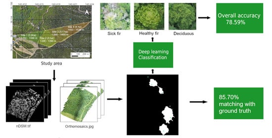
Insect outbreaks are a recurrent natural phenomenon in forest ecosystems expected to increase due to climate change. Recent advances in Unmanned Aerial Vehicles (UAV) and Deep Learning (DL) Networks provide us with tools to monitor them. In this study we used nine orthomosaics and normalized Digital Surface Models (nDSM) to detect and classify healthy and sick Maries fir trees as well as deciduous trees. This study aims at automatically classifying treetops by means of a novel computer vision treetops detection algorithm and the adaptation of existing DL architectures. Considering detection alone, the accuracy results showed 85.70% success. In terms of detection and classification, we were able to detect/classify correctly 78.59% of all tree classes (39.64% for sick fir). However, with data augmentation, detection/classification percentage of the sick fir class rose to 73.01% at the cost of the result accuracy of all tree classes that dropped 63.57%. The implementation of UAV, computer vision and DL techniques contribute to the development of a new approach to evaluate the impact of insect outbreaks in forest.

Graphical Abstract

1. Introduction

As a result of climate change, insect outbreaks are affecting forest ecosystems irreversibly around the world [1,2,3]. Since 2013, the Maries fir forests in Zao Mountain in Yamagata Prefecture, Japan have been subjected to insect-induced disturbances. Initially the tree defoliator, Tortrix moth (Epinotia piceae) infested trees affecting their capacity to perform photosynthesis. A second infestation of bark beetles (Polygraphus proximus) attacked the already weakened trees and led to extensive tree mortality [4,5,6]. This coniferous tree species has a high economic value for timber production but mainly as local tourist attraction because of the way snow accumulates on its branches, creating giant shapes known as “Snow Monsters”.
In recent years the use of Unmanned Aerial Vehicles (UAV) for the evaluation of forest health have significantly increased [7,8,9]. UAVs make data acquisition possible in areas where access is difficult [10], such as Zao mountain, where field studies face challenges due to unfavourable weather conditions and complex terrain. It also opens up opportunities to study mountainous natural forests where there are irregular tree distributions and high variability among individual tree characteristics (size, species, and position)- by reconstructing 3D images of the forest [11,12,13]. Furthermore, such data present high spatial resolutions (of up to centimeters per pixel) allowing for the analysis of single-tree-canopies [14,15]. Single tree identification is essential to classify trees, to monitor their health or to estimate forest inventory, forest biomass and carbon stocks among other forest characteristics [10,16,17].
Individual tree detection is a necessary step towards identifying sick trees and monitoring the spread of tree diseases in forest [7,9]. Many studies have detected individual trees and determined their health using different imaging modalities. Nasi et al. [7] detected single trees based on dense point cloud and hyper-spectral UAV images and classified “healthy” and “dead” trees in a bark beetle infested spruce forest. The study achieved 74% accuracy of detection and 90% accuracy of classification. Dash et al. [18] evaluated the health of mature plantation trees based on spectral indices of multi-spectral UAV imagery and obtained a classification accuracy of 70%. However, the study did not perform any result of tree detection. Sylvain et al. [19] mapped insect induced disturbances in forests using multi-spectral aerial images. No automatic tree detection algorithm was used in this study and instead an extremely large number of trees (around 290,000) were manually detected and classified to construct a ground truth dataset. They then annotated data and classified the trees using deep learning networks, obtaining accuracies of 96% for health status (dead and alive), 85% for plant functional type (broadleaf and needle) and 79% for a combined classification. Lidar data has also extensively been used for individual tree detection. Sun et al. [20] employed the Fusion software [21] for treetop detection in elevation models built using LIDAR data and then classified RGB patches corresponding to individual trees into 18 species obtaining 73.25% accuracy. However, in this case, the treetop detection step was not evaluated. A similar approach to data processing was followed in [22]. The elevation models built from Lidar data were combined with RGB imaging to train object detection networks to find individual trees in three different sites (a plantation forest, a sparse natural forest and an urban forest). Detection rates of 76.8% of existing trees were achieved using an ensemble strategy.
In contrast to classical computer vision algorithms, where general expert knowledge is used as an evaluation metric, emerging technologies such as Deep Learning (DL) allow for the incorporation of that knowledge into the automatic processing of the images. To build a DL network, first an architecture or set of nodes and connections among them is defined. The type of each node, the number of nodes and the connections between them, determine the behavior of the network. Subsequently, the network is given example data, the DL algorithm learns from these examples, known as training data. The data are run through the network and the weights in all the nodes are changed following an optimization process. The ways to solve the problems learnt by the computer are, thus, directly determined by the expert input. In natural forest, the specific tree characteristics that we want to find, are sometimes few in numbers, thus creating data imbalances for DL (which has been an important issue since the inception). For example, Dupret et al. [23] studied the amount of resampling needed to obtain the best results in binary classification problems using neural networks based on perceptrons. Their theoretical analysis showed how resampling can indeed improve the performance of classifiers and is most indicated when the cost of misclassifying one infrequent class is high in practical terms. However, the paper also states that the ratio between class samples needs to be carefully studied for each application. In recent years, the emergence of DL networks and their dominance in computer vision [24,25,26,27,28] has resulted in these ideas being revisited in light of new application opportunities and data resampling techniques such as data augmentation being widely used [29]. However, most of the existing approaches use data augmentation to improve classification performance in datasets that are small but balanced [30,31,32,33]. In particular, we quantify to which extent a careful use of data augmentation and the choice of an adequate DL architecture, can improve the detection of sick fir trees.
In relation to our current work, Onishi et al. [34], Natesan et al. [35] and Safonova et al. [9] used drone-acquired RGB data to develop algorithms for individual tree detection and classification in natural forests. Regarding the use of DL techniques to study forest health in UAV-acquired RGB images, Safonova et al. [9] used DL to recognize the degree of damage of fir trees in a natural forest. Onishi et al and Natesan et al. [34,35] used individual tree detection, in relatively small datasets, but the accuracy was not quantitatively evaluated in either work and only a qualitative evaluation was provided. Onishi et al. [34] worked with a total testing and training dataset made up of 941 tree images and achieved classification accuracies of 68-95% for the six species classified. Natesan et al. [35] worked with a dataset built by imaging one single site three times under different lighting conditions. This dataset contained 1786 tree images of three species and the authors used DL networks to achieve an average classification accuracy of 80%. Safonova et al. [9] first predicted potential regions containing trees in UAV images before classifying them into four degrees of pest infestation. The authors selected RGB images manually to build a balanced training dataset that was expanded using data augmentation. Non-tree containing parts of the orthomosaic were filtered out using computer vision processing. The highest accuracy was reported for dead trees at 91% without augmentation, while the lowest accuracy values were found for infested trees at 75%. None of these studies assessed the accuracy of individual tree detection results. To the best of our knowledge, only Diez et al. [11] quantitatively evaluated the tree detection algorithm by six different local maxima detection and image clustering algorithms
Consequently, we have identified two main issues using UAV-acquired RGB images to detect and classify individual trees in terms of their health or types. The first one is the relatively small datasets used in most studies so far. The second is the lack of attention on the performance of treetop detection algorithms when used in conjunction with classification algorithms. This is especially relevant for natural forests where tree detection is more challenging [11].
With this study we aim to contribute with a new methodology to evaluate insect infestation in forest using UAV-acquired images. Thus the objectives of this study are (1) Developing an algorithm capable of detecting treetops and evaluating its performance and (2) Applying DL networks to classify two different health conditions of Maries fir trees: (i) healthy and (ii) sick trees and a further class for (iii) deciduous trees. All the data and annotations used for this study are available at: https://doi.org/10.5281/zenodo.4054338. The source code is also available on demand from the authors.

2. Methodology

2.1. Study Sites, Data Acquisition and Problem Definition

2.1.1. Study Sites

The study sites are located on Zao mountain, a volcano in the Southeastern part of Yamagata Prefecture (38°09′10.5″N 140°25′18.4″E). The site covers an area of 18 ha with a tree density of about 200 trees/ha. The fir trees in the areas are between 41 to 103 years old with an average age of 72 years. We divided the image acquisition area into four sites using the small paths within the study area as dividing boundaries. These were used to distinguish both the forest composition and the degrees of insect damage along an elevation gradient. The elevation increases from 1250 m in site 1 to 1538 m in site 4. The sites have varying intensity of forest damage as well as compositions in terms of tree species—Site 1 (3.9 ha) and site 2 (5 ha) are composed of Maries fir mixed with other natural deciduous species such as: Acer ukurunduense, Fagus crenata, Sorbaria sorbifolia, and Salix. In sites 3 (5.1 ha) and 4 (4 ha), fir is the dominant species. Fewer sick firs are observed at the lower sites while the most severely damaged trees are found at higher sites. On the top of the mountain (1551–1706 m), all fir trees are already dead. Since our study focuses on the detection of sick trees, we exclude the top of the mountain and present results related only to sites 1 to 4 (Figure 1).

2.1.2. UAV Data Acquisition

Sets of RGB aerial photos were collected during the summer of 2019. Three flying missions in site 1 (mission 1,2,3); three in for site 2 (mission 4,5,6) and two in site 3 (mission 7,8) were taken with a DJI Mavic 2 pro Hasselblad L1D-20c camera. The drone acquired 20 Megapixel images, following routes designed on DJI GS pro software (DJI Inc., Shenzhen, China). The camera sensor is a 1 inch CMOS with fixed focal length 10 mm and aperture f/3.2. The weather on the capturing days varied but often entailed strong sun in the morning, then cloudy and windy in the afternoon. The drone flew at 70 m altitude from take-off points, nadir view, 3 m/s and shutter interval of 2 s. The photos were acquired with 90% side and front overlap. The camera was set at S priority (ISO-100) with shutter speed at 1/240–1/320 s when it was strong sun and windy and at 1/80–1/120 in more favourable weather conditions. These set-ups maintained exposure values (EV) around 0 to +0.7 providing a ground sampling distance (GSD) from 1.5–2.1 cm/pixel. We had one flying mission in site 4 (mission 9) used a DJI Phantom 4 Quadcopter. The camera sensor in this UAV is 1/2.3 inch CMOS with fixed focal length of 24 mm. The drone was pre-programmed to fly at 45 m high from take off point on a mild weather day. Photos were taken with 90% front and side overlap. The drone flew at speed 2 m/s, with a shutter interval of 2 s. The camera was set in automatic mode at a shutter speed of 1/120 s, ISO-100, EV at 0. This set up resulted in a GSD of 2.6 cm/pixel. The number of RAW images of each flight mission ranged from 150 to 390. All the photos have GPS coordinates which assist to 3D reconstruction.

2.1.3. Problem Definition

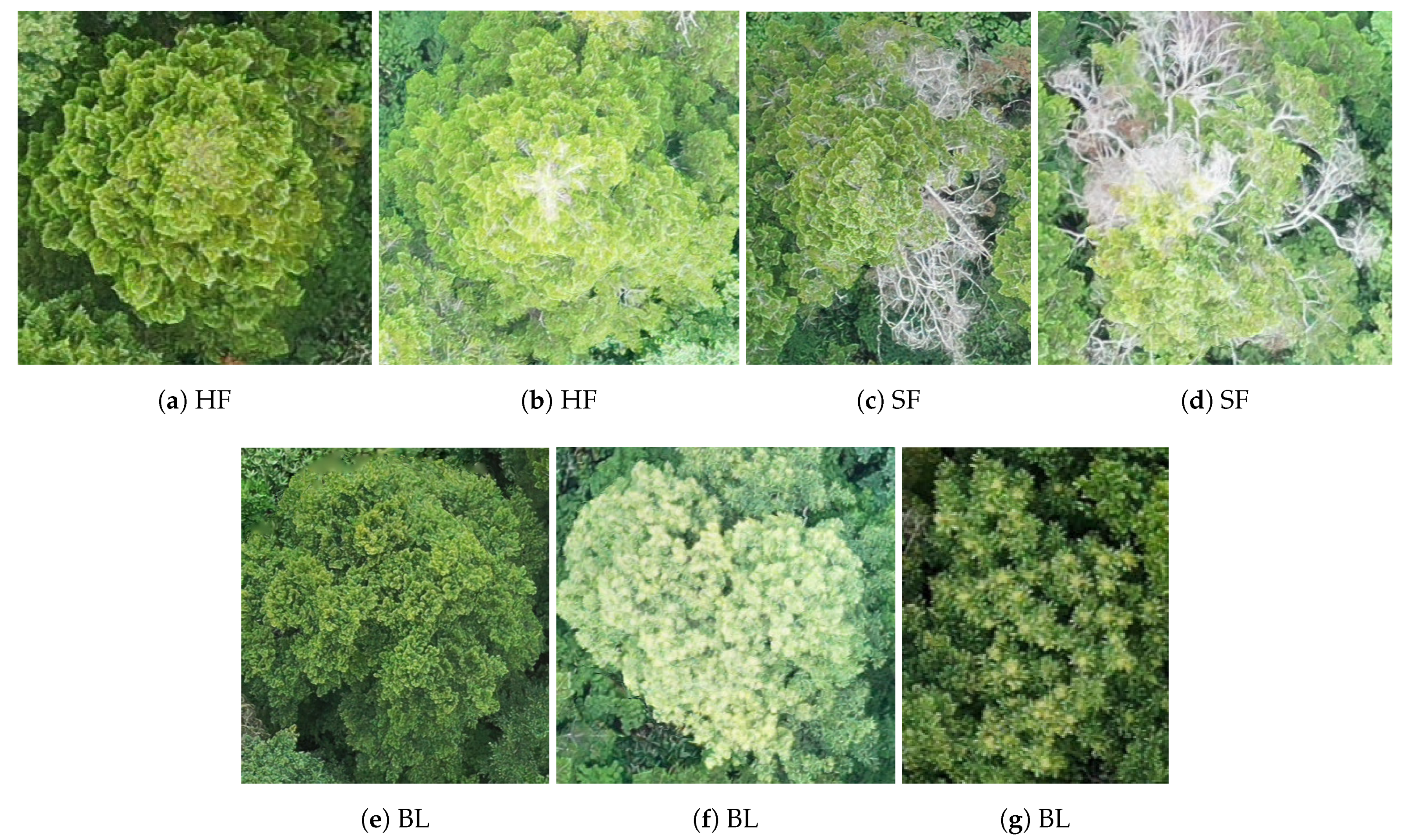
We divided the trees in our study area into three classes: sick fir (SF), healthy fir (HF) and broadleaf (BL) trees (hereafter HF, SF and BL). Pest infestation has different effects on individual trees, some trees show defoliation on lower branches while in others, defoliation appears on the top branches. In order to facilitate the classification, we followed the reference on crown condition classification of the USDA [37] in which the authors classified trees based on their defoliation rates. Following this classification, we subdivided fir trees in Zao mountain in two classes: healthy, when no leafless branches were observed and sick, when leafless branches were observed (Figure 2). Although there are several different broadleaf trees, especially on site 1 and 2, we classified all of them in the single class, BL (Figure 2).

2.1.4. Dense Point Cloud, DSM and Orthomosaic Generation

A Dense point cloud is a set of millions of points positioned by GNSS (Global Navigation and Satellite System) with 3 dimensional locations (x,y,z). It is used to generate the DSM and the orthomosaics. A DSM contains the altitude information of each pixel to the earth datum and provide a validation tool for nDSM (see Section 2.2.1) in our study. Orthomosaic images are composed of all raw single images of each flight and are geographically corrected to be at the true position, reducing the distortion from camera, lens and topography. An orthomosaic facilitates the labelling of trees in order to create the training and testing patches for DL. In this study, dense point clouds, DSM and orthomosaics were generated after aligning the raw RGB images of each flight using Agisoft Metashape [38].
The dense point cloud, DSM and orthomosaics were created in Metashape using batch procedure for the whole dataset of each flight. First each set of RGB images was aligned without ground control points (GCP), accuracy to highest, 40,000 key point limit and 0 tie point limit were set. Then the “optimize alignment” step was set to default. In the next step the “dense point cloud” (high quality, aggressive filtering), “mesh” and “texture” were built. The procedure was completed with DSM (interpolation enable) and orthomosaics (surface = DSM, blending mode = mosaic, hole filling = yes). All the dense point cloud, DSM and orthomosaics were exported to Tokyo UTM Zone 54N. The same pixel size and extent were set for DSM and orthomosaic of each flight to overlay and process them in GIMP [39] and Python [40].
This is the first step that will be followed by nDSM generation, treetop detection, treetop classification and finally the validation of the results (Figure 3).

2.2. Data Pre-Processing

2.2.1. Normalized Digital Surface Model (nDSM) Generation and Validation

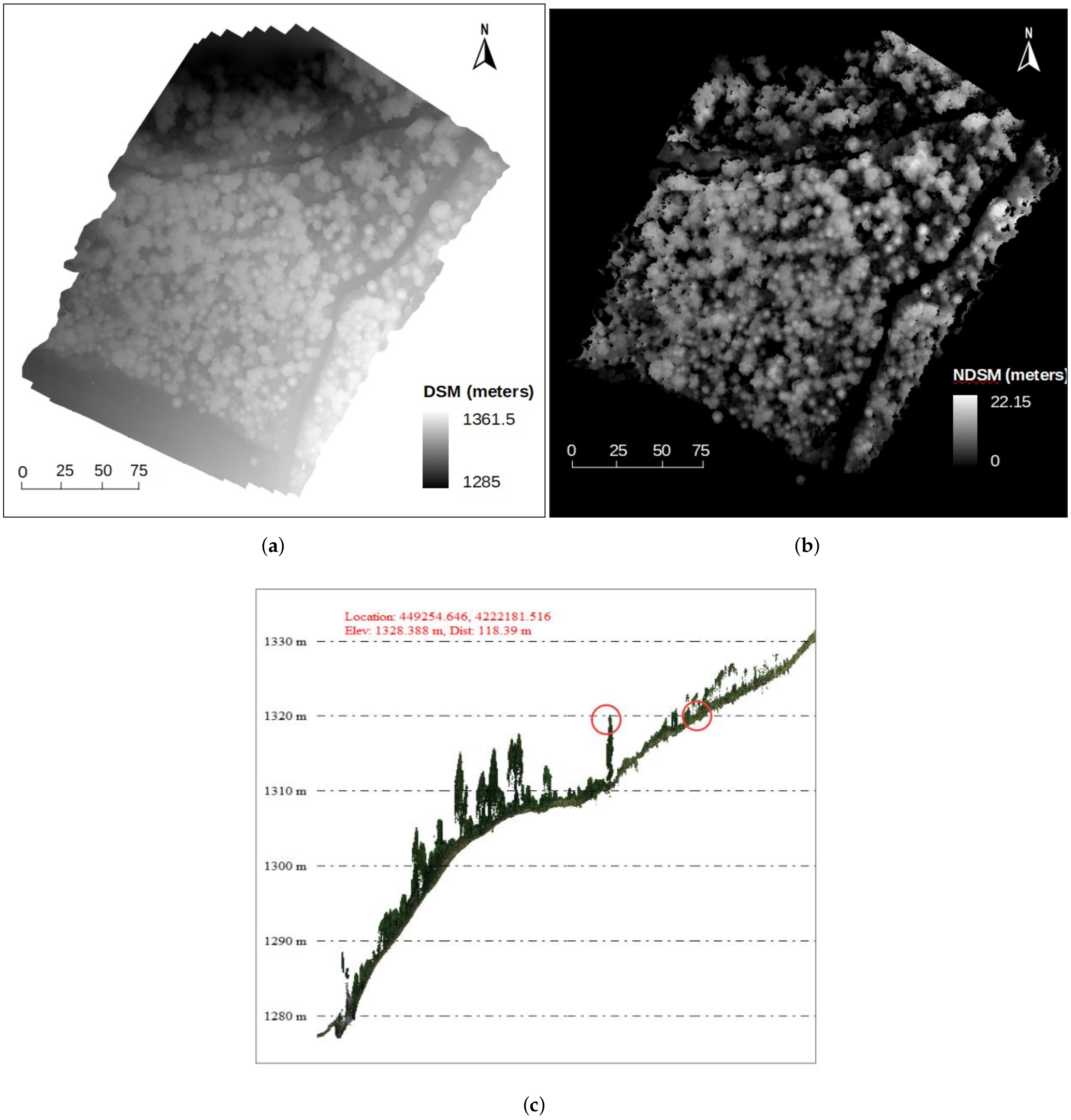
An nDSM is an elevation model represented on a 2D digital grid surface to display the elevation of all features above the ground. It was generated in order to filter out the forest floor and produce elevation maps that only contained the height of trees (Figure 4). An nDSM was created by subtracting the Digital Terrain Model (DTM) from the dense point cloud, where the Digital Terrain Model (DTM) is an elevation model of bare-earth on a raster image. Our treetop detection algorithm is based on the local maxima method, therefore, if we use DSM for treetop detection in steep slopes, the highest point (treetop) downhill could be at the same altitude of the forest floor uphill (Figure 4). However, when we use nDSM, the local highest points are only the treetops as the forest floor is already normalized (removing the slope effect).
In order to generate nDSM we followed several steps: Fusion/LDV [21] was used to define bare-earth points with the function “GROUNDFILTER” adapted from the filtering algorithm of [41]. Then the bare-earth points were converted to plane surface digital terrain model (DTM) 0.2 m cell size with the function “GRIDSURFACECREATE”. This function fitted the surface to the forest floor that was visible and interpolated the parts that were not visible under the canopies. The DTM was subtracted from dense point cloud with function “CLIPDTM” to generate the normalized dense point cloud and then the terrain was normalized to 0 m. Next, the software Global Mapper [42] was used to filter the points lower than 2 m (considered as lower vegetation) and points that belong to artefacts. The filtered points were then converted to nDSM where only tree canopies were present, with the same pixel size as that of the orthomosaic (about 0.02 m) of the same area. Finally, QGIS [36] was used to convert data from tiff to jpg format for image annotation with GIMP (GNU Image Manipulation Program) [39] software.
In order to perform a detailed evaluation of the results of this pre-process we would need a highly precise digital elevation model, such as the one that could be obtained with a ground based LiDAR system as well as detailed 3D annotations separating the section of the tree models corresponding to tree canopies. As such a model was not available, we focused on the visible effects that the nDSM construction step had on our ground truth. Specifically we annotated the treetops manually on the DSM and then monitored how many of them were left out from the nDSM. A treetop was defined to be left out of the nDSM if (a) it was on a black pixel value (removed area) or (b) it had not been assigned a black value but the connected component it belonged to was smaller than a predefined threshold.

2.2.2. Data Annotation

Annotation is a data preparation step where all trees are manually labelled on orthomosaic images into different binary layers (black and white). GIMP, open source software for photo-editing was selected to manually label the tree categories. Additionally, treetops were annotated on the DSM and nDSM in order to first, verify if all the treetops were also found on nDSM and second to evaluate the result of the treetop detection algorithm (Section 2.3). The treetops were manually labelled by marking black dots at the highest area of every tree in GIMP.

2.3. Treetop Detection

2.3.1. Treetop Detection Algorithm

This section describes the algorithm that was used to detect treetops in nDSM data. In order to take full advantage of the precise data representation obtained with the nDSM, a geotif data format with float components was used, allowing us to encode altitude values in millimeters. The algorithm uses computer vision techniques to find the regions in the nDSM that correspond to the tips of the treetops. A sliding window is used to process small parts of the nDSM independently. First, at each window position only the pixels with higher intensities are considered. Then wider ranges of intensities are added iteratively. In each new iteration, connected components not containing any previously detected treetop are considered and if their areas are large enough, new treetops are assigned to them. The process continues within the window until all pixel intensities are taken into account. Subsequently the window is shifted to a new location. Once all the positions of the sliding window have been explored, a refinement step is performed to join nearby candidate treetops.
Details of each step of the algorithm are as follows:
  • Two-step algorithm: a large concentration of treetops at the higher intensity pixels was observed, for example in the first orthomosaic 50% of the treetops are contained in the 10% higher pixels and 90% of the treetops are contained in the 40% higher pixels. Consequently, the algorithm runs in two main steps (which we refer to as “bands”). The first considers only pixel intensities of the nDSM from a certain threshold up and the second one considers all intensities.
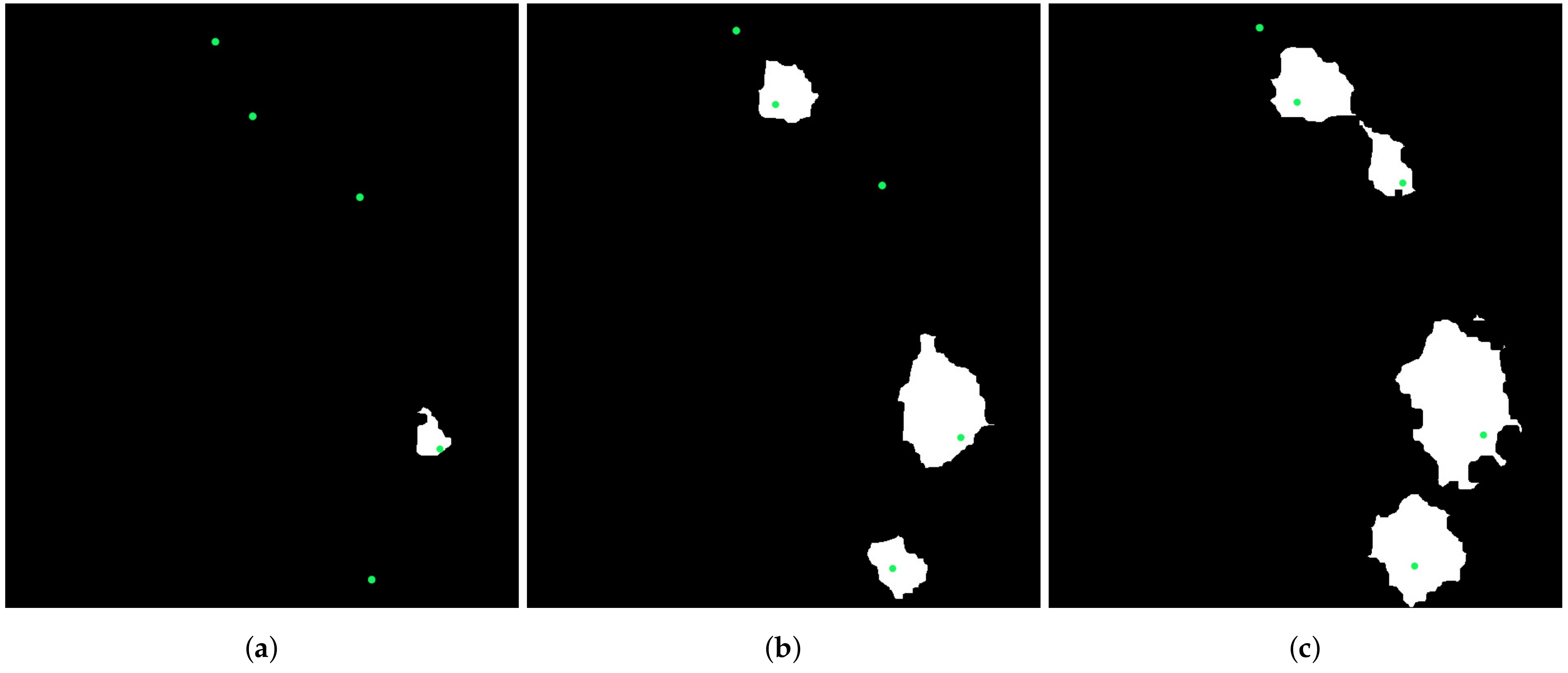
  • Sliding window: for each of these two steps, a sliding window is passed over the nDSM. The positions of the window have a 100-pixel overlap. For each position of the window (Figure 5), a list of candidate treetops is initialised to an empty list and a threshold value t h is set. Then at each iteration:
    • Only the upper band of intensities (larger than t h ) is considered.
    • Connected components are computed in the image limited to the current window and band of pixel intensities. Each newly appearing component (if it is large enough) is assigned a new treetop that is added to the list of treetop candidates. Connected components already containing a candidate treetop do not add new candidate treetops to the list. If two connected components contain one treetop then they are fused and both treetops are kept.
    • t h is updated and the process continues until t h reaches the minimum intensity present in the window.
  • Refinement: once all the treetops are computed, they are refined to eliminate those that are too close to each other, specifically, a circle is drawn around each candidate treetop (with radius r e f R a d = 50 pixels) to exclude pixels higher than the candidate top (with a difference of more than 1.5 meters with the top). Then, the top point in each of the connected components is chosen as a predicted treetop. Thus, the highest treetops among those whose regions intersect are selected and the lower are discarded. An initial refinement step is done over the candidate tops resulting from considering all pixel intensities. Then, the treetop candidates corresponding to the high intensity bands is performed. As the treetops detected in the higher-intensity band are considered more reliable, this second refinement step is less strict (the value for r e f R a d = 35).
Figure 5. Green pixels contain the real treetops, white pixels contain the mask of the part of the nDSM that is being considered. For each position of the sliding window, only the top intensities are considered (step 1). Every time a new connected component appears, its area is considered. Is the area is large enough, a treetop is predicted in the pixel with higher intensity. Subsequently, a widening range of intensities is taken into account and the connected components not yet containing predicted treetops are considered. In (a) step 1, one fir tree is detected, (b) in step 2, two more are detected and finally (c) in step 3, one more is detected.
Remotesensing 13 00260 g005

2.3.2. Treetop Detection Validation

In order to evaluate the quality of the results of the treetop detection algorithm we defined five different criteria. The output of the treetop algorithm is a set of points given in the form of a list of 2D (x,y) coordinates. Consequently, all of these criteria considered two sets of 2D points: the set of predicted points as well as the set of manually annotated ground truth points.
Average Euclidean distance to nearest ground truth point ( d E u c ( P R E D , G T ) ): this criterion aims to measure how close the treetops predicted are to the ground truth points. It is calculated as the average of all Euclidean distances between every ground truth point p ¯ to its nearest predicted point p ^ .
d E u c ( P R E D , G T ) = p ^ P R E D m i n p ¯ G T d ( p ¯ , p ^ ) | P R E D |
This metric, however, is somewhat vulnerable to outlier points skewing the value. Also, it does not clearly express how many predicted points are “close enough” to ground truth points. Consequently, two other metrics were provided.
Matched ground truth points percentage (m%): the aim of this metric is to provide an indication of how many treetops were detected. In order to implement this, a value was considered that roughly represented the radius of a tree crown ε . Predicted points were considered “matched” if they were within this threshold of a ground truth point ( d ( p ¯ , p ^ ) < ε with p ^ P R E D and p ¯ G T . After carefully examining the trees in the orthomosaic a distance of approximately ε = 2.5 meters was used as the permissible margin of errors for two points to still be considered as the same tree crown. Given the differences in pixel resolution between sites 1, 2 and sites 3, 4, this stood for an error margin of 125 pixels for sites 1, 2 and 100 pixels for sites 3, 4. This set of thresholds make our use of this metric highly restrictive in terms of larger tree crowns which can be up to eight meters in diameter and we would only be considering a small part as valid for matching. However, we chose them to make it very difficult for a point predicted in one tree crown to be matched to a ground truth point in a neighbouring tree crown even in the case of small trees (whose diameter is typically closer to 3 m). This addresses the issue of whether the points detected are placed correctly. However, during our experiments we realised that methods providing a large number of candidate points obtained high values for this metric that did not agree with the subjective evaluation. Thus, in order to complement this metric, a simple metric based on the difference between the number of ground truth points and the number of detected points was provided.
Average Euclidean distance to closest ground truth points (correctly identified trees only): a combination of the two previous criteria, the goal in this case is to focus on the quality of the detection of correctly identified points.
Counting measure (cnt %): stands for the difference of trees present in one nDSM “n”, with the number of treetops detected “k” weighted over the number of trees c n t = n k n . Consequently, negative values indicate that the algorithm overestimated the number of trees, while positive values indicate underestimation. While reporting averages each absolute value was taken to prevent that these two errors cancel each other.
Percentage of ground truth points detected more than once: to complement the counting criterion, we also computed the percentage of ground truth points that were matched more than once. This criterion provided us with more detail into the source of prediction overestimation A higher number in this criterion indicated a difficulty to separate individual treetops while a lower number indicated erroneous points being detected in outer parts of tree canopies.
In order to provide a full picture, the results of the algorithm were compared to those of three previously existing methods. First, two methods (clustering and extrema-based methods) [11], were used to exemplify the two families of approaches. Results for iterative Global Maxima GMax and Gaussian Mixture Model clustering GMM are, thus, presented. Additionally, results regarding the treetop detection method in [9] are also provided. This method, unlike the method in our study, works using the RGB orthomosaics to detect treetops. First, the orthomosaics are transformed into grayscale and blurred, then a thresholding step is used to work with binary images. The resulting images are then eroded and dilated repeatedly to isolate individual trees and finally a contour area calculation function is used (Dawkins implementation) to determine treetop candidates. We followed the execution of this algorithm with an additional step where predicted points that were identified as ground in the nDSM were eliminated.

2.4. Treetop Classification

In order to capture the distinctive characteristics of each tree type, a small square patch (100 × 100 pixels approximately 2 × 2 sq.m) around each treetop was sampled (indicated by a single point at its center). Then, each patch was assigned a class according to the manual annotation codifying the classes that could be found in the image (SF, HF and BL). Using this information, the problem was formalized in terms of DL as a classical single-label classification problem using the patches extracted around the treetops. This problem was solved using one of the following DL classifiers:

2.4.1. Treetop Classification Algorithm

In order to classify the patches representing each of the detected treetops, a series of feature extractor DL networks was used. The following architectures were considered as defined on the FastAI Library [43]. This library uses the torchvision package from pytorch (A description of the implementation of each model and a quantitative comparison on the ImageNet dataset can be found at https://pytorch.org/docs/stable/torchvision/models/).
  • Alexnet [24] is one of the first widely used convolutional neural networks, composed of eight layers (five convolutional layers sometimes followed by max-pooling layers and three fully connected layers). This network was the one that started the current DL trend after outperforming the current state-of-the-art method on the ImageNet data set by a large margin.
  • Squeezenet [25] uses so-called squeeze filters, including point-wise filter to reduce the number of necessary parameters. A similar accuracy to Alexnet was claimed with fewer parameters.
  • Vgg [26] represents an evolution of the Alexnet network that allowed for an increased number of layers (16 in the version considered in our work) by using smaller convolutional filters.
  • Resnet [27] is one of the first DL architectures to allow higher number of layers (and, thus, “deeper” networks) by including blocks composed of convolution, batch normalization and ReLU. In the current work a version with 50 layers was used.
  • Densenet [28] is another evolution of the resnet network that uses a larger number of connections between layers to claim increased parameter efficiency and better feature propagation that allows them to work with even more layers (121 in this work).
All these DL classifiers were initialized using Imagenet weights [24] with their final layers substituted by a linear layer with our number of classes. This final layer was followed by a sofmax activation function.

2.4.2. Data Augmentation

Data augmentation is a commonly used strategy in DL that allows to increase the size of datasets without the need to collect new data. In our case, SF is the most important category. However, this category is much less frequent than the other two. In order to increase the relative weight of sick fir trees during the training process of DL networks, we used six image transformations to augment our data: up/down and left/right flips, small central rotations with a random angle, Gaussian blurring of the images, linear and small contrast changes and localised elastic deformation. To implement these transformations we used the “imgaug” library [44].

2.4.3. Treetop Classification Algorithm Training and Validation

The treetop classification algorithm received input of treetop points. For each of these points, the algorithm:
  • Checked to which of the classes it belonged.To do so it checked the manually annotated class binary masks (See Section 2.2 for details on the annotation process).
  • Cut a small patch of the orthomosaic around each treetop (of 100 × 100 RGB pixels, amounting approximately to a 2 m sided square).
  • Once the correct class had been identified and the patch built, the patch was stored as an image with the class name in its file name.
The set thus constructed was then passed on to a deep learning network where it was divided into training/validation and testing subsets. The treetop points used to build the sets as well as the way the training/validation/testing subdivision was made determined what was being tested. Regarding the treetops, first we used the ground-truth treetops annotated by experts in order to assess the performance of the classification algorithm with the best possible input data. Then we used the output of the tree detection algorithm to assess how the classification algorithm performed as a part of the whole algorithmic pipeline presented (see Section 3.4). Regarding the division in validation and testing, first we used all data from all mosaics in a single dataset, dividing it randomly in 80% training/validation and 20% testing. However, as mosaics in the same sites have overlap, images from the same tree (taken in different mosaics and thus, in different flights with different lighting conditions) might have appeared in both the training and testing sets.
We considered this a problem as it put into question the generalization power of the classification algorithms. Consequently, we also used (in both experiments) a site-based leave-one-out strategy to prevent this issue as follows:
The orthomosaics available were grouped into sites, all the mosaics of three of the sites were used for training/validation while all the mosaics of the remaining site were used for for testing. The site used for testing was rotated so all orthomosaics were used for testing once and no orthomosaic was used for training/validation and testing at the same time to avoid leakage between the training and testing patches.
  • First fold, testing: Site 1 (mosaics 1,2,3) training/validation Sites 2,3,4 (mosaics 4–9)
  • Second fold, testing: Site 2 (mosaics 4,5,6) training/validation Sites 1,3,4 (mosaics 1–3,7–9)
  • Third fold, testing: Site 3 (mosaics 7,8) training/validation Sites 1,2,4 (mosaics 1–6,9)
  • Fourth fold, testing: Site 4 (mosaic 9) training/validation Sites 1,2,3 (mosaics 1–8)
In all cases, the following measures were used to evaluate the classification accuracy:
In order to target the predictive capacity of the algorithms the relation between predicted values and ground truth values was considered and expressed as: True Positives ( TP), False Positives (FP), True Negatives (TN), False Negatives (FN). Furthermore, and in order to focus on the defined classes, the following measures were computed on them: True Positive Rate (TPR), also known as Sensitivity (SENS), False Positive Rate (FPR), also known as the probabilistic complement of Specificity (SPEC) and finally accuracy (ACC). Their formulae as follow:
T P R = S E N S = TP TP + FN F P R = 1 S P E C = FP TN + FP A C C = TP + TN TP + TN + FP + FN

3. Results

3.1. nDSM Validation

nDSM validation (Table 1) was expressed as the percentage of ground truth treetop found in the DSM missing in the nDSM (0% means all ground truth treetops are present) (Table 1). The percentage of treetop missing in nDSM6 and nDSM4 were 0.0% and 6.9%, representing the lowest and highest values respectively. The mean validation value of all the nDSM was 2.14%
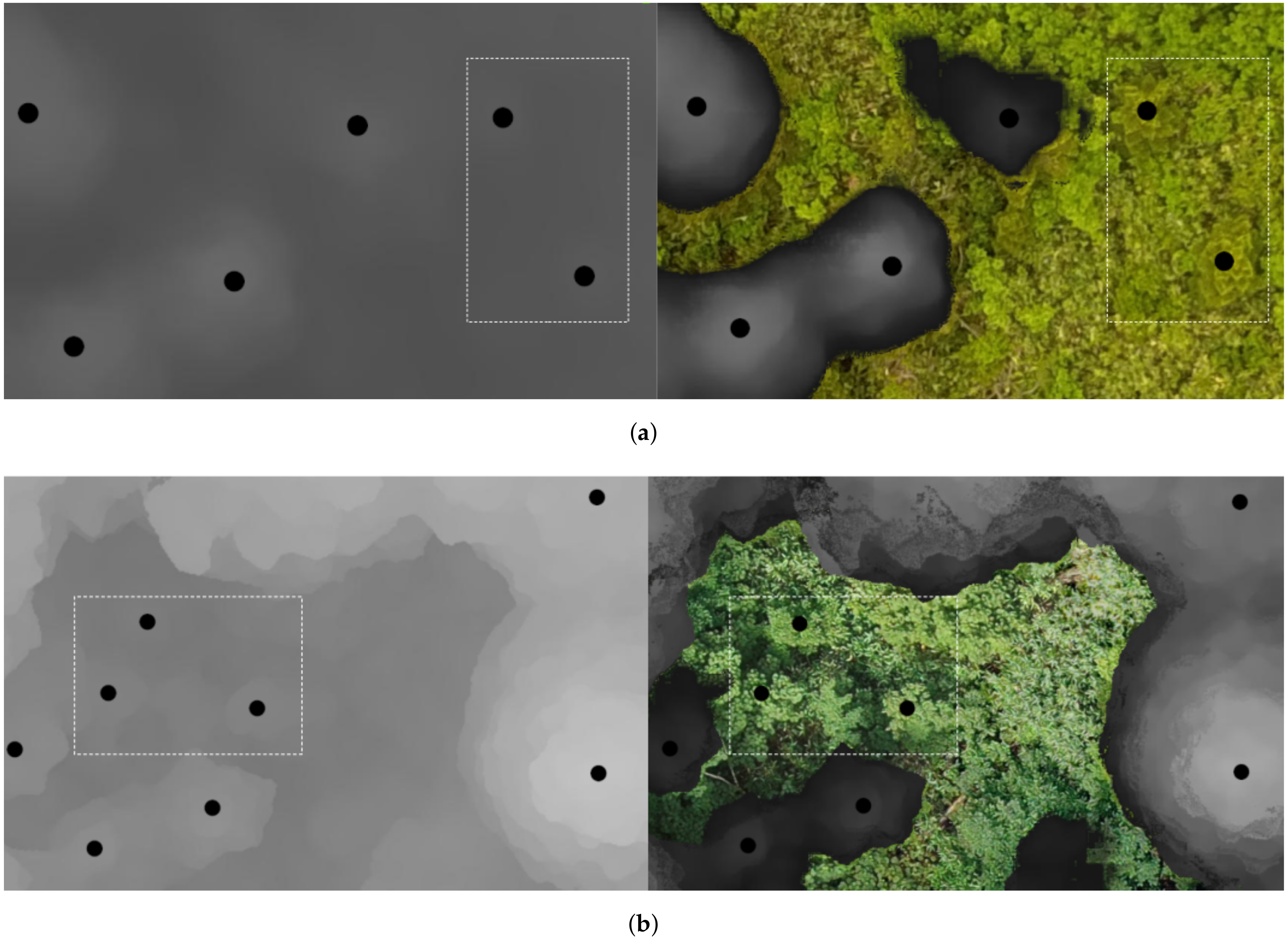
After a visual review of the images, we found that most of the annotated treetops missing were those of smaller deciduous trees in distorted areas of the orthomosaic boundary or were small fir trees (2–6 years old) (Figure 6). Missing trees represent one of the limitations of this study, since only the treetops found in the nDSM are considered.

3.2. Treetop Detection

The performance of the treetop detection algorithm introduced in Section 2.3 was evaluated using the quality criteria and comparing it with the results of three pre-existing algorithms [9,11]. The percentage of points matched (m%) and counting measure (cnt) obtained by each of the algorithms in each of the nDSM (Table 2).
The results showed that the method introduced in this paper obtained the best overall results both in the matching (85.70%) and counting (9.67%) criteria. Differences in the results depending on the nDSM, for example nDSM 1,3 and 9 showed higher accuracy in treetop detection ranging form 89.61% to 96.29%, while nDSM 5 and 6 obtained matching values around of 85%. The lowest values were obtained for nDSM 2,4,7 and 8 but still were all in the range of 80%. The lower matching averages were observed in nDSM that corresponded to lower and middle areas with steep slopes and the highest rate of mixing with decidous trees.
Regarding the counting criterion, our algorithm tended to slightly over-estimate the number of trees that are represented by cnt negative values. This over-estimation was kept, however, under 10% for most of the orthomosaics and with less variability as that found when using the other methods. The methods based on finding local extrema and on clustering algorithms GM and FCM obtained lower performances for matching with values around 71% and similar performances in terms of the counting criterion. The Dawkins method used before in [9] obtained poor results in terms of matching percentage with an average of 66.02% with some very low performances in the lower and middle elevation sites (around 50% for nDSMs 2,5,6) and very good performance for the nDSM in the highest elevation site (nDSM 9).
Regarding other metrics using our method, the average Euclidean distance between the sets of predicted and ground truth points, obtained the best value with an average of 50.29 pixels of distance (around 1 m) between each predicted point and its closest ground truth point. As this also considered unmatched points (further than 100 or 125 pixels) it illustrates the strength of the presented algorithm. The values for this criterion obtained by the other methods were: FCM 116.32, GMax 118.11, and Dawkins 178.67). The quality of the matching results is also compounded when we consider the euclidean distance for correctly matched points only. The distance drops from 50.29 to 27.42 showing how points correctly found in canopies were on average about 50 cm from their corresponding ground truth point. The percentage of points detected more than once was on average 8.22% with the highest value of 15.68% for orthomosaic 1 which had the highest occurrence of deciduous trees.

3.3. Classification of Ground Truth Treetops Using Deep Learning

In this experiment we assessed the capacity of the DL networks to classify treetops into the healthy fir, sick fir and deciduous classes. In order to focus on the merits of the classification algorithms, manually annotated treetops were used (from now referred to as ground truth or GT treetops).
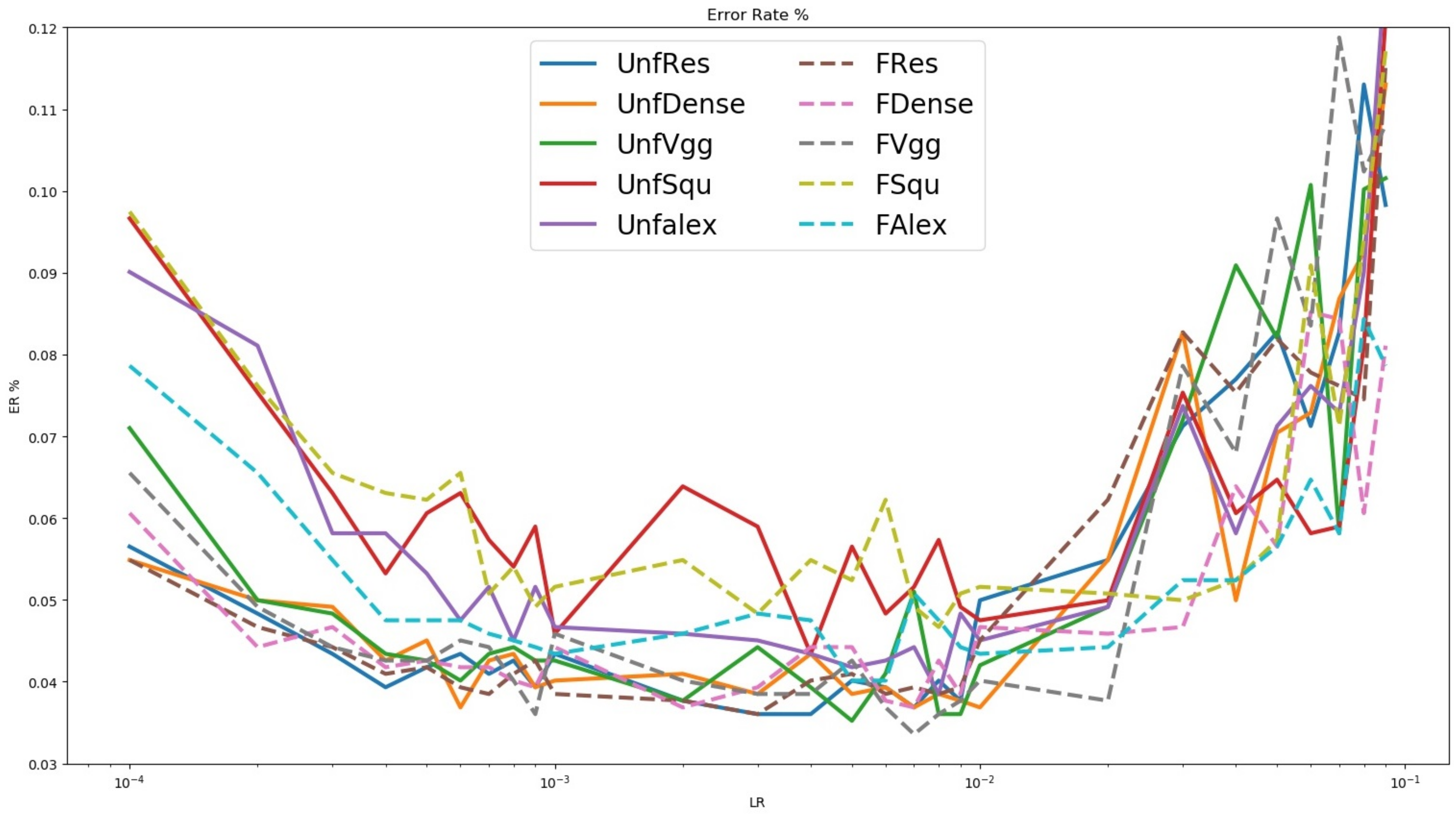
The data remaining inside the chosen Region of Interest (ROI) of the 9 orthomosaics in the 4 sites contained 5364 trees (1407 deciduous, 3788 healthy fir and 169 sick fir). Initially, the dataset constructed considering patches corresponding to all these treetops was divided randomly into 80% training and 20% testing. Figure 7 contains the percentage of misclassification over all images (Error Rate, ER) values for the validation set in each of the considered DL architectures over a list of learning rate values.
The most suitable results were obtained by Vgg, with the highest ER value of 0.03357% for FVgg and learning Rate (LR) = 0.007 (Figure 7). The same network reached 0.03521% ER in its unfrozen version (UNFVgg, LR = 0.005). Resnet and Densenet obtained similar results (0.03603% UNFResnet, LR = 0.004 or 0.03685% UNFDense, LR = 0.007) with small difference between their frozen and unfrozen versions. Alexnet and Squeezenet obtained the lowest results with Alexnet doing slightly better with just under 0.040% ER (0.03949% for UNFAlex LR 0.008) and Squeezenet reaching an ER of 0.0434% (UNFSqu, LR = 0.004). These results show that all networks are successful at classifying the images received into the three existing classes. However, the results obtained presented problems in terms of their practical use: the class with the highest interest was sick fir trees. However, most of the networks produce low specificity value for this class. Table 3 shows the best results obtained regarding this criterion together with the specificity, sensitivity and accuracy of the other classes (Densenet LR = 0.06).
Table 3 shows that even though high accuracy results were obtained in the three classes, the sick fir class obtains very low results in its sensitivity value. This stands for the classifiers miss-classifying about half of the sick fir images. The fact that this class is less frequent than the other two accounts for the high accuracy obtained regardless of this.
Furthermore, the data used in this section contains images from all orthomosaics and sites. Since, the orthomosaics contain an overlap of the adjacent site (1,2,3 for site 1, 4,5,6 for site 2, 7,8 for site 3 and 9 for site 4), it is possible that the validation sets contained images of trees that also appear in the training set. While this is often seen in the literature due to the difficulty of obtaining data, we assume that training the networks in this manner may contribute to a subtle form of over-fitting. In order to obtain a classification algorithm that presents improved sensitivity for the sick fir class, we used data augmentation and a leave-one-out strategy for the building site-specific training sets.
In terms of DL networks and given the results presented here, our focus was set on the Unfrozen version of the Vgg, ResNet and DenseNet. While the best performances of Frozen and Unfrozen networks were very similar, the smaller variance of Unfrozen networks were valued as a sign of a more stable performance and were considered as being better suited for the use of data augmentation because of the larger number of modifiable parameters.
This is expected to increase the classification accuracy of the images containing the augmented classes at the cost of decreasing that of the other classes. To avoid having images of the same tree (even if taken in different flights) both in the training and testing set we used a site-based leave-one-out strategy and build one training/validation distribution of images for each site.
In short, in each fold of the leave-one-out, the orthomosaics of one site were used as the testing set, while the orthomosaics of all the other sites conformed with the training set. The sensitivity, specificity and accuracy for the 4 sites using the three DL networks considered (Densenet, ResNet and Unfrozen Vgg) and five different data augmentation scenarios: No augmentation (row “no augm” ) and 2,6,10 or 20 augmented images for each original sick fir image (rows augm 2 to augm 20) were used (Table 4).
The results show that the use of data augmentation led to better sensitivity values for the sick fir class. Although a decrease in specificity was observed due to an increase in the number of False Positive detections of the sick fir class, the classification accuracy of this class grew. This is mainly due to the relatively low number of sick fir trees compared to the total number of trees (sick and healthy fir plus deciduous). Comparing the three networks studied, Vgg obtained slightly lower values with Densenet and Resnet showing similar values. In order to choose between the two networks the average specificity, sensitivity and accuracy values were analyzed in all the learning rates considered, obtaining, for example for augm10, values of 0.8781, 0.97632, 0.9532 for Densenet and 0.8908, 0.9758, 0.9558 for Resnet. Even though the differences remained small, Resnet obtained higher values for all datasets suggesting a more stable behaviour in this classification problem. The same indicators for the other two classes (healthy fir and deciduous) showed similar tendencies. For example, for the same dataset (augm10) and comparing the two learning rates with better sick fir specificity values, Resnet (LR = 0.001) obtained values of 0.9830, 0.8953, 0.9601 for healthy fir, and 0.9720, 0.9921, 0.9877 for deciduous while Densenet (LR = 0.006) obtained 0.9431, 0.8790, 0.9225 for healthy fir and 0.9548, 0.9601, 0.9586 for deciduous. These values illustrate the slightly superior performance of Resnet over Densenet as well as the trade-off between the larger specificity values for the sick fir class and a decrease in percentage for the other classes. The use of data augmentation increased the impact of the sick fir class in the training step. This results in better specificity for it but also increases the number of False Positives in the healthy fir class. Considering these results, the Resnet network was used to classify treetops detected automatically using the algorithm introduced in Section 2.3.

3.4. Automatic Detection and Classification of Sick Fir trees

Finally all the algorithms presented in this paper were used together and their combined performance was evaluated. First, the pre-processing procedure was used to obtain a nDSM from the drone-acquired data. This nDSM was then used as input for the treetop detection algorithm and as a result, a list of ( x , y ) coordinates representing the position of each automatically detected treetop was obtained. The treetops thus detected were then classified into the three existing classes (SF, HF and BL) using the Resnet network.
Regarding the training/testing sets, used for the Resnet classifier network, the site-wise leave-one-out approach was used. Within each fold of the training set, we initially used the exact same approach as in Section 3.3, where ground truth treetop points were considered and 100 × 100 pixel images were cut around them (approximately 2 × 2 sq.m). The testing set was then built by cutting 100 × 100 pixel images around the automatically detected treetop candidate points. However, the results of this approach were not satisfactory, mainly because on the training set the trunk of the trees was always placed at the center of the image whereas in the testing set this was not always the case. In order to ameliorate this problem we considered small perturbations of the coordinates of the ground truth points so that the generated 100 × 100 pixels were not perfectly centered on the actual ground truth points. All the results presented in this section all correspond to this training strategy.
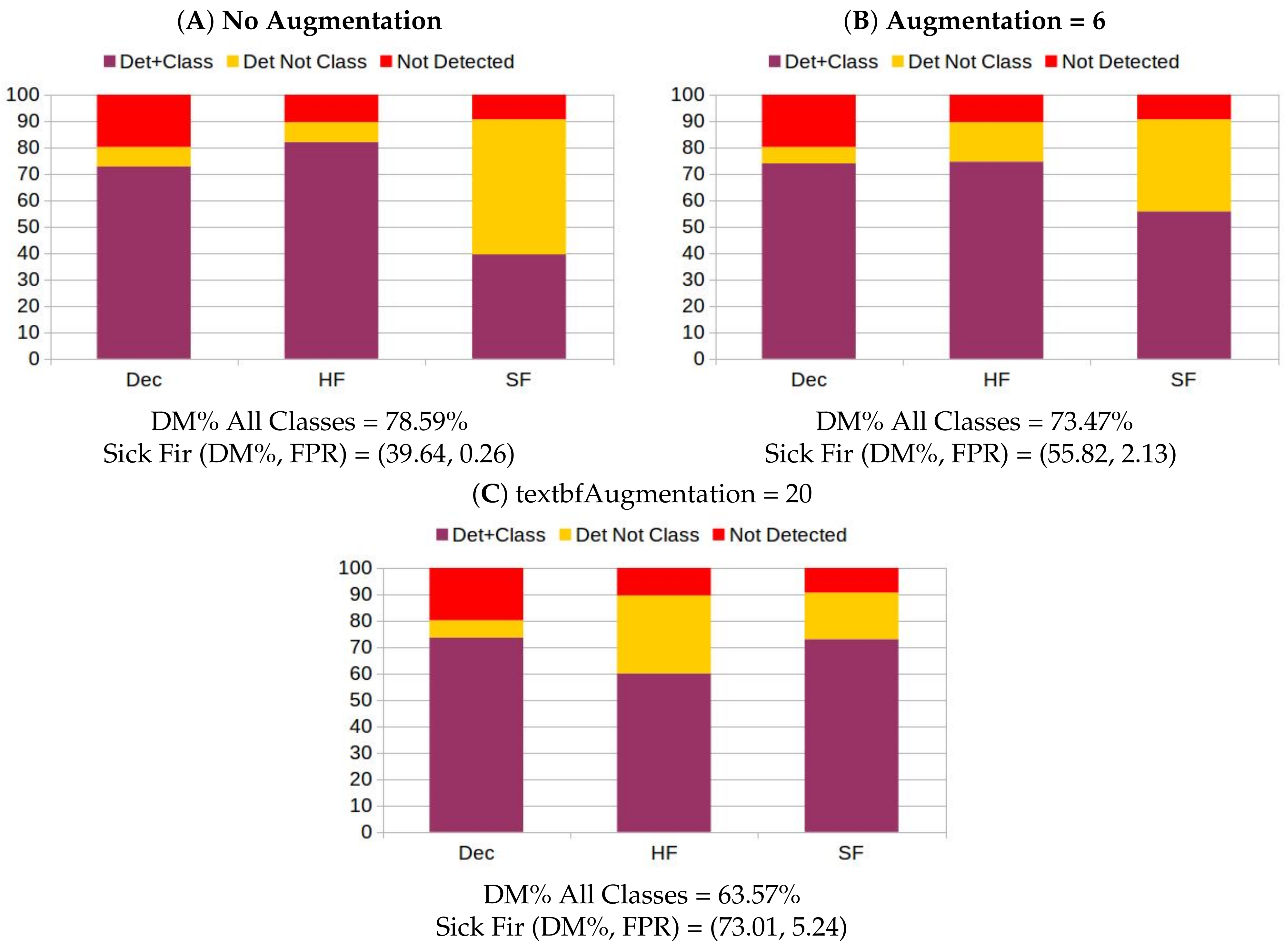
Concerning data augmentation, for each of the scenarios considered before, we used the learning rate value that had showed the best results in the classification experiment using ground truth points. Additionally, in this experiment the practical use of the resulting classifier networks were considered and three “use cases” were summarised (Figure 8). First in part (A) of the figure, data augmentation was not used in order to maximize the total classification accuracy of the network. Second part (B), a small amount of data augmentation was used to increase the specificity of the sick fir class while retaining most of the networks overall classification accuracy. Finally, part C contained information of a classifier that relied heavily on data augmentation to provide the maximum sensitivity for the sick fir class at the cost of decreasing the overall number of correctly classified trees among all classes.
Our algorithms can be used to gain valuable insight both into the tree type distribution of the studied forests as well as the health status of the fir trees. On the first case (A), the combination of our algorithms without using data augmentation provides us with a description of the location of trees and tree type distribution that automatically places and identifies correctly 78.59% of the trees. This shows that the analysis of drone-acquired images using computer vision and DL techniques presents opportunities for forest research in a much larger scale than what was previously possible.
Although there was 85.07% of trees successfully detected (80.16% for deciduous, 89.6% for healthy fir and 90.65% for sick fir), the first case had the problem that the specificity of the sick fir class was low with 39.64%, while 72.80% of deciduous trees and 82.07% of healthy fir trees were detected and classified correctly. The low detection + classification result for sick trees was mainly due to miss-classification. However, this first case has the problem that the specificity of the sick fir class is low. The value of approximately 40% specificity is coherent with the observed classification of ground truth treetops where the relatively low number of sick fir trees resulted in low sensitivity for this class. Using data augmentation in the classification part of the algorithm resulted in improved sensitivity for this class. This is achieved at the cost of decreased accuracy for the healthy fir and deciduous classes.
The second case showed that using a moderate amount of data augmentation (6 synthetic images are created for each real image in the training set of each fold of the leave-one-out strategy) can increase the number of sick fir trees detected (up to 55.82%) at the cost of about a 5% loss in the percentage of trees correctly detected and classified (from 78.59% to 74.47%). This loss is better put into context by looking at the decrease in the number of False Positives produced for every positive detection. In this case, in order to detect approximately half of the sick fir trees, 2.13 False Positive predictions were detected for each True Positive. Taking into consideration, the infrequent occurrence of the sick fir class, the overall accuracy of the system is still high. Finally, a wider use of data augmentation (with 20 sick fir images created out of each original one) resulted in a percentage of correctly detected and classified sick fir treetops that rose to 73.01% (which stands at 80.54% of the 90.65% of detected sick fir trees correctly classified). The cost of this increase is a larger FPR for sick fir (raising to 5.24 from 2.21) that resulted in a higher impact of the total performance of the system (with the percentage of deciduous trees correctly detected and classified) slightly decreasing to 73.61% and that of healthy fir trees registering a sharp decrease down to 60.05%.

4. Discussion

4.1. Data Challenges

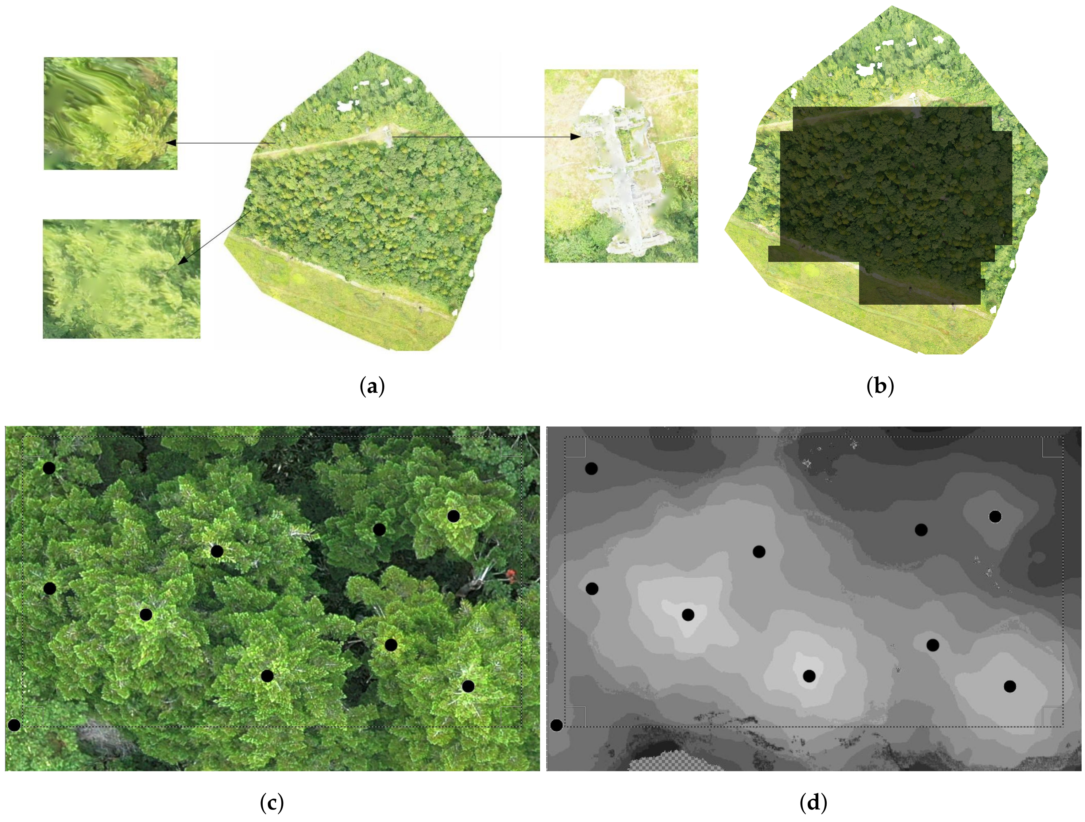
The research area is a natural mountainous forest. That presents high heterogeneity in terms of tree height, age and the tree type distribution within each of the study sites. While the use of UAV allow the collection of high-resolution data in wide extensions of this difficult-to-access area, the data still presents some challenges. For example, after using the UAV-acquired images to build orthomosaics and DSM, the orthomosaics contained information extraneous to our purposes such as buildings, power lines or power towers. Additionally, and due to the flight pattern followed for data acquisition, the border sections of the orthomosaics contained heavy image distortions. Figure 9a presents examples of these two issues. In order to partially address these issues, for each orthomosaic we selected a Region Of Interest (ROI) in its central part and focused our computations within that region (Figure 9b ). Additionally, the mountainous terrain resulted in the height values encoded in the DSM including in each pixel both the altitude of any trees present along with the terrain elevation. This severely hampered the automatic detection of treetops as the slope create the same elevation values of treetop downhill and the ground uphill (Figure 4c). This problem was dealt by normalizing the slope with the Fusion/LDV software [21] and having the ground removed by the software Global Mapper [42] (see Section 2.2 for details). Furthermore, some treetops were not distinguishable even in the nDSM. This happened particularly when larger, taller trees where very close to smaller trees with lower treetops. Figure 9c,d presents an example of this. Even though 10 treetops are visible in the orthomosaic, only 4 clear distinct regions are visible in the nDSM. Although those treetops were not visible on the nDSM, they were still marked in the annotation step for the validation, but there is a high chance that they would not be found by any detection algorithm that uses elevation data to detect treetops (such as the one presented in this work).
The use of the pre-processing step described in Section 2.2 allowed us to focus the detection and classification efforts in the parts of the orthomosaics and DSMs that correspond to tree canopies. Furthermore our treetop detection algorithm is based on exploring pixel altitude values starting with higher values (expected to belong to treetop tips). This makes it necessary to mitigate the distorting effect of the terrain in the elevation values by using the nDSM, which resulted in the loss of 2% of the treetops (Table 1). Most of the lost treetops were located in parts of the orthomosaics that were out of the ROI (Figure 6) described in Section 4.1. The number of trees left after the pre-processing step (5364 trees, with 169 sick fir trees) was larger than the number of trees considered in other studies (336 in the testing set in [9] or 931 tree samples in the testing set in [20] for example).
The 85.70% matching percentage obtained by the algorithm represents a clear improvement compared to existing methods (71.50% for the second-best method studied [11]). Most treetop detection mistakes occurred when deciduous trees were detected (80.16% matching percentage) while the fir classes presented even better performances (89.6% for healthy fir and 90.65% for sick fir). The counting criterion (cnt) results showed that the method used tends to overestimate the number of existing trees (by 9.67% on average) (Table 2), while other methods obtained better results in relation to the counting criterion for some sites. For example, for nDSM 1 our method obtained 89.61% matching with an overestimation of 9.87% of the number of treetops (yielding, thus, 81.56% of matched points among those predicted). On the other hand, the implementation of the Dawkins method used in [9] obtained 70.54% matching with 2.18% of treetop underestimation (representing a 72% of success). In comparison, our method found more ground truth points and made stronger predictions which can be explained by the fact that the data used in [9] was slightly different. While the tree species and the tree health problems studied are the same, the boreal conditions in Siberia decreased the biodiversity (where the forest studied in [9] is located) so only fir trees are present which allows a clear visualization of individual trees. In this respect, nDSM 9, corresponding to the top site and with poor presence of deciduous trees may be more similar to the data in [9].
The higher performance of our algorithm over the other algorithms considered is also supported by the average Euclidean distance metric. This method obtained a low value of just over 50 pixels (slightly under one meter) from any predicted point to the closest ground truth point. This value becomes as low as 27.42 pixels when other matched points were considered. The merits of these results are highlighted by taking into account the multiple data challenges previously mentioned. The effects of these particular conditions can be appraised by comparing the results of the GMax ( m % : 71.42 , c n t : 10.22 ) and FCM ( m % : 71.50 , c n t : 10.24 ) methods with the data of our study to the ones they obtained in [11] ( m % : 90 , c n t : 9 ). The decrease in performance is due to the differences in data as well as the more strict matching conditions expressed by the ϵ parameter (3 m in [11] compared to 2–2.5 in our study). We consider that these strict conditions coupled with the larger amount of data compared to other papers in the research area showcase the importance of the results achieved. The difference with previous studies also showed how this part of the algorithmic process is the most challenging and that further progress is likely possible.
The performance of five existing DL networks were studied (AlexNet, Squeezenet, Vgg, ResNet and DenseNet) to classify the patches around treetops. Ground truth treetops were used to evaluate the performance of this part of our algorithmic process independently. Initial results using all data from all orthomosaics showed that all networks were able to obtain low error rates, especially Vgg (with the best value of ER = 0.03357%); ResNet and DenseNet performed well (Figure 7). However, the sick fir class was frequently missed and the low error rates reflected its low occurrence rate (Table 3). While the numbers showed that the studied networks performed well, concerns towards their practical use arose. In order to address this issue as well as overfitting, a site-wise leave-one-out strategy was used to make sure that the training and testing sets never contained images from the same trees (even if taken in different flights and with different lighting conditions). Results showed that data augmentation succeeded in increasing the importance of the sick fir class during the training process and, thus, increase the sensitivity values obtained (Table 4). This was coupled with minor decreases in specificity and accuracy for the sick fir class (0.9810,0.9809) for the Resnet network when using 10 augmented images for each real sick fir image. The decrease in specificity produced that some images that did not contain sick fir trees were wrongly predicted as such (False Positive detections). This resulted in slightly decreased accuracy values for the other classes (0.9601 accuracy of healthy fir). These results, even those with slightly lower accuracy, were in the higher band of the results obtained in previous studies (91.95–98.97% accuracy to classify sick fir in [9], 94.01–97% in [12] to distinguish between deciduous and evergreen trees or 73.25% accuracy for multi-species classification in [20]).
Finally, the performance of all the algorithms introduced in the paper was studied when applied to solve the real-life problem of classifying tree health and types classes found in forest sites. After adapting the training sets to account for the fact that the automatically detected treetops were not perfectly centered on the tree trunks, we aimed at assessing how many trees in the three categories were correctly detected and classified. After exploring different data augmentation scenarios three different use cases for our algorithms were presented. In the first case, working with the original data without data augmentation we were able to correctly detect and classify over 78% of the trees, giving a reliable description of the tree type distribution of the forest with percentages of correctly detected and classified trees of 72.80% and 82.07% for deciduous and healthy fir, respectively. The biggest downside of this case was the relatively low success rate in the classification of sick fir trees. Although 90.65% of sick fir trees where detected over all sites, only 39.64% of them were correctly classified with most of them misclassified as healthy. These results were in line with the tendency observed in the experiment where ground truth points had been used for classification, the low number of sick fir trees resulted in this class being mostly ignored in the training process and in a low specificity result. However, even in this situation, the information resulting from our algorithm was of practical use. A detailed analysis for each site showed that the algorithm found 3/20 sick fir trees in site 1, 13/49 in site 2, 7/20 in site 3 and 44/80 in site 4. The results missed a small cluster containing 4 trees in the orthomosaic 1 but otherwise found sick trees in all other affected regions (including one in a region containing only three sick trees in orthomosaic 3). The algorithm tended to underestimate the extent of the regions affected by classifying the less affected trees as healthy but correctly identified the affected regions. As mentioned before, the definition of “sick” fir is slightly open to interpretation, especially, when trees presenting slight defoliation (Figure 2b) are considered healthy while others with slightly more defoliation, sometimes obscured by top branches with green leaves (Figure 2c) are considered sick. Because of this, in practice any cluster of sick trees detected using the algorithm would need to be confirmed by expert analysis of the drone images and, if at all possible, with observations on the ground. Nevertheless, the results presented here show that this version of the algorithms can be used as an automatic early warning tool to detect even minor bark beetle outbreaks.
In the other two cases presented, data augmentation was used to increase the importance of the sick fir class during training in order to increase its specificity. This was achieved at the cost of producing a number of False Positive detections, mostly by classifying healthy fir trees as sick. In the “balanced” case (augm 6) we could detect 55.82% of the sick fir trees producing 2.13 extra False Positive detections for each correct one (FPR 2.23) and in the case where we focused in the detection of sick fir trees (augm 20) we detected 73.01% of them at the cost of an FPR of 5.24. Both of these approaches correctly detected and classified trees in all outbreak regions at the price of overestimating their extension. The somewhat difficult distinction between sick and healthy fir played a reverse role to the first use case with most of the False Positive sick fir detections being found in areas close to outbreaks but marked as healthy. Although this may provide users with wrong information and exaggerating the extent of the outbreaks it can also be seen as a way to point out possible areas of outbreak development.

5. Conclusions

The study presented algorithms for the automatic detection and classification of fir trees (healthy and sick in terms of a bark beetle infestation) as well as deciduous trees. The detection of individual treetops was found to be a key part of the process that had not been studied in enough detail so far. Our results, including the comparison of three state of the art methods showed that the algorithm for treetop detection introduced in the current work was able to detect 85.70% of existing trees, outperforming existing methods in experiments that were challenging both in terms of the data used and the quality criteria considered. We then moved on to show how, as seen in other application domains, DL networks can successfully learn to classify the classes present in our problem (obtaining over 98% accuracy on average over the three classes). However, in this case a careful use of data augmentation was needed to obtain results that not only presented good classification metrics but were also meaningful in practice. We have also presented what is, to the best of our knowledge, a detailed study of the performance of all the algorithms presented when used together, paying special attention to the sources of error and to their practical implications. In terms of the detection of sick fir trees, the main goal of our study, we showed how just under 10% of the points were not detected and how the amount of remaining points correctly classified depended on how data augmentation was used. In one use case, our algorithms were able to detect and classify correctly 78% of the trees in all species. This algorithm was also able to detect all but one of the existing outbreak clusters (composed of 4 sick trees) where it detected only about 40% of the existing sick trees. This percentage was increased to 73.01% at the price of producing a large number of false positive detections. Consequently, we have shown how computer vision and DL networks when used to process UAV-acquired images, already provide a valuable tool for the automatic detection and monitoring of sick fir trees with tangible benefits in terms of study time, human resources needed and extent of land area required for study.
Regarding future research directions, the treetop detection algorithm could be improved by considering the detection of treetops of each separate species individually since a 10% discrepancy in the percentage of successfully detected trees was observed between fir and deciduous trees. Regarding the classification algorithm, collecting datasets with a larger number of sick tree examples would reduce the need to use data augmentation and, with it, the number of false positive detections. This would also open the possibility to DL networks with a larger number of layers and optimizable parameters.

Author Contributions

H.T.N., Y.D., M.L.L.C., K.M., S.K. and H.S. conceived the conceptualization and methodology, supported the writing—review and editing. Y.D., H.T.N. and K.M. developed the software, performed the validation, investigation. H.T.N., Y.D., M.L.L.C. writing—original draft preparation. H.T.N. and Y.D. carried out formal analysis. H.T.N. and M.L.L.C. administrated the data. H.T.N. and Y.D. performed the visualization. M.L.L.C. and Y.D. supervised the project and provided resources. M.L.L.C.and Y.D. directed the project administration. All authors have read and agreed to the published version of the manuscript.

Funding

This research received no lexternal funding.

Acknowledgments

The authors of this paper want to acknowledge the authors of [9] for making their source code publicly available. We also want to thank Hiroaki Funatsu from the Tohoku Regional Forest University for his support facilitating our fieldwork in Zao.

Conflicts of Interest

The authors declare no conflict of interest.

References

  1. Jactel, H.; Koricheva, J.; Castagneyrol, B. Responses of forest insect pests to climate change: Not so simple. Curr. Opin. Insect Sci. 2019, 35, 103–108. [Google Scholar] [CrossRef] [PubMed]
  2. Agne, M.C.; Beedlow, P.A.; Shaw, D.C.; Woodruff, D.R.; Lee, E.H.; Cline, S.P.; Comeleo, R.L. Interactions of predominant insects and diseases with climate change in Douglas-fir forests of western Oregon and Washington, USA. For. Ecol. Manag. 2018, 409, 317–332. [Google Scholar] [CrossRef] [PubMed]
  3. Przepióra, F.; Loch, J.; Ciach, M. Bark beetle infestation spots as biodiversity hotspots: Canopy gaps resulting from insect outbreaks enhance the species richness, diversity and abundance of birds breeding in coniferous forests. For. Ecol. Manag. 2020, 473, 118280. [Google Scholar] [CrossRef]
  4. Krokene, P.; Solheim, H. Pathogenicity of four blue-stain fungi associated with aggressive and nonaggressive bark beetles. Phytopathology 1998, 88, 39–44. [Google Scholar] [CrossRef] [Green Version]
  5. Rice, A.V.; Thormann, M.N.; Langor, D.W. Mountain pine beetle associated blue-stain fungi cause lesions on jack pine, lodgepole pine, and lodgepole× jack pine hybrids in Alberta. Botany 2007, 85, 307–315. [Google Scholar] [CrossRef]
  6. Six, D.; Paine, T. Effects of mycangial fungi and host tree species on progeny survival and emergence of Dendroctonus ponderosae (Coleoptera: Scolytidae). Environ. Entomol. 1998, 27, 1393–1401. [Google Scholar] [CrossRef]
  7. Näsi, R.; Honkavaara, E.; Lyytikäinen-Saarenmaa, P.; Blomqvist, M.; Litkey, P.; Hakala, T.; Viljanen, N.; Kantola, T.; Tanhuanpää, T.; Holopainen, M. Using UAV-based photogrammetry and hyperspectral imaging for mapping bark beetle damage at tree-level. Remote Sens. 2015, 7, 15467–15493. [Google Scholar] [CrossRef] [Green Version]
  8. Smigaj, M.; Gaulton, R.; Barr, S.; Suárez, J. UAV-borne thermal imaging for forest health monitoring: Detection of disease-induced canopy temperature increase. Int. Arch. Photogramm. Remote. Sens. Spat. Inf. Sci. 2015, 40, 349. [Google Scholar] [CrossRef] [Green Version]
  9. Safonova, A.; Tabik, S.; Alcaraz-Segura, D.; Rubtsov, A.; Maglinets, Y.; Herrera, F. Detection of fir trees (Abies sibirica) damaged by the bark beetle in unmanned aerial vehicle images with deep learning. Remote Sens. 2019, 11, 643. [Google Scholar] [CrossRef] [Green Version]
  10. Pulido, D.; Salas, J.; Rös, M.; Puettmann, K.; Karaman, S. Assessment of tree detection methods in multispectral aerial images. Remote Sens. 2020, 12, 2379. [Google Scholar] [CrossRef]
  11. Diez, Y.; Kentsch, S.; Lopez-Caceres, M.L.; Nguyen, H.T.; Serrano, D.; Roue, F. (Eds.) Comparison of Algorithms for Tree-top Detection in Drone Image Mosaics of Japanese Mixed Forests. Proceeding of the 9th International Conference on Pattern Recognition Applications and Methods, INSTICC, Valletta, Malta, 22–24 February 2020; SciTePress: Setúbal, Portugal, 2020. [Google Scholar]
  12. Kentsch, S.; Lopez Caceres, M.L.; Serrano, D.; Roure, F.; Diez, Y. Computer Vision and Deep Learning Techniques for the Analysis of Drone-Acquired Forest Images, a Transfer Learning Study. Remote Sens. 2020, 12, 1287. [Google Scholar] [CrossRef] [Green Version]
  13. Krisanski, S.; Taskhiri, M.S.; Turner, P. Enhancing methods for under-canopy unmanned aircraft system based photogrammetry in complex forests for tree diameter measurement. Remote Sens. 2020, 12, 1652. [Google Scholar] [CrossRef]
  14. Brovkina, O.; Cienciala, E.; Surovỳ, P.; Janata, P. Unmanned aerial vehicles (UAV) for assessment of qualitative classification of Norway spruce in temperate forest stands. Geo-Spat. Inf. Sci. 2018, 21, 12–20. [Google Scholar] [CrossRef] [Green Version]
  15. Michez, A.; Piégay, H.; Lisein, J.; Claessens, H.; Lejeune, P. Classification of riparian forest species and health condition using multi-temporal and hyperspatial imagery from unmanned aerial system. Environ. Monit. Assess. 2016, 188, 146. [Google Scholar] [CrossRef] [PubMed] [Green Version]
  16. Vastaranta, M.; Holopainen, M.; Yu, X.; Hyyppä, J.; Mäkinen, A.; Rasinmäki, J.; Melkas, T.; Kaartinen, H.; Hyyppä, H. Effects of individual tree detection error sources on forest management planning calculations. Remote Sens. 2011, 3, 1614–1626. [Google Scholar] [CrossRef] [Green Version]
  17. Bennett, G.; Hardy, A.; Bunting, P.; Morgan, P.; Fricker, A. A transferable and effective method for monitoring continuous cover forestry at the individual tree level using UAVs. Remote Sens. 2020, 12, 2115. [Google Scholar] [CrossRef]
  18. Dash, J.P.; Watt, M.S.; Pearse, G.D.; Heaphy, M.; Dungey, H.S. Assessing very high resolution UAV imagery for monitoring forest health during a simulated disease outbreak. ISPRS J. Photogramm. Remote Sens. 2017, 131, 1–14. [Google Scholar] [CrossRef]
  19. Sylvain, J.D.; Drolet, G.; Brown, N. Mapping dead forest cover using a deep convolutional neural network and digital aerial photography. ISPRS J. Photogramm. Remote. Sens. 2019, 156, 14–26. [Google Scholar] [CrossRef]
  20. Sun, Y.; Huang, J.; Ao, Z.; Lao, D.; Xin, Q. Deep Learning Approaches for the Mapping of Tree Species Diversity in a Tropical Wetland Using Airborne LiDAR and High-Spatial-Resolution Remote Sensing Images. Forests 2019, 10, 1047. [Google Scholar] [CrossRef] [Green Version]
  21. McGaughey, R.J. FUSION/LDV: Software for LIDAR Data Analysis and Visualization; US Department of Agriculture, Forest Service, Pacific Northwest Research Station: Seattle, WA, USA, 2009; Volume 123. [Google Scholar]
  22. Pleșoianu, A.I.; Stupariu, M.S.; Șandric, I.; Pătru-Stupariu, I.; Drăguț, L. Individual Tree-Crown Detection and Species Classification in Very High-Resolution Remote Sensing Imagery Using a Deep Learning Ensemble Model. Remote Sens. 2020, 12, 2426. [Google Scholar] [CrossRef]
  23. Dupret, G.; Koda, M. Bootstrap re-sampling for unbalanced data in supervised learning. Eur. J. Oper. Res. 2001, 134, 141–156. [Google Scholar] [CrossRef]
  24. Krizhevsky, A.; Sutskever, I.; Hinton, G.E. ImageNet Classification with Deep Convolutional Neural Networks. In Proceedings of the 25th International Conference on Neural Information Processing Systems, Lake Tahoe, NV, USA, 3–6 December 2012; Volume 1, pp. 1097–1105. [Google Scholar]
  25. Iandola, F.N.; Moskewicz, M.W.; Ashraf, K.; Han, S.; Dally, W.J.; Keutzer, K. SqueezeNet: AlexNet-level accuracy with 50× fewer parameters and <1MB model size. arXiv 2016, arXiv:1602.07360. [Google Scholar]
  26. Simonyan, K.; Zisserman, A. Very Deep Convolutional Networks for Large-Scale Image Recognition. In Proceedings of the International Conference on Learning Representations, San Diego, CA, USA, 7–9 May 2015. [Google Scholar]
  27. He, K.; Zhang, X.; Ren, S.; Sun, J. Deep Residual Learning for Image Recognition. arXiv 2015, arXiv:1512.03385. [Google Scholar]
  28. Huang, G.; Liu, Z.; Weinberger, K.Q. Densely Connected Convolutional Networks. In Proceedings of the 2017 IEEE Conference on Computer Vision and Pattern Recognition (CVPR), Honolulu, HI, USA, 21–26 July 2016; pp. 2261–2269. [Google Scholar]
  29. Cabezas, M.; Kentsch, S.; Tomhave, L.; Gross, J.; Caceres, M.L.L.; Diez, Y. Detection of Invasive Species in Wetlands: Practical DL with Heavily Imbalanced Data. Remote Sens. 2020, 12, 3431. [Google Scholar] [CrossRef]
  30. Shiferaw, H.; Bewket, W.; Eckert, S. Performances of machine learning algorithms for mapping fractional cover of an invasive plant species in a dryland ecosystem. Ecol. Evol. 2019, 9, 2562–2574. [Google Scholar] [CrossRef] [PubMed] [Green Version]
  31. Deng, L.; Yu, R. Pest Recognition System Based on Bio-Inspired Filtering and LCP Features. In Proceedings of the 2015 12th International Computer Conference on Wavelet Active Media Technology and Information Processing (ICCWAMTIP), Chengdu, China, 18–20 December 2015; pp. 202–204. [Google Scholar] [CrossRef]
  32. Zhao, X.; Zhang, J.; Tian, J.; Zhuo, L.; Zhang, J. Residual Dense Network Based on Channel-Spatial Attention for the Scene Classification of a High-Resolution Remote Sensing Image. Remote Sens. 2020, 12, 1887. [Google Scholar] [CrossRef]
  33. Masarczyk, W.; Głomb, P.; Grabowski, B.; Ostaszewski, M. Effective Training of Deep Convolutional Neural Networks for Hyperspectral Image Classification through Artificial Labeling. Remote Sens. 2020, 12, 2653. [Google Scholar] [CrossRef]
  34. Onishi, M.; Ise, T. Automatic classification of trees using a UAV onboard camera and deep learning. arXiv 2018, arXiv:1804.10390. [Google Scholar]
  35. Natesan, S.; Armenakis, C.; Vepakomma, U. Resnet-Based Tree Species Classification Using Uav Images. ISPRS Int. Arch. Photogramm. Remote. Sens. Spat. Inf. Sci. 2019, 42, 475–481. [Google Scholar] [CrossRef] [Green Version]
  36. 3.10 Q QGIS Geographic Information System. Open Source Geospatial Foundation Project. Available online: http://qgis.org/ (accessed on 7 December 2019).
  37. Schomaker, M. Crown-Condition Classification: A Guide to Data Collection and Analysis; US Department of Agriculture, Forest Service, Southern Research Station: Asheville, NC, USA, 2007; Volume 102. [Google Scholar]
  38. Agisoft, L. Agisoft Metashape, Professional Edition, Version 1.5.5. Available online: http://agisoft.com/ (accessed on 19 March 2020).
  39. Team, T.G. GNU Image Manipulation Program. Available online: http://gimp.org (accessed on 19 August 2019).
  40. Van Rossum, G.; Drake, F.L., Jr. Python Tutorial; Centrum voor Wiskunde en Informatica: Amsterdam, The Netherlands, 1995. [Google Scholar]
  41. Kraus, K.; Pfeifer, N. Determination of terrain models in wooded areas with airborne laser scanner data. ISPRS J. Photogramm. Remote. Sens. 1998, 53, 193–203. [Google Scholar] [CrossRef]
  42. Geographics, B.M. Global Mapper Version 21.1. Available online: https://www.bluemarblegeo.com/ (accessed on 24 June 2020).
  43. Howard, J.; Thomas, R.; Gugger, S. Fastai. Available online: https://github.com/fastai/fastai (accessed on 18 April 2020).
  44. Jung, A.B.; Wada, K.; Crall, J.; Tanaka, S. Imgaug. 2020. Available online: https://github.com/aleju/imgaug (accessed on 1 July 2020).
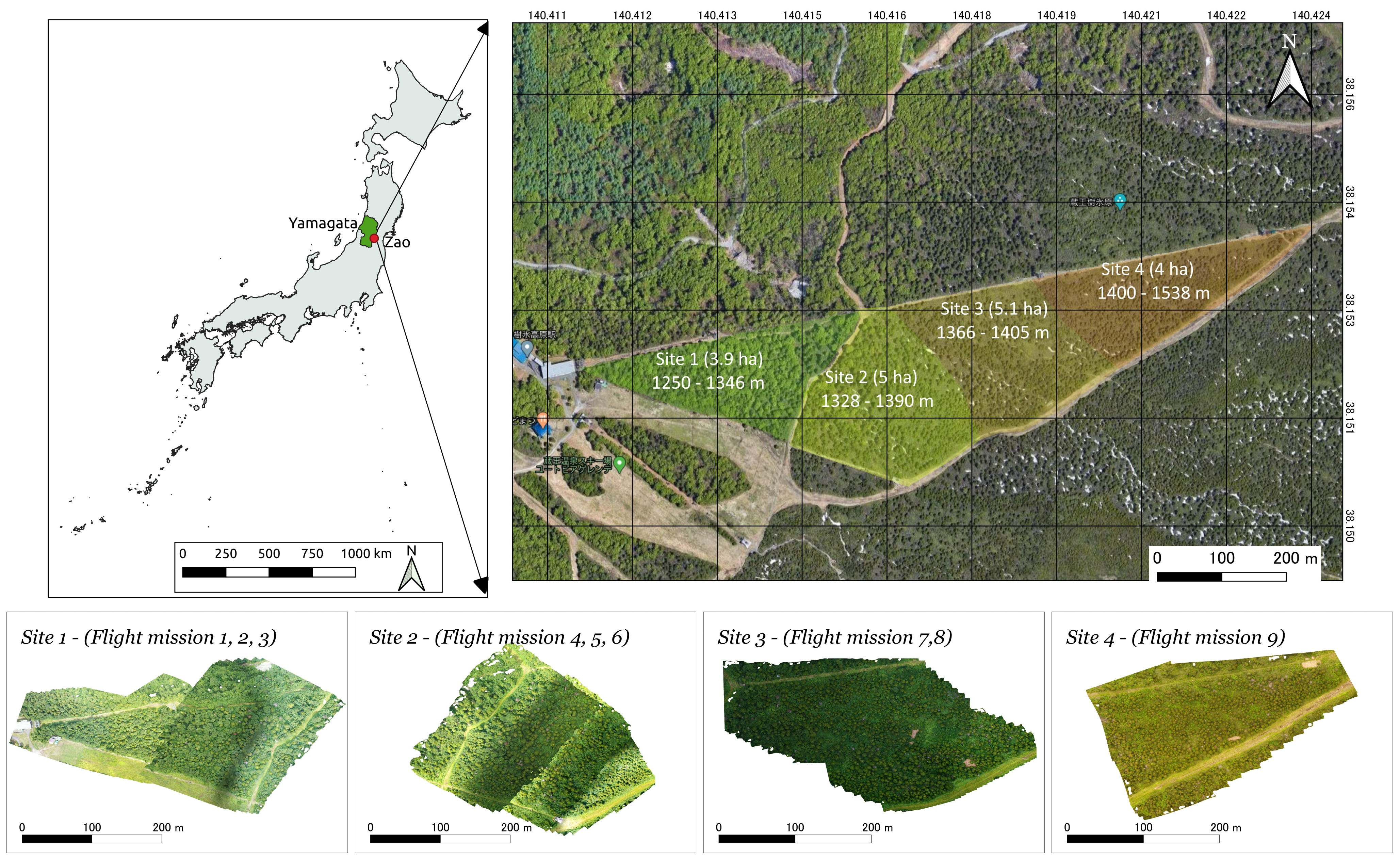
Figure 1. The four study sites are located in Zao Mountain, Yamagata prefecture, Japan. A gradual increase in elevation from site 1 to site 4 together with the increasing number of fir trees infested by bark beetles, followed by the decrease of mixing rate with deciduous species (background map from Google Hybrid [36]).
Remotesensing 13 00260 g001
Figure 2. (a) healthy fir (HF) fully covered by green leaves; (b) healthy fir (HF) with minimal defoliation; (c) sick fir (SF) with some leafless branches at the bottom; (d) sick fir (SF) with majority of leafless branches; (eg) broadleaf (BL) in site 1 and 2.
Remotesensing 13 00260 g002
Figure 3. Algorithm pipeline used in this study. Blue, processed data in different formats. White with dash green border, external software used. Dark Green, algorithms developed as part of our study. Red, results of algorithms. Orange, validation steps.
Remotesensing 13 00260 g003
Figure 4. (a) DSM and (b) nDSM, the lighter (white) pixels represent high elevations and darker pixels represent low elevations, the black pixel on nDSM represents no value ot the excluded ground and lower vegetation area; (c) the elevation profile of a random area on the DSM at an altitude of 1320 m as a treetop downhill is at the same altitude of the ground uphill (red circles).
Remotesensing 13 00260 g004
Figure 6. (a,b) annotated treetops on small trees were in DSM (left) but do not appear on the nDSM (right). The floor regions in the nDSM have been left transparent so the part of the orthomosaic considered as ′floor″ is clearly visible. The treetops missed are, thus, those painted over RGB (not grayscale) areas.
Remotesensing 13 00260 g006
Figure 7. Error Rate Results for tree health classification for all learning rates and DL architectures.
Remotesensing 13 00260 g007
Figure 8. Detection and classification of trees according to species and health categories. Three graphs are presented according to three use cases of our algorithm (A) No Data Augmentation. Focus on species separation, (B) Data Augmentation = 6. Balanced Use case. (C) Data Augmentation = 20. Focus on Sick Fir detection. The graphs include: Percentage of treetops missed in the detection step (top), Percentage of treetops detected but not classified correctly (middle) and Percentage of treetops detected and classified correctly (down). Each graph contains information on the three classes studied: Healthy Fir (HF), Sick Fir (SF) and Deciduous (BL). Finally, the percentage of trees correctly detected and classified over the three classes is provided as “DM% All Classes”. The percentage of correctly detected and classified Sick Fir trees as well as the ratio of False Positive predictions (FPR) for the same category are also provided. All the percentages reported correspond to the total number of trees present as expressed by the ground truth.
Remotesensing 13 00260 g008
Figure 9. (a) artifact and distortion at the edge present in the orthomosaic; (b) ROI was applied to eliminate the artifacts and the disorted edge; (c) 10 Trees present in orthomosaic but (d) only 4 trees have clear distinct regions in nDSM.
Remotesensing 13 00260 g009
Table 1. Percentage of annotated treetop lost when using nDSM instead of DSM.
nDSM123456789Average
% treetop lost1.121.570.176.903.082.250.001.003.202.14
Table 2. Tree crown detection method performance. Results of the matching percentage (m%) and counting measure (cnt) are presented for each nDSM and the total average. Positive values for the cnt criterion indicate underestimation of the number of trees present while negative values indicate overestimation. For this criterion the average of absolute values was computed. This table show the result using our data with previously reported algorithm.
nDSM12345
Methodm%cntm%cntm%cntm%cntm%cnt
OUR Approach89.619.8780.1414.5190.475.6782.9714.1585.618.73
Dawkins  [9]70.542.1854.6113.7973.416.9259.7916.3251.1219.35
GM  [11]71.17−9.2160.75−11.1178.35−9.8270.09−8.1269.81−9.76
FCM [11]66.22−9.7461.68−12.3773.56−12.2573.21−7.2569.49−9.05
nDSM6789AVERAGE
Methodm%cntm%cntm%cntm%cntm%cnt
Our Approach85.718.3780.527.74809.2496.298.7885.709.67
Dawkins [9]50.0622.4370.691.2771.368.7992.613.3166.0210.48
GM  [11]68.85−14.8263.27−9.4472.82−12.2787.67−7.4171.4210.22
FCM  [11]72.2−10.1864.71−17.8772.3−7.7690.14−5.7171.5010.24
Table 3. Sensitivity, Specificity and Accuracy values for the classification of treetop patches according to health.
SensitivitySpecificityAccuracy
Deciduous0.9820.9990.995
Healthy Fir0.9950.9260.976
Sick Fir0.5130.9960.980
Table 4. Results for the sick fir class for three DL networks and five data augmentation scenarios. Values for the LR obtaining best specificity are shown for all augmentation scenarios. augm “n” stands for a data augmentation scenario where “n” images are created for each existing sick fir image.
DenseNetResNetVGG
SensSpecAccSensSpecAccSensSpec
no augm0.41090.99590.97710.44220.99120.97380.40010.99310.9761
augm 20.67720.99480.97630.71990.99410.97820.65760.99210.9752
aumg 60.93820.98750.97960.94070.98630.97880.93910.98770.9787
augm 100.98060.98390.98340.97940.98100.98090.97920.9810.9794
augm 200.99360.97690.98360.99720.98220.98800.98680.98050.9791
Publisher’s Note: MDPI stays neutral with regard to jurisdictional claims in published maps and institutional affiliations.