Abstract
Benchmarking deep learning algorithms before deploying them in hardware-constrained execution environments, such as imaging satellites, is pivotal in real-life applications. Although a thorough and consistent benchmarking procedure can allow us to estimate the expected operational abilities of the underlying deep model, this topic remains under-researched. This paper tackles this issue and presents an end-to-end benchmarking approach for quantifying the abilities of deep learning algorithms in virtually any kind of on-board space applications. The experimental validation, performed over several state-of-the-art deep models and benchmark datasets, showed that different deep learning techniques may be effectively benchmarked using the standardized approach, which delivers quantifiable performance measures and is highly configurable. We believe that such benchmarking is crucial in delivering ready-to-use on-board artificial intelligence in emerging space applications and should become a standard tool in the deployment chain.
1. Introduction
Computing hardware platforms are mainly used in space missions for data transfer that involves sending raw data (e.g., imagery and video streams) to ground stations, while data processing is done in centralized servers on Earth. Large data transfers cause network bottlenecks and increases latency, thus increasing the system response time. For safety-critical industry applications, such as aerospace and defense, latency is a major concern; hence, optimizing it is an important research topic [1,2,3,4].
AI-dedicated computing hardware platforms have become increasingly important in a variety of space applications as they provide a set of features to allow for efficient computation tasks. Thanks to them, deep learning inference can be effectively executed very close to the data sources (e.g., imaging sensors) at the edge device. This may improve the spacecraft autonomy, mitigate a costly requirement of transmitting large volumes of data to a remote processing site, accelerate decision-making, and increase reliability in communication-denied environments (i.e., in space). Nevertheless, each piece of computing hardware comes with inherent features and constraints that enable or disrupt performance depending on the deep model and targeted applications. In addition, deep learning models must be adopted to make “optimal” use of the underlying hardware infrastructure.
This paper presents the approach for benchmarking state-of-the-art AI models for a range of space applications focused on computer vision tasks, such as image classification or object detection. Such applications in which image and video data are processed reach beyond the specific tasks tackled in this work and could include imaging support for autonomous space vehicle docking, decision support for autonomous probes or landers, autonomous robotic systems, satellite star trackers, Earth observation targeting decision support, and many more [5]. Although an unprecedented level of success of deep learning in virtually all fields of science and industry has been witnessed, thorough verification and validation of deep models before deploying them in the wild remain under-explored in the literature. This issue is tackled in this work; in Section 1.2, the contributions are discussed in more detail. Benchmarking AI models before final deployment can lead to a better understanding of available resources and a more robust delivery of deep learning solutions for on-orbit devices.
1.1. Related Work and Motivation
Benchmarking deep learning algorithms for on-board space applications is getting research attention due to a number of emerging missions, e.g., in Earth observation, where such techniques are to be deployed on-board the spacecraft. Moreover, there exists a set of well-established tools for developing, verifying, and validating deep learning on Earth, selecting an appropriate toolchain and utilizing it to benchmark on-board deep learning remains an open question in the literature. In recent years, TensorFlow Lite has been a popular choice for developing embedded AI applications. Agostini et al. proposes a framework for designing software and hardware solutions with TensorFlow Lite and the SystemC event-driven simulator [6]. Contrary to the work presented here, it features a broader look at embedded AI devices with different technologies, while our efforts focus on specific neural network models and hardware devices that will be exploited in orbit on-board our Intuition-1 mission, being a 6U-class satellite with a data processing unit, referred to as the Leopard Deep Learning Processing Unit (DPU), enabling on-board data analysis acquired via a hyperspectral imagery.
MLPerf is a benchmarking system that creates a common denominator for comparing software and hardware solutions for AI inference [7]. It allows us to introduce a software suite of on-orbit specific benchmarks in order to get “closer” to deploying AI models in space. However, MLPerf is not implemented in a strict sense, as the main goal is not to directly compare the hardware performance. Instead, some well-established benchmarking solutions from the industry-standard MLPerf are utilized, and they are applied to the investigated use cases. The objective is to perform tests that investigate crucial aspects of on-orbit AI devices while fully utilizing their capabilities. The publication by Boutros et al. can be used as a detailed technical reference that explores the state of various hardware AI solutions, comparing many aspects of GPU and FPGA solutions for AI inference [8]. While it discusses many low-level hardware details, the study reported here aims to investigate more real-world use-cases and problems with deploying existing neural networks on remote-sensing devices. The Edge Performance Benchmarking Survey [9] covers a wide variety of benchmarks related to general-purpose computing with a subset of solutions specifically targeting AI inferences. Here, several of them can be compared to the research reported in this work: Dinelli et al. [10] proposed a custom FPGA-based AI accelerator that undergoes benchmarking. The authors discussed in detail some aspects of the FPGA accelerator operation; however, their work revolves around testing the proposed custom solution, whereas the work reported here demonstrates guidelines for benchmarking the deployment on an existing piece of hardware that aims to ensure the overall quality of the process.
The Edge AIBench [11] and LEAF frameworks [12] investigate on-the-edge federated settings and capture many cloud-computing-related metrics that can be used for verifying the algorithms. While some inspiration for benchmarking remote sensing applications can be taken from these works, they put more emphasis on applications that range across smart homes, mobile devices, and networking solutions. The study discussed here is more focused on specific remote sensing applications, which will ultimately be deployed on-board a satellite, being an “extreme” execution environment.
Contrary to the majority of existing benchmarking solutions, the goal of this work is not to compare the general raw processing power of available hardware but to capture the quality of the deployment process of specific networks on a fairly specific piece of hardware. While the general-purpose benchmarks can be used to select the most performant hardware for a task at hand, the proposed approach can be applied to utilize a given piece of hardware consciously through calculating the metrics that cover a range of real-life use cases in the remote sensing field from optical data. Modern FPGA-based AI solutions have a variety of parameters that can be adjusted during the development process. The benchmarking approach introduced in the work reported here indicates how these parameters scale and how a given system can be utilized with regard to the use case. Additionally, some limitations and problems that may be encountered when porting custom remote-sensing networks to the on-the-edge FPGA devices are indicated.
Overall, this paper aims to be a mid-step between general-purpose benchmarks of hardware and deploying a working neural network on an on-orbit device. The possibilities, limitations, and hardware configuration strategies to deploy existing remote-sensing neural networks on satellite devices with hardware suitable for the task at hand are investigated. Benchmarking the deployment process and investigating the impact of different parameters on the results lead to the development of best practices in the emerging field of on-board deep learning for space applications.
1.2. Contribution
Benchmarking artificial intelligence algorithms that are to be deployed on the edge devices is critical to estimate and ensure their operational abilities when run in the wild, e.g., on-board the spacecraft. In this paper, an end-to-end benchmarking pipeline that allows for quantifying the functional and non-functional capabilities of the deep learning techniques through the entire deployment chain is presented. Overall, the contributions are centered around the following points:
- The benchmarking pipeline that benefits from the standard Xilinx tools and is coupled with the deep learning deployment chain that is used to run such techniques on the edge devices is introduced (Section 2).
- The proposed benchmarking approach is model-agnostic and can be easily utilized to verify and validate a variety of deep learning algorithms (Section 2.1). Although the emphasis has been put on selected computer vision tasks, the introduced technique can be utilized to investigate any other on-board applications; hence, it can be of practical interest in a variety of real-life missions that would ultimately benefit from on-board artificial intelligence.
- The performance of three state-of-the-art deep learning algorithms for computer vision tasks run over the Leopard DPU Evalboard, being a real-life DPU that will be deployed on-board Intuition-1, is assessed (Section 3). The models are thoroughly evaluated, and the analysis is focused on their latency, throughput, and performance. The proposed approach follows the state-of-the-art deep learning inference benchmarking guidelines [13,14,15,16].
- The introduced approach allows practitioners to quantify the performance of any deep learning algorithm at every important step of the deployment chain (Section 3). Thus, it is possible to fully trace the process of preparing the model for the target hardware (before deploying it in orbit) and to thoroughly understand the impact of the pivotal deployment steps, such as quantization or compilation, on its operational abilities.
2. Benchmarking Deep Learning for Selected On-Board Applications Related to Image Analysis
This section thoroughly discusses the deep models considered in this work (Section 2.1), the deployment toolchain (Section 2.2), and benchmarking scenarios (Section 2.3). (The details of the target hardware utilized for the AI inference are presented in detail in Appendix A.) In Section 2.3, the metrics used for quantifying the performance of the deep learning algorithms in specific benchmark scenarios are presented.
2.1. The Models
To experimentally show the flexibility of the proposed approach, various computer vision tasks are being tackled using state-of-the-art deep learning algorithms: image classification, object detection, and segmentation. These tasks are widely used in a range of space mission applications [17,18,19]. Additionally, the variety of tasks also exposes the full potential of the proposed benchmarking technique that is built in line with the MLPerf suite [14], and allows us to thoroughly evaluate the system performance regardless of the underlying deep model and its architectural characteristics.
The following subsections discuss three selected models—Deep Earth (for hyperspectral image segmentation, Section 2.1.1), Deep Mars (for identifying various types of Martian objects, Section 2.1.2), and Deep Moon (being the crater detection system, Section 2.1.3). For each algorithm, the whole process of developing, quantizing, compiling, and deploying the model to the edge device, i.e., Xilinx System on a Chip (SoC)-based Leopard DPU, is presented. The first step involves developing and training a model in full floating-point precision in one of the popular machine learning frameworks (TensorFlow 2.3) and keeping track of essential model quality metrics as the process advances. Besides covering a wider variety of real-life use cases, such an approach sheds some extra light on the deployment process since each model (trained with an individual set of data) requires specific adjustments for quantization and can behave slightly differently afterwards. At last, a thorough examination of performance, considering both model and hardware (see Appendix A for details on the target hardware) is performed.
2.1.1. Deep Earth
Hyperspectral imaging (HSI) provides very detailed information about the scanned objects, capturing their spectral characteristics within hundreds of contiguous wavelength bands. Classification of such data has become an active research topic due to its wide applicability in a variety of fields ranging from biology, chemistry, forensics, straight to remote sensing and Earth observation [20]. Deep learning is an ideal candidate to be leveraged in this area and has been blooming in the field by delivering state-of-the-art performance for HSI classification and segmentation. This study focuses on Deep Earth, a novel convolutional neural network (CNN) model that extends current approaches while providing precise hyperspectral classification in real-time [21].
In Table 1, the Deep Earth architecture, together with the corresponding hyperparameters, is shown. The model is composed of four consecutive convolutional layers each of them followed by a ReLU activation layer. This part of the architecture acts as a feature extractor, and it is followed by three fully dense layers for classification. The baseline (floating-point processing) accuracy of the Deep Earth model used in this paper is 87.2% for the multi-class classification over the Pavia University (PU) scene [22], as visualized in Figure 1. PU ( pixels) was captured over Pavia University, Italy, with the spatial resolution of 1.3 m, 103 bands, utilizing the Reflective Optics System Imaging Spectrometer sensor. It presents an urban scenery with nine classes (Table 2). One can observe that the number of pixels belonging to each class is imbalanced, with Meadows being the majority class (44% of all pixels).

Table 1.
The Deep Earth architecture utilized for hyperspectral image segmentation.
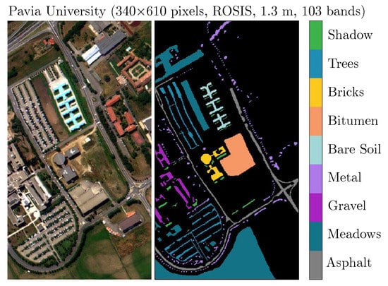
Figure 1.
The Pavia University scene captures nine classes of various spectral characteristics.
Table 2.
The number of samples (pixels) for each class in the Pavia University dataset.
2.1.2. Deep Mars
The Deep Mars [23] model uses deep learning to identify various types of objects, such as craters, sand dunes, streaks, and edges, present on the surface of Mars (see examples rendered in Figure 2). The dataset was annotated by crowdsourcing where the authors developed a web application that allows people to manually tag the objects present in the images. Such a model can be helpful in research concerning the evolution of the landscapes of our solar system but could also be leveraged during the autonomous spacecraft landing, provided the host-device throughput would be sufficient to run the model in real-time. Deep Mars can be adapted to classify similar objects present on the surfaces of other celestial objects, e.g., using transfer-learning techniques. Given that the model has to be deployed on satellites, it is important that one optimizes it to work on edge-like devices that have constrained hardware and power requirements.
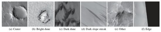
Figure 2.
Example input images of each category for Deep Mars model.
Table 3 shows the Deep Mars architecture. Being a classification task, it is a natural choice to use a variation of CNNs. The authors have adapted the AlexNet image classifier [24] by removing the final fully connected layer and re-defining the output classes to classify images from Mars. The authors claim the model gives an accuracy of 94.5% over the testing dataset. The model uses grayscale high-resolution images collected by a HiRISE (High-Resolution Imaging Science Experiment) camera for the Mars Reconnaissance Orbiter. The original stripe-shaped pictures of a spatial resolution of 30 cm per pixel were manually reviewed seeking the objects of interest: craters, bright dunes, dark dunes, dark slope streaks, others, and edges. These findings were then cropped out and rescaled to create a sole image classification dataset, where each sample can be described by a single label. The possible labels and image quantities belonging to each class are presented in Table 4.
Table 3.
The Deep Mars architecture utilized for classifying Mars images. The bolded layers have been added during the model reshaping, as discussed in the following part of the manuscript (Section 3).
Table 4.
The number of samples (images) for each label in the Deep Mars dataset.
2.1.3. Deep Moon
Deep Moon leverages the previous work by Silburt [25]. It is a two-step crater detection system, consisting of (i) a deep learning model for image segmentation and (ii) a template matching algorithm (discussed further) to localize the craters in the segmentation mask. It can automatically process datasets collected from lunar exploration campaigns. Therefore, it functions as a baseline for us to improve in terms of adapting the original model to be more efficient and deployable in edge devices. More broadly, the results will have applications for efficient data analytics onboard robotic probes for space exploration missions.
A craters record and chronology are key for the exploration of the solar system. Traditionally, crater detection has been done manually via visual inspection of images. However, this approach is not practical for the vast numbers of small-sized craters on the moon. This model introduces a novel method to determine the position and size of craters from lunar digital elevations maps using CNNs. The dataset used to train the model corresponds to a digital elevation map (DEM) and the craters catalog. The moon’s DEM is a global raster with elevation data, generated by NASA and the Japanese Aerospace Agency with the spatial resolution of 118 m per pixel. The craters dataset corresponds to the combination of two human-generated craters catalogs: one contains craters with a diameter between 5 and 20 km, and the other encompasses craters with a diameter greater than 20 km. Finally, the images were generated by randomly cropping DEM mapping, so the number of craters in each image may vary from just one to a few dozens. Figure 3 shows the example input image, the output mask generated by the deep learning model, and the craters positions proposed by the template matching step.
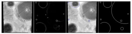
Figure 3.
Different stages of the Deep Moon detection system compared to the ground truth. Going from left: (i) input DEM image, (ii) output of the CNN model, (iii) craters detected by the template-matching-driven algorithm, (iv) ground truth.
Table 5 shows the Deep Moon architecture consisting of convolutional, pooling, dropout, and concatenate layers. The model is adapted from U-Net [26], which was originally designed for biomedical segmentation tasks. It is a fully-convolutional model consisting of the contracting and expanding paths, ultimately forming a U-shape. In the expanding path, each block receives the depth-matched feature maps from the contracting path using the skip connection; hence, the features can propagate through the architecture. The main differences between the vanilla U-Net and Deep Moon is the number of filters in the Conv2D layers and the addition of the dropout layers.
Table 5.
The Deep Moon architecture utilized for detecting Moon craters. All layers are connected sequentially with a few exceptions of additional skip-connections, specified in the “Attached” column. The bolded layers have been added during the model reshaping, as discussed in the following part of the manuscript (Section 3).
2.2. Deployment Toolchain
Vitis AI is a development environment platform for deploying AI inference models on hardware devices by Xilinx. It consists of optimized IP, tools, libraries, models, and example designs and enables the on-the-edge utilization of FPGA devices in embedded appliances, including satellite and aerospace devices [27]. Vitis AI can effectively deploy models created with popular AI libraries/frameworks, such as Caffe, PyTorch, and TensorFlow. The models undergo a series of steps, such as quantization and compilation, to be converted into a form that is deployable on the target embedded device. The architecture of an embedded device for AI acceleration according to the Xilinx model consists of:
- System-On-Chip (SoC) device, which has multi-core CPU and FPGA (as described in Appendix A).
- Deep Learning DPU IP (as described in detail in Appendix A).
- Linux-based operating system.
- Software interface and drivers for DPU IP provided by Xilinx (described in more details in the following Section 2.2.2).
- Software for loading, controlling, and running AI models (as described in the following Section 2.2.2).
To deploy a deep learning algorithm on an embedded device, practitioners have to support the inference process with data loading, pre- and post-processing, and storing the results. In the embedded application, the Xilinx libraries and runtime environment for establishing a connection with the DPU units are used. Both the application and the model are deployed on an embedded system containing an FPGA-based DPU and an ARM CPU running a Linux distribution. The embedded Linux distribution is built with PetaLinux [28] tools, provided by Xilinx, and based on the Yocto Project build system.
It is worth mentioning that both the hardware and software configurations can easily impact the capabilities and performance of the inference process. Not only the model parameters but also DPU and ARM-based systems can be configured and customized to achieve the best results. To trace and understand the entire process, the accuracy metrics of the model are measured, and this is done at each step of the deployment pipeline, which is shown in Figure 4. The consecutive Section 2.2.1 and Section 2.2.2 provide an in-depth description of each step of the process.
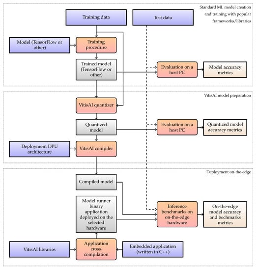
Figure 4.
Deployment pipeline of an AI model on an embedded device with Xilinx’s Vitis AI (nodes are color-coded: blue for inputs, red for actions, gray for artifacts, and yellow for results; some connections are dashed for visual clarity).
2.2.1. Preparing Deep Models for Deployment
The Vitis AI development environment comes with the benefit of being able to deploy deep models created with popular AI libraries/frameworks. As already mentioned, they include Caffee, PyTorch, and TensorFlow (both version 1 and 2). In this work, TensorFlow is utilized, but the deployment process for other frameworks is analogous. The models are created on standard PC machines using Python and trained (preferably) using GPUs. This process is the same as the common procedure of training AI models in the industry and does not require using any additional Xilinx tools.
To build a deployable deep model, one needs to exploit the compatible layers—the list of such layers is included in the Vitis Ai documentation [27] (see the deployment process visualized in Figure 4). These include but are not limited to convolutional layers, fully connected layers, different pooling layers, batch normalization layers, upsampling layers, and concatenation operations. Importantly, various layers may be subject to some parameters constraints to keep the compatibility with the Xilinx toolchain. Additionally, some layers (e.g., softmax and sigmoid) are compatible with the Xilinx toolchain but are not utilized by the DPU and instead delegated to the CPU.
Once the model is trained, it can be evaluated on the test subset (elaborating appropriate training/validation/test splits is application-dependent and should be done with care, as incorrectly determined subsets may lead to over-optimistic conclusions on the performance of deep models [22]). To fully track the model’s abilities, the quality metrics during the deployment are captured (for all intermediate models that are elaborated during this process). The model is then saved in a representation that is specific to the used Python AI library and can be deployed on an edge device.
Afterwards, the model trained in full precision is quantized and compiled—these operations transform it into a model graph representation that describes operations performed on the DPU to execute the inference process. Quantization and compilation are performed by the Vitis Ai tools, provided as command-line programs or Python modules, as previously, specific for a certain framework. The quantization process changes the internal representation of the model’s parameters during the inference [29]. Usually, standard computational platforms perform AI-related calculations on floating point data types (with varying precision depending on if the model is used on CPUs or GPUs). Since the DPU operates with a fixed precision, the models are adjusted (i.e., quantized) to perform operations on the DPU compatible 8-bit integer value types. The quantization task is run iteratively using a calibration dataset (being approx. 10% of the available training data, as suggested by Xilinx [27]), which is used to determine the range of input values and internal representations of the corresponding parameters. It is worth mentioning that an appropriate selection of the calibration set is pivotal, especially in the case of multi-source training samples. The quantized model can still be executed on a standard PC; hence, one can evaluate its performance using the unseen test samples, thus verifying the impact of the quantization process on the abilities of the underlying model.
Finally, the model is compiled and thus translated into a DPU-specific description of the operation flow. Because of that, this step is specific to the DPU architecture and requires passing the DPU footprint to succeed. Here, the non-compatible layers of the model may be disregarded—they have to be either delegated to the CPU or manually run on the DPU. In the case of the deep learning algorithms investigated in this work, the disregarded layers include softmax (Deep Earth and Deep Mars) and sigmoid (Deep Moon). The model preparation process may include some additional optimization steps, such as pruning the original deep architecture [30]. It may ultimately help us reduce the network’s size by eliminating, e.g., redundant parameters and/or connections in the model, which have minimal impact on the overall accuracy of the algorithm [29].
2.2.2. The Model Runner for Embedded Applications
The output of the compilation process is a deep model file containing the description of GPU utilization to perform the inference. However, this is not enough to run an inference on an embedded system. Therefore, an accompanying runner application is required to communicate with the DPU—it has to use Linux libraries and runtime to establish a connection with the DPU. These are available for C++ and Python programming languages [27,31].
For performance reasons, the C++ language was used to develop the embedded application. This means that the application has to be cross-compiled for the ARM CPU-based Linux running on the embedded system. Besides handling DPU communication and data loading, the app may also perform the operations delegated to the CPU. In the investigated case, the output softmax (Deep Earth, Deep Mars) and sigmoid (Deep Moon) operations are executed on the CPU. Interestingly, Vitis AI offers a possibility of manual softmax execution on DPU, which requires special hardware configurations—it might be beneficial to explore this possibility for models that extensively utilize such operations (here, softmax is calculated over small vectors; 9 values for Deep Earth, and 6 for Deep Mars). The sigmoid operation, which is used by Deep Moon, is not supported by DPU at this moment.
The implementation of data loading and DPU utilization is up to the developer of the embedded application. In the investigated case, the data are loaded by a single thread—this does not concern the MLPerf metrics since only the inference times are measured. However, this may be further optimized for the sake of real-life scenarios performance. The inference process and CPU-delegated layers calculations are, however, parallelized. Each MLPerf inference query is divided equally between CPU workers, where each worker owns a separate connection with the DPU. Furthermore, it is possible to create more CPU threads than DPU cores—in this case, the DPU cores are shared between the CPUs. The scheme enables the parallelization of CPU-delegated calculations; for example, some threads may calculate softmax operations while the others wait on the DPU. Multithreaded execution may additionally utilize heavier parallel read and write to the DPU, which is offered by Xilinx. Since the CPU workers send and receive data to the DPU sample by sample, it is pointless to run configurations with fewer CPU threads than DPU cores. (This fact has also been confirmed experimentally.)
2.3. The Benchmarking Scenarios and Metrics
The proposed benchmarking scenarios are built upon the approach introduced in MLPerf, and three test modes are utilized: Offline, Single-Stream, and Multi-Stream. Each mode supplies the inference system with data queries, where a single portion of data is sent to the inference system in various ways. A single query can contain an arbitrary number of samples depending on a given benchmarking scenario. One specific constraint imposed by MLPerf is that samples in each query must be in the contiguous memory layout, i.e., in the flat contiguous buffer. The size and dimension of a sample are dependent on the specific deep network architecture, e.g., it can be a 2D image or a single hyperspectral pixel. It is worth mentioning that the proposed benchmarking modes allow us to effectively capture a range of different real-life use cases in which the data are acquired using a single/multiple sensors and in which various levels of parallelization are possible.
Therefore, the following test modes to benchmark deep learning models are considered:
- Offline mode. In this mode, the entire dataset over which the inference will be performed is loaded into RAM at startup (thus, a single query is utilized). The total inference time is measured (excluding the data loading and prepossessing time). The performance metric becomes the sample throughput (samples per second). The offline mode benchmarks full performance under heavy load in scenarios where a large portion of data is gathered for the inference.
- Single-Stream mode. In this mode, one sample per query is sent to the inference system. The next query is not fed until the previous response has been received. The time of inference duration (or latency) is measured for each query, and the performance metric is the 90th percentile of latency to filter out the outlying values of this metric. The single-stream mode covers the streaming-like scenarios where the parallelization possibilities are limited because the samples come one at a time.
- Multi-Stream mode. In this scenario, a query of N samples is supplied in every time interval of length T, where T is benchmark-specific and also acts as the latency bound. If the inference system is available, it processes the incoming query. Otherwise, it delays the remaining queries by one interval. Here, no more than % of the queries may produce one or more skipped intervals to meet the Quality-of-Service (QoS) requirement. The performance metric becomes the integer value quantifying the number of streams that the system supports while meeting the QoS requirement. This mode is heavily parameterized and can be tested on multiple settings (with varying numbers of threads, querying interval, and more). The Multi-Stream mode measures real-time processing capabilities in situations where data from N sensors or a series of N images is to be processed in a single query per a given interval. The multi-stream mode investigates the online streaming capabilities in parallel environments, e.g., processing data captured using multiple sensors.
Each benchmarking scenario can be run per setup, being a combination of a specific deep network model running on a specific piece of hardware; hence, one can refer to a setup using a setup tuple, e.g., Deep Earth, PetaLinux 2020.1 distro, 1 Thread, 1 DPU core (frequency Hz, architecture), on Leopard DPU EVALB ZU9 model.
3. Experiments
The study is divided into three experiments (related to three different use cases) concerning HSI segmentation using Deep Earth (Section 3.1), classification of Mars images using Deep Mars (Section 3.2), and detection of craters on Moon using Deep Moon (Section 3.3). Here, the experimental settings are presented, and the results are discussed in detail. The models were coded in Python 3.8 with the TensorFlow 2.3 backend.
3.1. Use Case 1: Hyperspectral Image Segmentation Using Deep Earth
The training of the Deep Earth (using the ADAM optimizer [32] with the categorical cross-entropy loss, and the learning rate of , , and ) finished if after 15 consecutive epochs, the accuracy over the validation set ( of randomly picked training pixels) does not increase.
To quantify the performance of Deep Earth, the overall and balanced accuracy (OA and BA, respectively) for all classes, together with the values of the Cohen’s kappa , where and are the observed and expected agreement (assigned vs. correct label) and [33], are reported. To train the model, a dataset consisting of 225 samples per class was incorporated. All metrics are obtained for the remaining (unseen) test data. Note that this approach can be used for quantifying the classification performance of spectral CNNs without the training-test information leak that would have happened for spectral-spatial models, which utilize the pixel’s neighborhood information during the classification [22].
The initial approach consisted in exploiting 1-D convolutions within the spectral CNN. However, the current implementation of the Vitis AI TensorFlow 2 quantizer does not support any 1-D operations [30]; hence, all such layers were expressed in terms of 2-D convolutions. The model was thus recreated to fit the framework requirements without any significant impact on its abilities. In Table 6, the quality metrics captured for all versions of Deep Earth that were generated within the deployment pipeline (i.e., the original model trained and utilized in full precision, the model after quantization and compilation) are gathered. One can appreciate that all metrics are consistently very high without any significant performance deterioration across all versions of Deep Earth.
Table 6.
The change of metrics across different stages of Deep Earth deployment.
3.2. Use Case 2: Classification of Mars Images Using Deep Mars
Deep Mars was trained using 80% of the dataset (10% was held out for each validation and training sets). The data are available through the Jet Propulsion Laboratory webpage at https://pds-imaging.jpl.nasa.gov/, accessed on 30 September 2021. It was trained using an ADAM optimizer (categorical cross entropy loss), with a learning rate of and 32 samples per batch. The training was stopped after five epochs.
While deploying the original Deep Mars model (presented in Table 3), we encountered a compilation error that the maximum kernel size of a 2-D convolution was exceeded. According to the documentation, the Vitis AI compiler tries to optimize the (Flatten → Dense) connection by expressing the underlying operation as a 2-D convolution. Such an optimization, being reasonable from the mathematical point of view (since any dense layer can be expressed in terms of convolutions losslessly), introduces heavy restrictions on the scale of the operands (specifically: the size of the input tensor). To succeed, the convolutional kernel of the new artificial layer needs to fit the whole incoming tensor at once. Only then can it efficiently convolve over the dense layer weights, each time producing a single number (which, indeed, is a dot product between flattened input and the weights vector). The current Xilinx implementation does not allow disabling this behavior, yet the authors claim to remove the limitation of the kernel size in future releases.
For this experiment, the dimensionality of the tensor coming into the flattened layer was reduced, so two more sets of (convolution+pooling) layers were added before the flattened one (they are boldfaced on the architecture scheme, see Table 3). The weights of the initial layers were preserved, needing to retrain only the newly added (or modified) ones. Having the same training setup as for the original layer (except utilizing 9 epochs instead of 5), the accuracy was improved by about 5%. As a side effect, the number of trainable parameters of the model shrank by over 93%. The model could be compiled without any disruptions afterward. Although there is a visible drop in BA for the compiled Deep Mars model that is ready to be deployed on the edge device (Table 7), other classification metrics reveal that the deployed model still offers high-quality performance.
Table 7.
The change of metrics across the different stages of Deep Mars deployment.
3.3. Use Case 3: Detection of Craters on Moon Using Deep Moon
The Deep Moon model was trained with the subset of 30,000 training images, whereas the validation and test sets contained 5000 images each. The training process utilized the Adam optimizer (with the binary cross-entropy acting as the loss function), four epochs (with no early stopping), a learning rate of 0.0001, 0.15 dropout probability, and a batch size of 32 images.
The output of the CNN model is a mask of candidate craters’ edge locations. To create a list of detected craters with their spatial parameters (such as radius and coordinates), the mask needs to be quantized to 0–1 values at a given threshold and then processed by the template matching-based algorithm. The algorithm involves sliding rings of radii through the image in an iterative manner, seeking the areas for which the correlation with the ring is the highest. If the score exceeds a threshold (being a hyper-parameter of the algorithm that could be fine-tuned over the validation images), a crater of radius r in that location is registered. In case the neighboring pixels are also highly correlated, the dominant one is selected, whereas others are rejected in order to prevent registering multiple detections that all refer to the same crater. The process is depicted in Figure 5.
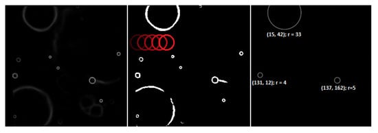
Figure 5.
The template matching algorithm utilized in the Deep Moon pipeline. The left image is the input (output of the CNN model). The middle one shows the already quantized mask with the ring sliding across the image (red). The right one shows locations of those craters, for which the correlation between the ring and the image at that place exceeded the threshold and was dominant in their neighborhood.
The very two-stage nature of the system (i.e., detection of crater candidates using a deep model, and then pruning false positives through template matching) compels the two-stage evaluation approach. Firstly, the quality of the segmentation masks generated by the CNN model using binary cross-entropy between the predicted and ground truth images is evaluated. It fulfills the role of being a loss function during training but does not provide much insight into the quantitative assessment of the spotted craters. For this purpose, the whole system after the template matching step using the Average Precision (AP) metric is evaluated.
Since the Deep Moon detection system differs from the traditional bounding-box-oriented approaches, the following way of calculating the metric in the Deep Moon case is utilized:
- Gather all predictions (correct and incorrect) over the whole test dataset and sort them according to their confidence level in descending order. The confidence of the detection is its correlation registered during the template matching. Note that only detections that have surpassed the template matching threshold and were dominant in their neighborhood are considered.
- Count the number of all (n) and correct (c) detections.
- Iteratively, for : calculate the current recall as: and the current precision as: . Note that the recall will slowly increase from 0 to 1 as correct detections increase.
- Plot the precision-recall plot and calculate the area under the curve (AUC). Opposite to recall, precision will act “chaotically” at first, (e.g., when the sequence of detections starts with a correct detection followed by an incorrect one), but the impact on AUC of such peaks is negligible.
To make the assessment exhaustive, the basic statistics, such as global recall (), global precision (), global F1-score (), and loss (binary cross entropy), are also attached. These, however, should be treated secondarily in the case of the object detection task. In Table 8, the metrics obtained for all versions of the Deep Moon model are gathered. As in the previous algorithms, the deployment process does not adversely affect the abilities of the technique. These experiments show that quantizing and compiling the model for the target edge device allow us to maintain high-quality operational capabilities of the algorithms in a variety of computer vision tasks.
Table 8.
The change of metrics across different stages of Deep Moon deployment.
In Figure 6, the examples of selected scenes (of varying complexity), together with the corresponding detections elaborated using the original deep model, are rendered (the false positives are annotated in green, whereas false negatives are in red; additionally, the corresponding quality metrics are presented). Note that the number of craters in the input images can significantly vary. However, the algorithm’s performance does not seem to be impaired by numerous detections in a single frame. Such qualitative analysis can help better understand the capabilities of the algorithms in image analysis tasks and should be an important part of any experimental study [34].
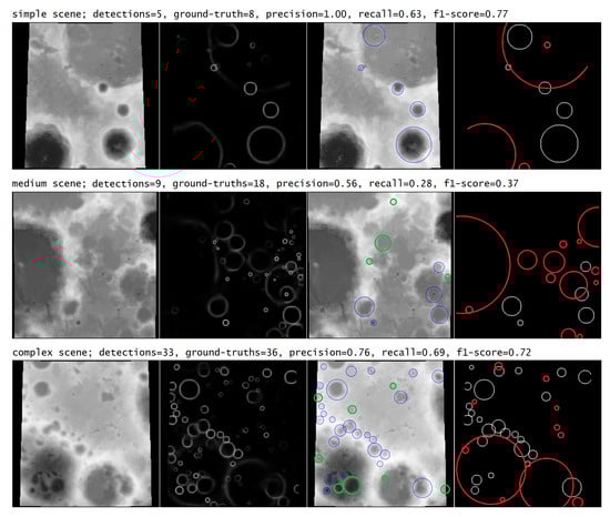
Figure 6.
Examples of correct and incorrect predictions made for scenes of varying complexity. Going from the left: (i) input image, (ii) output of the model, (iii) craters detected by the template-matching step (false positives are rendered in green), and (iv) the ground truth (false negatives are in red).
3.4. Benchmarking Hardware Architectures for On-Board Processing
As stated in Section 2.3, the MLPerf-inspired benchmarks (with different scenarios) are performed for models deployed on the edge hardware (Section 2.2)—note that the device can be configured in different ways, as discussed later in this section. However, running the benchmarks on an on-the-edge device imposes additional memory constraints, as the memory capacities are much smaller than those of standard workstations. For this reason, the test sets have to be limited in size in order to fit in RAM (this is especially important for the Offline mode, where the entire dataset has to be loaded into a continuous memory region). Since the Deep Mars test set contains only 382 samples, it is copied three times in order to extend the benchmarking time. Overall, the test sets included 40,526 samples for Deep Earth, 1146 samples for Deep Mars, and 500 for Deep Moon. Even though these numbers are much smaller than recommended by MLPerf, they are specific to the hardware constraints. Finally, the idle power consumption of Leopard is slightly over 12 W without any energy-saving optimizations. The Multi-Stream scenario is parameterized by the time interval value T. MLPerf suggests this parameter to be 50 ms, which was used for Deep Mars and Deep Moon. However, Deep Earth, which is a fairly small CNN, can reach a very high number of streams processed in 50 ms. Hence, the interval value of 5 ms for Deep Earth was used to keep the benchmark execution time reasonable.
Given the available hardware resources, a subset of possible DPU configurations for the benchmarks was selected. It includes the most parallelized versions of the simplest B512 architecture—4 × B512 (with 4 CPU threads) and 6 × B512 (with 6 CPU threads). For the intermediate architecture B1024, the 2 × B1024 (with 2 and 4 CPU threads), 4 × B1024 (with 4 CPU threads), and 6 × B1024 (with 6 CPU threads) configurations are used. The most powerful B4096 DPU setup is utilized in 1 × B4096 (1, 2, and 4 CPU threads), 2 × B4096 (2 and 4 CPU threads), and 3 × B4096 (3 and 6 CPU threads) parallelization variants. The 6 × B512, 6 × B1024, and 3 × B4096 architectures are the most complex configurations that can be synthesized on the Leopard DPU.
The benchmarking results are gathered in Table 9, Table 10 and Table 11 (Offline mode), Table 12, Table 13 and Table 14 (Single-Stream mode), and in Table 15, Table 16 and Table 17 (Multi-Stream mode). The peak power consumption values for each benchmark are summarized in Table 18, Table 19 and Table 20. The experimental results are presented for each deep learning algorithm, DPU architecture, and the number of CPU threads.
Table 9.
Offline benchmark results (throughput in samples per second) for the B512 DPU architecture. Here, OOM denotes out of memory.
Table 10.
Offline benchmark results (throughput in samples per second) for B1024 DPU architecture.
Table 11.
Offline benchmark results (throughput in samples per second) for B4096 DPU architecture.
Table 12.
Single-Stream benchmark results (90-percentile latency bound) for B512 DPU architecture.
Table 13.
Single-Stream benchmark results (90-percentile latency bound) for B1024 DPU architecture.
Table 14.
Single-Stream benchmark results (90-percentile latency bound) for B4096 DPU architecture.
Table 15.
Multi-Stream benchmark results (max number of streams) for B512 DPU architecture.
Table 16.
Multi-Stream benchmark results (max number of streams) for B1024 DPU architecture.
Table 17.
Multi-Stream benchmark results (max number of streams) for B4096 DPU architecture.
Table 18.
The peak power consumption during benchmarks for B512 DPU architecture.
Table 19.
The peak power consumption during benchmarks for B1024 DPU architecture.
Table 20.
The peak power consumption during benchmarks for B4096 DPU architecture.
One can appreciate the fact that using more advanced DPU architectures results in larger throughput values in the Offline mode. For example, see 6 × B1024 vs. 6 × B512 (both with 6 CPU threads) for Deep Mars—it results in 46% better throughput per second (Table 9 and Table 10). This is universal to all models; however, the increase may vary between the models and DPUs. Here, when comparing 4 × B1024 and 4 × B512, one can observe the 16% improvement for Deep Earth, 51% for Deep Mars, and 92% for Deep Moon (all with 4 CPU threads; Table 9 and Table 10). It indicates that larger models benefit more from the complex hardware architectures. Additionally, exploiting the DPUs with more inference cores also improves the throughput. One can notice that utilizing 4 × B1024 instead of 2 × B1024 improves the metric by 70% for Deep Mars (both configurations with 4 CPU threads; Table 10). An increase in the number of cores may lead to a nearly directly proportional increase in performance. For example, 3 × B4096 (3 CPU threads) vs. 2 × B4096 (2 CPU threads) vs. 1 × B4096 (1 CPU thread) leads to gains of 187% and 99% of throughput for Deep Moon (Table 11).
Increasing the number of CPU threads often leads to an improvement in throughput. For the 2 × B4096 architecture, changing the number of threads from 2 to 4 increases the throughput by 21% for Deep Earth, by 39% for Deep Mars, and 9% for Deep Moon (Table 11). However, using too many CPU threads in regard to the available DPU cores can lead to worse throughput, as many CPU threads can compete for DPU access at the same time and various problems, such as starvation may occur. For example, for the 1 × B4096 architecture, using 4 threads instead of 2 leads to slight decrease in throughput for all models (Table 11). The best throughput for Deep Earth was obtained for the 6 × B1024 architecture with 6 CPU threads (Table 10). In the case of Deep Mars and Deep Moon, the best Offline results were achieved with 3 × B4096 (6 CPU threads for Deep Mars and 3 for Deep Moon) architecture (Table 11). Deep Moon, being the most complex network, demands a lot of memory to establish connections with the DPU. For the configurations with the largest number of threads, there was not enough space to allocate memory for the DPU connections. This problem was marked as OOM (out-of-memory) in the tables.
The Single-Stream metrics also benefit from more advanced architectures. Table 12, Table 13 and Table 14 show that the more complex architectures lead to smaller values of latency. Since this mode processes sample by sample (one at a time), it does not benefit from parallelization. Thus, increasing the number of DPU cores and CPU threads does not improve latency. Using more CPU cores leads to a slight increase in the Single-Stream metrics, as the number of parallel threads increases while they are of no use. The best Single-Stream results for all networks were achieved by the single threaded configuration of the most complex 4 × B4096 architecture (with a single CPU thread; Table 14).
The Multi-Stream scenario metrics scale similarly to the Offline ones. Utilizing better DPU architectures, more DPU cores, and CPU threads increases the number of streams. Going from the 1 × B1024 (1 CPU thread) to 2 × B1024 (2 CPU threads) architecture yields a doubled stream number for Deep Mars and 72% increase for Deep Earth (Table 16). The slight decrease in the metrics for 1 × B4096 with four CPU threads is visible (Table 17). The best Multi-Stream score for Deep Earth was achieved with 6 × B1024 and 6 CPU threads configuration (Table 16). For Deep Mars, the largest stream number was obtained for the 3 × B4096 architecture with 6 CPU threads (Table 17). One can observe that Deep Moon is not able to deliver real-time operation with the given time interval of 50 ms. Interestingly, the number of streams for 6 × B512 and 3 × B4096 (both with 6 CPU threads) was the same (Table 15 and Table 17). When comparing these two results in the Offline mode, 6 × B512 achieves slightly better throughput (Table 9 and Table 11). Both of these are the configurations with the largest number of cores for the selected DPU architectures. However, 6 × B512 uses 16% less power in peak while performing better than 3 × B4096 (Table 18 and Table 20). With smaller network architectures, it may be more beneficial to use simpler DPU cores than fewer intricate ones (when parallel processing is considered).
The power consumption raises with the number of DPU cores and DPU architecture complexity. More advanced models are also more power demanding—while the peak power for Deep Earth with 6 × B1024 (6 CPU threads) and 3 × 4096 (6 CPU threads) is nearly the same, it raises over 27% for Deep Mars (Table 19 and Table 20). The peak power consumption for all models was highest when using the most intricate 3 × B4096 DPU architecture (Table 20). Additionally, measuring the operations per second on the DPU was done using Xilinx tools—the maximum performance was achieved for Deep Moon with 3 × b3096 architecture and 3 CPU threads. The DPU peaked at 1.094182 TOP/s (tera-operations per second) per core (over 3 TOP/s total).
The benchmarks indicated that Deep Moon is not able to operate in real-time within a 50 ms time interval. However, the U-Net architecture was not designed with real-time operations in mind. Usually, real-time computer vision systems utilize specific network architectures optimized for fast inference, such as YOLO [35], Fast R-CNN [36], and RetinaNet [37]. Importantly, Vitis AI is able to exploit such networks for more efficient real-time tasks (there is a YOLO-v3 example provided by Xilinx).
One can observe that using multiple CPU threads is beneficial to speed up the inference process. However, some notes about possible CPU starvation in regard to fewer DPU cores were made. The extra threads in the system may be exploited in different ways to utilize DPU potential as best as possible. Finally, a more advanced parallelization scheme may be used to achieve better inference.
4. Conclusions and Future Work
An unprecedented level of success of deep learning has triggered its fast adoption in virtually all areas of science and various industries. The same route is followed in space applications, related to Earth observation, autonomy of satellites, or anomaly detection from telemetry data captured once the spacecraft is operating in orbit. Since transferring large amounts of data back to Earth, e.g., as in the case of the satellites equipped with hyperspectral imagers, is time-consuming and costly, moving the processing on-board the spacecraft has become an important research topic nowadays, especially given that there exists high-performance hardware, which can be used in orbit. Therefore, verifying and validating artificial intelligence techniques before deploying them in such constrained execution environments are critical to fully understand their functional and non-functional capabilities.
To tackle the problem of thorough verification and validation of deep learning algorithms in space applications, an end-to-end benchmarking approach that allows practitioners to capture the most important quality metrics that relate to the performance abilities of the underlying models, as well as to their inference characteristics was introduced. The experiments showed that the introduced technique that benefits from the widely-used Xilinx tools is model-agnostic and straight-forward to use for any deep learning model. We believe that such benchmarking should become a standard tool for rigorously verifying the algorithms before deploying them in the wild. It could make the adoption of state-of-the-art deep learning faster in on-board satellite data analysis faster; thus, it could be an important step towards exploiting deep learning at the edge in various applications, in both critical and non-critical missions. Finally, when coupled with the data-level digital twins that enable us to simulate on-board image acquisition [20], the proposed benchmarking technique can become a comprehensive tool for assessing the robustness of on-board AI through various simulations.
Although the deep learning deployment chain allows us to fit a deep model into the target hardware, there exist several techniques that may be used to further optimize such models for on-board processing. Our current research efforts are focused on utilizing knowledge distillation approaches for making deep models more resource-frugal and better fitted to the underlying hardware [38]. Furthermore, the existing deep learning models could be further improved through pruning unnecessary (or redundant) parts of the architecture— Xilinx claims up to 90% parameters reduction during the pruning process in the built-in deep network pruning tool [27]. Finally, it will be interesting to analyze not only inference time and efficiency but also the time required for the data loading and pre/post-processing, as these steps are commonly used in the machine learning-powered processing pipelines. Here, it may be beneficial to use the excess CPU power for parallel data loading. Therefore, the problem of the “optimal” utilization of the CPU and DPU resources remains an interesting research challenge that should be tackled by both machine learning and embedded hardware communities.
Author Contributions
Conceptualization, J.N., M.G., M.Z., D.J. and R.D.; methodology, J.N., M.G., M.Z., D.J. and R.D.; software, M.Z., P.B. and G.G.; validation, M.Z., P.B., M.M., G.G., M.G. and J.N.; investigation, M.Z., P.B., M.M., G.G., M.G., J.P., K.B., D.J., R.D. and J.N.; data curation, M.Z., P.B., M.M., J.P., K.B., D.J. and J.N.; writing—original draft preparation, M.Z., P.B., G.G., M.G., D.J., R.D. and J.N.; visualization, M.Z. and P.B.; supervision, J.N. and R.D.; funding acquisition, J.N. and R.D. All authors have read and agreed to the submitted version of the manuscript.
Funding
This work was partially funded by the European Space Agency (the GENESIS project), and supported by the ESA -lab (https://philab.phi.esa.int/). The work was supported by the Polish National Centre for Research and Development under Grant POIR.01.01.01-00-0356/17. J.N. was supported by the Silesian University of Technology grant for maintaining and developing research potential. We acknowledge the support of the Canadian Space Agency (CSA). This project activity is undertaken with the financial support of the Canadian Space Agency.
Institutional Review Board Statement
Not applicable.
Informed Consent Statement
Not applicable.
Data Availability Statement
Data Availability Statement: Publicly available datasets were analyzed in this study. This data can be found here (accessed on 30 September 2021): Deep Earth: http://www.ehu.eus/ccwintco/index.php/Hyperspectral_Remote_Sensing_Scenes, https://hyperspectral.ee.uh.edu/, Deep Mars: https://pds-imaging.jpl.nasa.gov/search/?fq=-ATLAS_THUMBNAIL_URL%3Abrwsnotavail.jpg&q=*%3A*, Deep Moon: https://zenodo.org/record/1133969.
Conflicts of Interest
The authors declare no conflict of interest.
Abbreviations
The following abbreviations are used in this manuscript:
| AI | Artificial Intelligence |
| AP | Average Precission |
| ARM | Advanced RISC Machines |
| AUC | Area under the curve |
| BA | Balanced Accuracy |
| CNN | Convolutional Neural Network |
| CPU | Central Processing Unit |
| DCDC | Direct Current-Direct Current (converter) |
| DDR4 | Double Data Rate 4 |
| DEM | Digital Elevation Map |
| DNN | Deep Neural Network |
| DPU | Deep Learning Processing Unit |
| FPGA | Field Programmable Gate Array |
| GPU | Graphics Processing Unit |
| HSI | Hyperspectral Imaging |
| HiRISE | High Resolution Imaging Science Experiment |
| JTAG | Joint Test Action Group |
| ML | Machine Learning |
| MPSSE | Multi-Protocol Synchronous Serial Engine |
| OA | Overall Accuracy |
| OOM | Out Of Memory |
| PC | Personal Computer |
| PMOD | Peripherial module interface |
| PU | Pavia University (dataset) |
| QSPI | Quad Serial Peripherial Interface |
| QoS | Quality of Service |
| R-CNN | Recurrent Convolutional Neural Network |
| RAM | Random Access Memory |
| RELU | Rectified Linear Unit |
| SATA | Serial AT Attachment |
| SoC | System on a Chip |
| SoM | System on Module |
| TF | TensorFlow |
| UART | Universal Asynchronous Receiver-Transmitter |
Appendix A. The Hardware
The benchmarks were carried out on the Leopard DPU Evalboard Model (the block diagram is shown in Figure A1, whereas a physical board is presented in Figure A2). The evaluation board is the Leopard DPU flavor designed to support benchmarking and software tests in laboratory conditions in contrast to the Flight configuration described in [39]. The Evalboard Model uses a single Trenz TE0808 SoM (system on module) as a central part. It exposes identical interfaces as Flight configuration of Leopard DPU (interfaces are connected to the same FPGA banks and use the same voltages). The board consists of:
- Trenz TE0808 module (XCZU09EG) with 4 GB of DDR4 and built-in QSPI boot Flash memory.
- Exposed single 1 GbE Ethernet interface.
- XCZU09EG can boot from QSPI, microSD, Ethernet, NAND, or JTAG.
- Exposed 16-line LVDS interface; it is able to handle external image sensors or other data providers.
- Up to two SATA-III Solid State Drives in M.2 factor.
- Custom board controller that allows to fully control the board by PC (power control and monitoring, Linux UART, high-speed data transmission)—it allows using the board in fully automated Hardware-In-The-Loop tests.
- DCDC converters that convert single external power supply voltage in the range of 9–13 V.
- 4 GB of embedded NAND flash.
- Exposed one USB 2.0 interface (XCZU09EG as a host or on-the-go).
- 4 PMOD sockets routed to PL (one differentially routed).
- Exposed AURORA interface—it can be used to connect two boards together via high-speed synchronous Gigabit Transceiver GTH interface directly connected to FPGA GTH transceivers.
- Over temperature protections and a fan controller.
- Exposed Display Port.
- CAN full-speed interface.
- High-speed two-way synchronous series communication (e.g., to connect external radio module).
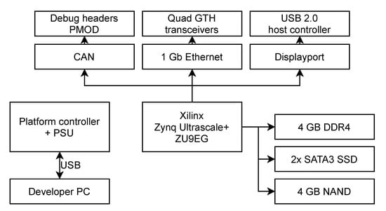
Figure A1.
The block diagram of the KP Labs Leopard DPU Evalboard used for laboratory benchmarks.
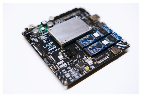
Figure A2.
The physical KP Labs Leopard DPU Evalboard Model used for laboratory benchmarks.
The Xilinx Deep Learning Processing Unit is a configurable computation engine optimized for convolutional neural networks. It can be implemented in the FPGA programmable logic (PL) portion of XCZU09EG SoM, which is present on the Leopard Evalboard. The degree of parallelism utilized in the engine is a design parameter and can be selected according to the target device and application. It is integrated in the FPGA portion of SoC and connects to CPU and RAM memory by the AXI interfaces. The main principle of DPU is to behave as a co-processor, having its instructions and scheduler. The DPU settings and its parallelism (multiple IPs can be integrated in one design, if the size and timing constrains allow for doing that) are one of the main design and optimization decisions that need to be undertaken. Here, the following settings during the models’ evaluation are considered:
- The number of DPU IPs (1–6). One can incorporate multiple DPU IPs, allowing for parallel processing of the input samples. Up to 6 DPUs were used (where FPGA size and timing budget allowed). For the largest DPU (B4096), only 3 IP cores fitted inside FPGA.
- The DPU Architectures: B512, B1024, B4096. There are multiple dimensions of parallelism in the DPU convolution unit. The different DPU architectures require different programmable logic resources. The larger architectures can achieve higher performance with more resources and more parallelized calculations.
On the other hand, the following settings remain unchanged during the experimentation:
- Clocks: 300 and 600 MHz (clk and clk2x).
- UltraRAM: disabled.
- DRAM: disabled.
- RAM usage: low.
- Channel Augmentation: enabled.
- DepthwiseConv: enabled.
- AveragePool: enabled.
- RELU type: RELU+LeakyRelu+ReLU6.
- DSP48 usage: high.
- Low power: disabled.
For more detailed explanation of DPU architectures and parameters refer to [40].
References
- Arechiga, A.P.; Michaels, A.J.; Black, J.T. Onboard Image Processing for Small Satellites. In Proceedings of the IEEE National Aerospace Electronics Conference, NAECON, Dayton, OH, USA, 23–26 July 2018; pp. 234–240. [Google Scholar]
- Bahl, G.; Daniel, L.; Moretti, M.; Lafarge, F. Low-Power Neural Networks for Semantic Segmentation of Satellite Images. In Proceedings of the 2019 International Conference on Computer Vision Workshop, ICCVW 2019, Seoul, Korea, 27–28 October 2019; pp. 2469–2476. [Google Scholar]
- Denby, B.; Lucia, B. Orbital Edge Computing: Machine Inference in Space. IEEE Comput. Archit. Lett. 2019, 18, 59–62. [Google Scholar] [CrossRef]
- Wang, Y.; Yang, J.; Guo, X.; Qu, Z. Satellite Edge Computing for the Internet of Things in Aerospace. Sensor 2019, 19, 4375. [Google Scholar] [CrossRef] [PubMed] [Green Version]
- Zhang, C.; Chan, J.; Li, Y.; Li, Y.; Chai, W. Satellite Group Autonomous Operation Mechanism and Planning Algorithm for Marine Target Surveillance. Chin. J. Aeronaut. 2019, 32, 991–998. [Google Scholar] [CrossRef]
- Bohm Agostini, N.; Dong, S.; Karimi, E.; Torrents Lapuerta, M.; Cano, J.; Abellán, J.L.; Kaeli, D. Design Space Exploration of Accelerators and End-to-End DNN Evaluation with TFLITE-SOC. In Proceedings of the 2020 IEEE 32nd International Symposium on Computer Architecture and High Performance Computing (SBAC-PAD), Porto, Portugal, 9–11 September 2020; pp. 10–19. [Google Scholar]
- Reddi, V.J.; Cheng, C.; Kanter, D.; Mattson, P.; Schmuelling, G.; Wu, C.J. The Vision Behind MLPerf: Understanding AI Inference Performance. IEEE Micro 2021, 41, 10–18. [Google Scholar] [CrossRef]
- Boutros, A.; Nurvitadhi, E.; Ma, R.; Gribok, S.; Zhao, Z.; Hoe, J.C.; Betz, V.; Langhammer, M. Beyond Peak Performance: Comparing the Real Performance of AI-Optimized FPGAs and GPUs. In Proceedings of the International Conference on Field-Programmable Technology, (IC)FPT 2020, Maui, HI, USA, 9–11 December 2020; pp. 10–19. [Google Scholar]
- Varghese, B.; Wang, N.; Bermbach, D.; Hong, C.H.; Lara, E.D.; Shi, W.; Stewart, C. A Survey on Edge Performance Benchmarking. ACM Comput. Surv. 2021, 54, 1–33. [Google Scholar] [CrossRef]
- Dinelli, G.; Meoni, G.; Rapuano, E.; Benelli, G.; Fanucci, L. An FPGA-Based Hardware Accelerator for CNNs Using On-Chip Memories Only: Design and Benchmarking with Intel Movidius Neural Compute Stick. Int. J. Reconfigurable Comput. 2019, 2019, 7218758. [Google Scholar] [CrossRef] [Green Version]
- Hao, T.; Huang, Y.; Wen, X.; Gao, W.; Zhang, F.; Zheng, C.; Wang, L.; Ye, H.; Hwang, K.; Ren, Z.; et al. Edge AIBench: Towards Comprehensive End-to-End Edge Computing Benchmarking. In International Symposium on Benchmarking, Measuring and Optimization; Lecture Notes in Computer Science; Springer: Cham, Switzerland, 2019; pp. 23–30. [Google Scholar] [CrossRef] [Green Version]
- Caldas, S.; Wu, P.; Li, T.; Konečný, J.; McMahan, H.B.; Smith, V.; Talwalkar, A. LEAF: A Benchmark for Federated Settings. arXiv 2018, arXiv:1812.01097. [Google Scholar]
- Bianco, S.; Cadene, R.; Celona, L.; Napoletano, P. Benchmark Analysis of Representative Deep Neural Network Architectures. IEEE Access 2018, 6, 64270–64277. [Google Scholar] [CrossRef]
- Mattson, P.; Cheng, C.; Coleman, C.; Diamos, G.; Micikevicius, P.; Patterson, D.; Tang, H.; Wei, G.Y.; Bailis, P.; Bittorf, V.; et al. MLPerf Training Benchmark. arXiv 2019, arXiv:1910.01500. [Google Scholar]
- Reuther, A.; Michaleas, P.; Jones, M.; Gadepally, V.; Samsi, S.; Kepner, J. Survey and Benchmarking of Machine Learning Accelerators. In Proceedings of the 2019 IEEE High Performance Extreme Computing Conference, HPEC 2019, Waltham, MA, USA, 24–26 September 2019; pp. 1–9. [Google Scholar]
- Wang, Y.; Wang, Q.; Shi, S.; He, X.; Tang, Z.; Zhao, K.; Chu, X. Benchmarking the Performance and Energy Efficiency of AI Accelerators for AI Training. In Proceedings of the 20th IEEE/ACM International Symposium on Cluster, Cloud and Internet Computing, CCGRID 2020, Melbourne, VIC, Australia, 11–14 May 2020; pp. 744–751. [Google Scholar]
- Furfaro, R.; Bloise, I.; Orlandelli, M.; Di Lizia, P.; Topputo, F.; Linares, R. Deep Learning for Autonomous Lunar Landing. Adv. Astronaut. Sci. 2018, 167, 3285–3306. [Google Scholar]
- Engineering, I.; Way, E.J.E.R.; Engineering, I.; Way, E.J.E.R. Lunar Landing. pp. 1–16. Available online: https://arc.aiaa.org/doi/10.2514/6.2020-1910 (accessed on 30 September 2012).
- Zhang, J.; Xia, Y.; Shen, G. A Novel Deep Neural Network Architecture for Mars Visual Navigation. arXiv 2018, arXiv:1808.08395. [Google Scholar]
- Nalepa, J.; Myller, M.; Cwiek, M.; Zak, L.; Lakota, T.; Tulczyjew, L.; Kawulok, M. Towards On-Board Hyperspectral Satellite Image Segmentation: Understanding Robustness of Deep Learning through Simulating Acquisition Conditions. Remote Sens. 2021, 13, 1532. [Google Scholar] [CrossRef]
- Nalepa, J.; Myller, M.; Kawulok, M. Transfer Learning for Segmenting Dimensionally Reduced Hyperspectral Images. IEEE Geosci. Remote Sens. Lett. 2020, 17, 1228–1232. [Google Scholar] [CrossRef] [Green Version]
- Nalepa, J.; Myller, M.; Kawulok, M. Validating Hyperspectral Image Segmentation. IEEE Geosci. Remote Sens. Lett. 2019, 16, 1264–1268. [Google Scholar] [CrossRef] [Green Version]
- Wagstaff, K.L.; Lu, Y.; Stanboli, A.; Grimes, K.; Gowda, T.; Padams, J. Deep Mars: CNN Classification of Mars Imagery for the PDS Imaging Atlas. In Proceedings of the 32nd AAAI Conference on Artificial Intelligence, AAAI 2018, New Orleans, LA, USA, 2–7 February 2018; pp. 7867–7872. [Google Scholar]
- Krizhevsky, A.; Sutskever, I.; Hinton, G.E. ImageNet Classification with Deep Convolutional Neural Networks. In Proceedings of the Advances in Neural Information Processing Systems 25: 26th Annual Conference on Neural Information Processing Systems 2012, Lake Tahoe, NV, USA, 3–6 December 2012; 2012; pp. 1106–1114. [Google Scholar]
- Silburt, A.; Ali-Dib, M.; Zhu, C.; Jackson, A.; Valencia, D.; Kissin, Y.; Tamayo, D.; Menou, K. Lunar Crater Identification via Deep Learning. Icarus 2019, 317, 27–38. [Google Scholar] [CrossRef] [Green Version]
- Weng, W.; Zhu, X. INet: Convolutional Networks for Biomedical Image Segmentation. IEEE Access 2021, 9, 16591–16603. [Google Scholar] [CrossRef]
- Xilinx. Vitis AI User Guide; Technical Report UG1414 (v1.4); Xilinx: San Jose, CA, USA, 2021. [Google Scholar]
- Xilinx. PetaLinux Tools Documentation, Reference Guide; Technical Report UG1144 (v2021.1); Xilinx: San Jose, CA, USA, 2021. [Google Scholar]
- Liang, T.; Glossner, J.; Wang, L.; Shi, S.; Zhang, X. Pruning and Quantization for Deep Neural Network Acceleration: A Survey. Neurocomputing 2021, 461, 370–403. [Google Scholar] [CrossRef]
- Xilinx. Vitis AI Optimizer User Guide; Technical Report UG1333 (v1.4); Xilinx: San Jose, CA, USA, 2021. [Google Scholar]
- Xilinx. Vitis AI Library User Guide; Technical Report UG1354 (v1.4); Xilinx: San Jose, CA, USA, 2021. [Google Scholar]
- Kingma, D.P.; Ba, J. Adam: A Method for Stochastic Optimization. arXiv 2014, arXiv:1412.6980. [Google Scholar]
- McHugh, M.L. Interrater Reliability: The Kappa Statistic. Biochem. Medica 2012, 22, 276–282. [Google Scholar] [CrossRef]
- Wu, Y.; Wan, G.; Liu, L.; Wei, Z.; Wang, S. Intelligent Crater Detection on Planetary Surface Using Convolutional Neural Network. In Proceedings of the 2021 IEEE 5th Advanced Information Technology, Electronic and Automation Control Conference (IAEAC), Chongqing, China, 12–14 March 2021; Volume 5, pp. 1229–1234. [Google Scholar]
- Redmon, J.; Divvala, S.; Girshick, R.B.; Farhadi, A. You Only Look Once: Unified, Real-Time Object Detection. In Proceedings of the 2016 IEEE Conference on Computer Vision and Pattern Recognition (CVPR), Las Vegas, NV, USA, 26 June–1 July 2016; pp. 779–788. [Google Scholar]
- Girshick, R. Fast R-CNN. In Proceedings of the 2015 IEEE International Conference on Computer Vision (ICCV), Santiago, Chile, 11–18 December 2015; pp. 1440–1448. [Google Scholar]
- Lin, T.Y.; Goyal, P.; Girshick, R.; He, K.; Dollár, P. Focal Loss for Dense Object Detection. IEEE Trans. Pattern Anal. Mach. Intell. 2020, 42, 318–327. [Google Scholar] [CrossRef] [Green Version]
- Gou, J.; Yu, B.; Maybank, S.J.; Tao, D. Knowledge Distillation: A Survey. Int. J. Comput. Vis. 2021, 129, 1789–1819. [Google Scholar] [CrossRef]
- Nalepa, J.; Kuligowski, P.; Gumiela, M.; Drobik, M.; Nowak, M. Leopard: A New Chapter in On-Board Deep Learning-Powered Analysis of Hyperspectral Imagery. In Proceedings of the 2020 IAC, IAF Earth Observation Symposium, Online, 12–14 October 2020; pp. 1–8. [Google Scholar]
- Xilinx. DPUCZDX8G for Zynq UltraScale+ MPSoCs, Product Guide; Technical Report PG338 (v3.3); Xilinx: San Jose, CA, USA, 2021. [Google Scholar]
Publisher’s Note: MDPI stays neutral with regard to jurisdictional claims in published maps and institutional affiliations. |
© 2021 by the authors. Licensee MDPI, Basel, Switzerland. This article is an open access article distributed under the terms and conditions of the Creative Commons Attribution (CC BY) license (https://creativecommons.org/licenses/by/4.0/).