Article

Evaluation of Deep Learning Segmentation Models for Detection of Pine Wilt Disease in Unmanned Aerial Vehicle Images

1
National Research Center of Intelligent Equipment for Agriculture, Beijing Academy of Agricultural and Forestry Sciences, Beijing 100097, China
2
Beijing Key Laboratory of Intelligent Equipment Technology for Agriculture, Beijing Academy of Agricultural and Forestry Sciences, Beijing 100097, China
3
Beijing Research Center of Intelligent Equipment for Agriculture, Beijing Academy of Agricultural and Forestry Sciences, Beijing 100097, China
4
National Center for International Research on Agricultural Aerial Application Technology, Beijing Academy of Agricultural and Forestry Sciences, Beijing 100097, China
5
Shandong Ruida Pest Control Company Limited, Jinan 250000, China
*
Author to whom correspondence should be addressed.
Contributed equally to this work.
Remote Sens. 2021, 13(18), 3594; https://doi.org/10.3390/rs13183594
Submission received: 15 June 2021 / Revised: 29 August 2021 / Accepted: 1 September 2021 / Published: 9 September 2021
(This article belongs to the Special Issue Thematic Information Extraction and Application in Forests)

Abstract

:
Pine wilt disease (PWD) is a serious threat to pine forests. Combining unmanned aerial vehicle (UAV) images and deep learning (DL) techniques to identify infected pines is the most efficient method to determine the potential spread of PWD over a large area. In particular, image segmentation using DL obtains the detailed shape and size of infected pines to assess the disease’s degree of damage. However, the performance of such segmentation models has not been thoroughly studied. We used a fixed-wing UAV to collect images from a pine forest in Laoshan, Qingdao, China, and conducted a ground survey to collect samples of infected pines and construct prior knowledge to interpret the images. Then, training and test sets were annotated on selected images, and we obtained 2352 samples of infected pines annotated over different backgrounds. Finally, high-performance DL models (e.g., fully convolutional networks for semantic segmentation, DeepLabv3+, and PSPNet) were trained and evaluated. The results demonstrated that focal loss provided a higher accuracy and a finer boundary than Dice loss, with the average intersection over union (IoU) for all models increasing from 0.656 to 0.701. From the evaluated models, DeepLLabv3+ achieved the highest IoU and an F1 score of 0.720 and 0.832, respectively. Also, an atrous spatial pyramid pooling module encoded multiscale context information, and the encoder–decoder architecture recovered location/spatial information, being the best architecture for segmenting trees infected by the PWD. Furthermore, segmentation accuracy did not improve as the depth of the backbone network increased, and neither ResNet34 nor ResNet50 was the appropriate backbone for most segmentation models.

1. Introduction

Pine wilt disease (PWD) induced by pinewood nematode, Bursaphelenchus xylophilus, is the most harmful threat to pine forests and responsible for huge ecological and economic losses in China [1,2]. Although the pathogenesis of PWD remains unclear, research has found that the accumulation of terpenes in xylem tissue results in cavitation, interrupting the water flux in pine trees [3,4]. Infected pines wilt and die quickly (e.g., between two to three months) and no action can be taken to save them. The pinewood nematode is native to North America (USA and Canada). It was first detected in Japan at the beginning of the 20th century and in the 1970s in China [5,6]. The spread of PWD is rapid because of the lack of natural enemies. Until 2020, the presence of PWD has been reported in 18 provinces (718 counties and cities) in China, and more than 600 million pines have been killed [7].
The pinewood nematode is transmitted by pine sawyer beetles, which fly quickly and freely between pines [8,9]. Hence, PWD quickly spreads and destroys numerous pines. As no method has been devised to treat infected pines, the best way to reduce the spreading speed and coverage of the PWD is to identify infected trees early and cut them down as soon as possible. Research on early identification or warning of PWD has been mainly focused on selecting the characteristic spectrum band, which is the band sensitive to PWD [10,11]. Although many studies have attempted to determine effective selection using ground high-spectral cameras or spectrometers, the complexity of the PWD spread still hinders early warning [12].
Pinewood nematodes often infringe on pine over large areas. Compared with manual field surveys, satellite and airborne remote sensing (including unmanned aerial vehicles [UAVs]) imaging provides faster acquisition of regional data to identify suspected pine trees infected with PWD (we use “infected pines” for short) [13,14,15]. As pinewood nematodes are too small to be identified in satellite remote sensing or UAV images, current methods based on these data for PWD identification often rely on the change of spectral reflectance of pines. Infected pines wilt in a few months, and their color is notably different from that of uninfected pines. White et al. [16] used 4 m multispectral IKONOS data and an unsupervised clustering method (ISODATA) to monitor the activation of pinewood nematodes. Hicke and Logan [17] used multitemporal QuickBird data to monitor and evaluate PWD. While satellite data can provide the regional distribution of PWD, their limited resolution restricts PWD monitoring at the scale of individual pines.
UAVs equipped with different cameras and flying at appropriate altitudes can obtain diverse images with high spatiotemporal resolutions under different weather conditions [18]. Hence, UAV imaging is currently one of the best methods to obtain data for PWD monitoring. Iordache et al. [19] used airborne spectral imagery equipment mounted on a UAV to obtain high-resolution multispectral and hyperspectral data of pines. Then, they adopted an algorithm based on random forests to identify infected pines. Syifa et al. [20] used an UAV to collect RGB (red-green-blue) color images and an artificial neural network and a support vector machine to detect candidate PWD-infected pines, achieving accuracies of 79.33% and 86.59% for evaluation in Wonchang.
Compared with traditional machine learning (ML), deep learning (DL) based on deep artificial neural networks provides the highest performance for image segmentation and object detection [21,22,23,24,25]. Thus, DL is also used in PWD monitoring, mainly with semantic segmentation and object detection models. Object detection models, such as the faster region convolutional neural network and You Only Look Once version 3 with variety backbones, have been widely applied for PWD identification [26,27,28,29]. These models can provide object-level detection of infected pines, but only define bounding boxes around the detected pines. Compared with semantic segmentation, object detection lacks sufficient boundary (shape) or size information, which is essential to evaluate the PWD damage, determine the number of infected pines, and plan the removal of infected pines [15]. Although semantic segmentation can provide detailed information of infected pines, few studies on PWD identification using semantic segmentation are available [30]. Thus, semantic segmentation models for PWD monitoring have not been thoroughly evaluated.
We evaluate various semantic segmentation models for extracting infected pines from UAV images and determine their performance. First, we collect experimental data over a large area using an UAV and annotate the training set containing infected pines. Then, we conduct a comprehensive performance evaluation of semantic segmentation models for PWD identification. Finally, we determine appropriate backbones and segmentation models for PWD identification.

2. Dataset

2.1. Study Area

Figure 1 displays the study area, north of Laoshan District, Qingdao, China. The land area of Laoshan is 395.79 km2 with a mean altitude of 360 m and highest altitude 1132.7 m. The temperature in the study area is suitable for sawyer beetles to live given the annual mean ground temperature of approximately 14.2 °C and annual mean precipitation of 660 mm. The land cover type is artificial coniferous forest, and the dominant type of vegetation is the black pine and Pinus densiflora. Most pines in this area are older than 70 years. The PWD was first found in this area before 2010. Four areas, Wanggezhaung (A1), Heihushan (A2), Huamuliu (A3), and Wangzijian (A4) in Laoshan, were selected as the experimental area (see the green aerial photography lines in Figure 1). The areas for A1, A2, A3, and A4 were 33.97 km2, 38.26 km2, 52.83 km2, and 35.37 km2, respectively.

2.2. UAV Image Collection

We used a fixed-wing UAV, DB-2 (Dabai Technology Co. Ltd.; China), which had strong wind resistance and a long service life. The maximum takeoff weight and maximum endurance time of the aircraft were 30 kg and 4 h, respectively. The camera for UAV imaging was the Sony Alpha 7R II (Sony Group Corporation, Japan), which is a 35 mm full-frame device with a maximum resolution of 7952 × 4472 pixels.
UAV imaging was conducted from 6 October to 14 October 2018. We collected the images in October, considering the feature of infected pines was more obvious. Pines are often infected in May due to the frequent activity of Longicorn, and most infected pines wilt in October when the other deciduous tree and healthy pines are still green. During data collection, no haze or clouds were observed, and the wind was mild. The UAV maintained an altitude below 700 m and a speed of 100 km/h. Equal-distance shooting was applied. The overlap along the flying direction was at least 75%, and the lateral overlap was at least 50%. Finally, an image resolution of 8 cm was obtained. After finishing data collection, we obtained 7586 images for the areas, with 1568, 1447, 2136, and 2435 images from Heihushan, Wanggezhaung, Wangzijian, and Huamuliu, respectively.

2.3. Field Survey

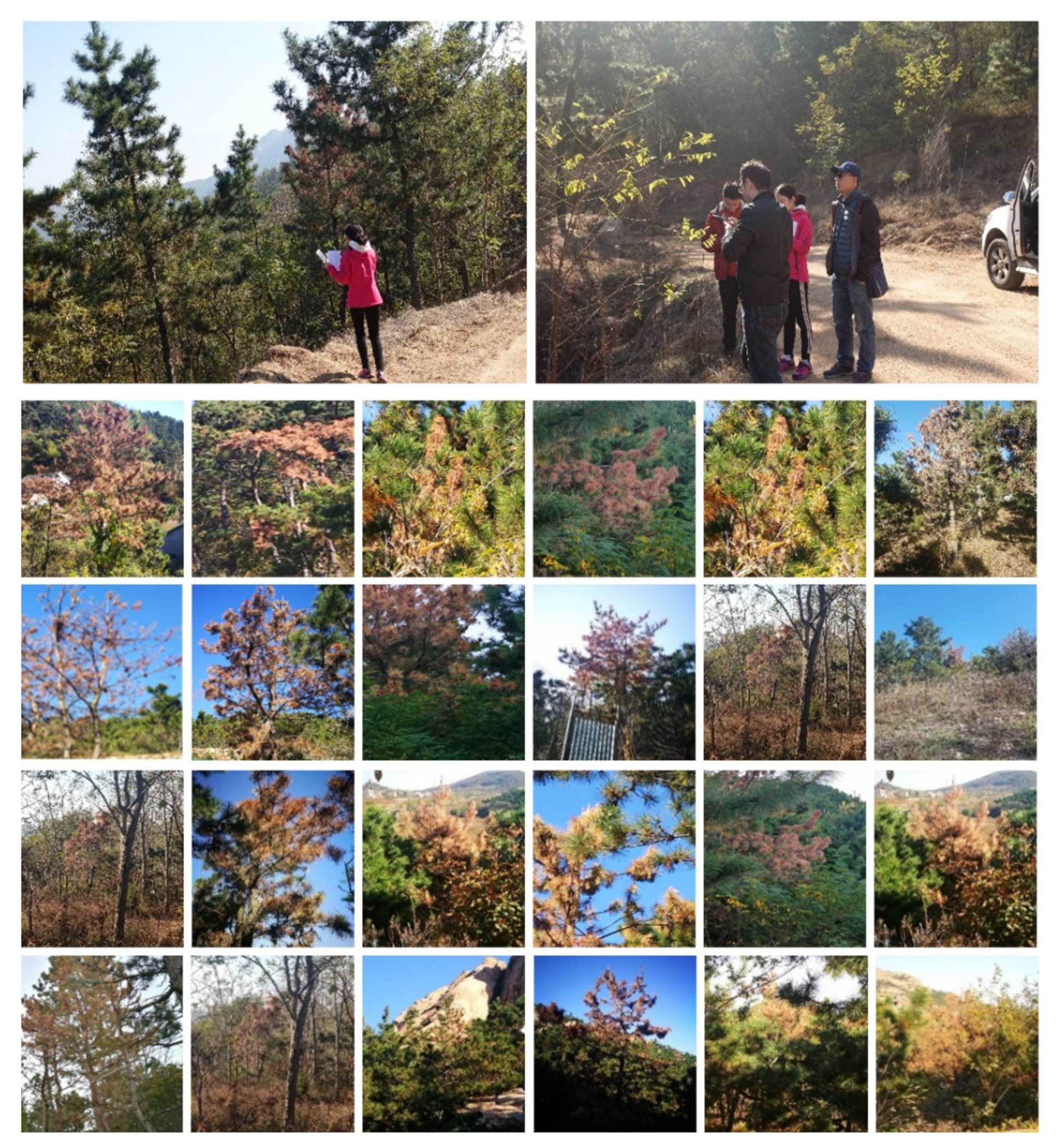
The field survey aimed at collecting images of different infected pine trees and constructing interpretation knowledge about the identification of infected pines on the UAV images. The field survey was conducted from 27 October to 31 October 2018. In the survey, telescopes, cameras, and a Global Navigation Satellite System device G190, which is made by UniStrong, China with an accuracy of 3–5 m, were used. The survey area was selected as that with higher density of infected pines. When an infected pine was found, we captured images of the pine and recorded the global positioning system information. In the field survey, we checked 185 infected pines and collected 706 images. Figure 2 displays images from the field survey and infected pines.

2.4. Data Annotation and Processing

To obtain high-quality training samples, the identification accuracy of infected pines from UAV images should be guaranteed. Therefore, we first validated the accuracy of manual interpretation. Specifically, we selected 200 UAV images that fully covered the ground field survey area. Then, we identified infected pines considering the ground field survey results. Overall, 179 of 185 (approximately 97.0%) infected pines were correctly identified. Thus, manual interpretation provided a high accuracy.
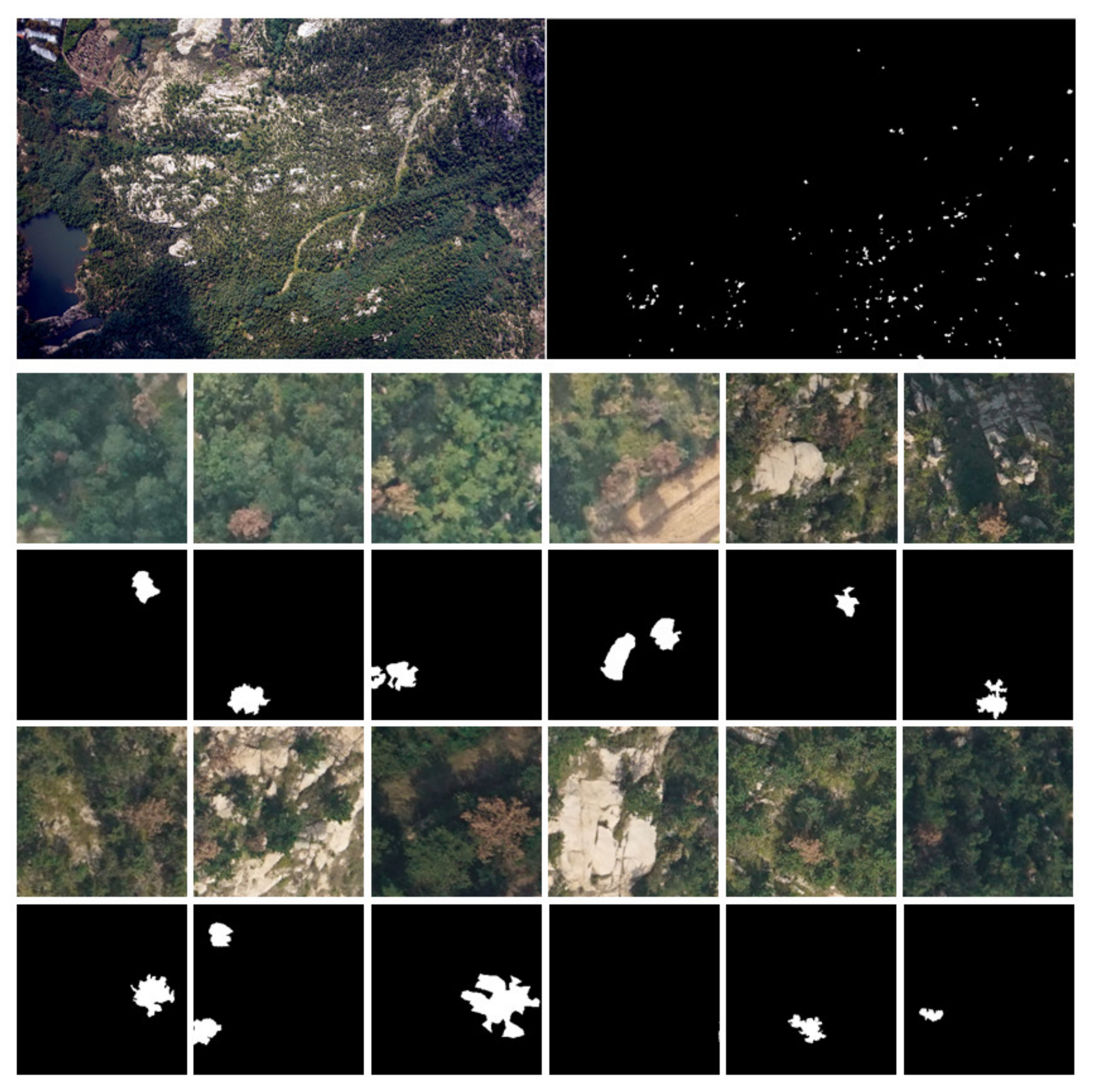
Then, we selected representative UAV images and annotated the corresponding labels. We collected 7586 UAV images for the four areas, but most images did not include any infected pines, and large overlaps between neighboring images were observed. Thus, we only selected 45 UAV images with a resolution of 7952 × 4472 pixels. Figure 1 displays detailed distributions of these images. The selected images included a variety of backgrounds (e.g., water, buildings, rocks, farmland, and trees). The total number of selected images for each area were 12, 7, 15, and 11 for A1, A2, A3, and A4, respectively. The annotation was performed using a region of interest tool from ENVI (version 5 from Harris Geospatial Solutions, Inc.; Broomfield, CO, USA). After annotation, 2352 infected pines were identified (see Figure 3).
We generated training samples from annotated images as follows. First, 200 images with a resolution of 256 × 256 pixels were clipped from an UAV image with a resolution of 7952 × 4472 pixels, and each clipped image included pixels of infected pines. Then, the annotated full-resolution image was rotated by 5°, 10°, and 15°, and for each rotated image, 200 images were clipped randomly. We did not change the brightness of the image because there were some mountain shadows in the UAV images (image in Figure 3, top-left corner). Overall, 36,000 samples with a resolution of 256 × 256 pixels were obtained. We split the obtained samples into 50% for training, 20% for validation, and 30% for testing.

3. Methods

3.1. Models

By examining DL applied to computer vision, we evaluated models constructed based on different concepts (see Table 1). These models were divided into four types:
  • Milestone segmentation fully convolutional networks (FCNs) for semantic segmentation [31].
  • Multiscale feature fusion models using pyramid pooling or symmetric encoders–decoders, such as PSPNet, U-Net, and SegNet [32,33,34].
  • Models using dilated convolution to increase the receptive field, such as DeepLabv3 and DenseASPP [35,36,37].
  • Models using a self-attention mechanism instead of multiscale feature fusion to capture contexts, such as DANet and OCNet [38,39].
An FCN is a milestone segmentation model, in which the output from pooling layer pool5 is up-sampled and fused with another pooling result to obtain a detailed feature map. The fully connected layer from the classification model is converted into a convolutional layer, turning the FCN into an end-to-end pixel-to-pixel network. Different upsampling ratios result in different resolutions (e.g., FCN-32s, FCN-16s, and FCN-8s). Here, we selected FCN-8s as the testing model as it provided the best location information.
U-Net is a widely used DL model for image segmentation, first intended for biomedical image segmentation. U-Net is derived from the FCN but applies two paths, constituting the U-shape architecture. The first path is an encoder that captures the context in the image at different scales. The encoder is a traditional stack of convolutional and max-pooling layers. The second path is a decoder that fuses data from the encoder and enables precise localization for segmentation.
PSPNet uses a pyramid parsing module to exploit global context information by context aggregation from different regions. Local and global features were combined to increase the final prediction reliability. PSPNet achieved a mean intersection over union (IoU) of 85.4% and 80.2% on PASCAL Visual Object Classes Challenges 2012 and the Cityscapes dataset, respectively.
DeepLabv3 is a representative DL model that uses dilated convolutions for semantic image segmentation. The dilated convolution increases the receptive field without downsizing the feature maps. In DeepLabv3, an augmented atrous spatial pyramid pooling (ASPP) module is implemented to detect convolutional features at multiple scales and obtain image-level features that encode the global context. DeepLabv3+ is based on the ASPP module and adds an encoder–decoder architecture to improve the performance and obtain fine boundaries.
DANet and OCNet use a self-attention mechanism, which is an important method to capture context and can accurately integrate local features with their global dependencies into multiscale feature fusion. Remarkably, DANet uses two types of attention modules in the spatial and channel dimensions on top of the traditional dilated FCN to capture and integrate contexts at different scales. DANet achieved a mean IoU of 81.5% on the Cityscapes dataset.

3.2. Loss Function and Model Training

We used two types of loss functions, the Dice loss [40] and focal loss [41], to handle imbalanced classes. The Dice loss was based on the Dice coefficient, defined as:
D i c e = 2 × A B A + B
where A B represented the pixels in both prediction A and ground truth B, and A and   B represented the numbers of pixels in A and B, respectively.
In cross-entropy, parameter α t was used to handle imbalanced classes, but its value did not differentiate between simple and complex examples. Alternatively, in the focal loss, term 1 p t γ allowed focus of the model on complex misclassified examples, as follows:
F L p t = α t 1 p t γ l o g p t
p t = p ,   i f   y = 1 1 p ,   o t h e r w i s e
where F L p t was the focal loss, α t and γ weighting factors with α t 0 ,   1   and   γ 0 ,   5 , p the model prediction with p 0 ,   1 , y the ground truth with y ± 1 , and p t the model prediction for the positive/negative class.
The models listed in Table 1 were implemented in the PyTorch 1.8 library. All the models were trained and tested on a workstation running Ubuntu 16.04. The workstation was equipped with an NVIDIA Tesla P100 graphics processor with 16 GB memory and an Intel Xeon 863 processor with 12 cores and 64 GB memory. The Adam optimizer with a learning rate of 0.001 was used, and no additional function was used to change the learning rate during training. A batch size of eight was used for each model, and training proceeded for 100 epochs.

3.3. Evaluation Metrics

We used metrics such as the precision, recall, Jaccard index, and F1 score to evaluate the performance of the different DL models. Precision indicated the ability of a classifier not to label a sample as positive that was negative. Recall evaluated the ability of the classifier to find all positive samples. For precision and recall, the best value was 1, and the worst 0. The Jaccard index, also called IoU or Jaccard similarity coefficient, was defined as the size of the intersection divided by the size of the union of two label sets. The Jaccard index ranged from 0 to 1, with 0 indicating no overlap and 1 indicating perfectly overlapping segmentation. The F1 score, also called Dice similarity coefficient, was the harmonic mean of the precision and recall. Its range was [0, 1], with 1 indicating perfect precision and recall, and 0 indicating zero precision or recall. Although common for imbalanced datasets, we did not use the overall accuracy in the evaluation.
The abovementioned metrics were calculated as:
R e c a l l = T P T P + F N
  J A , B = A B A B = A B A + B A B
P r e c i s i o n = T P T P + F P
F 1 = 2 P r e c i s i o n × R e c a l l P r e c i s i o n + R e c a l l
where T P represented the true positives (positive labels correctly predicted as positive), TN the true negatives (negative labels correctly predicted as negative), FP the false positives (negative labels incorrectly predicted as positive), FN the false negatives (positive labels incorrectly predicted as negative), and J A , B the Jaccard index between prediction A and ground truth B for a class.

4. Results

During training of each DL model, the model settings providing the highest performance (i.e., maximum F1 score of validation) were selected for evaluation. We trained each model five times to find the highest-performing settings, which were applied to the model on the test set to obtain the IoU, F1 score, precision, and recall (see Table 2). DeepLabv3+ achieved the best IoU and F1 score among the evaluated models. DeepLabv3 and DenseASPP demonstrated similar precision, and U-Net provided the best recall. As the IoU and F1 score reflected both precision and recall, they were more comprehensive metrics. Thus, DeepLabv3+ with the Dice loss demonstrated the highest overall performance among the evaluated models.
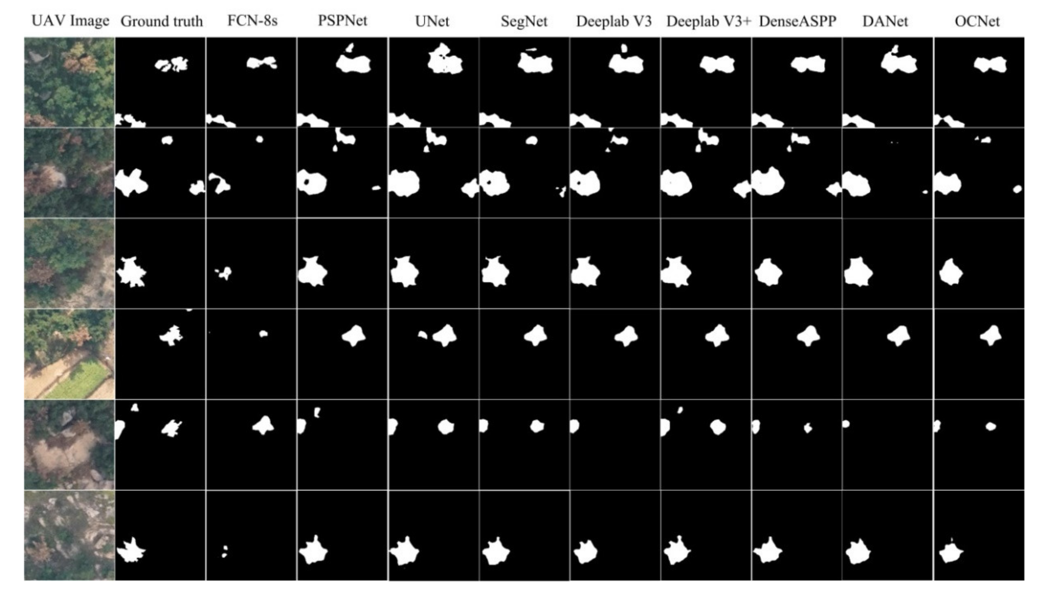
Figure 4 displays examples that illustrate how the evaluated models segmented infected pines. The first column is the input UAV image for prediction, and the second column displays the annotated ground truth of the infected pines. The third to eleventh columns display the predictions of each model using Dice loss. The input UAV images in Figure 4 display diverse objects. The first two rows mainly display healthy pines (green) and infected pines, being an easy scene for accurate prediction. The third and fourth rows display healthy pines, infected pines, soil, and crops (farmland), being more complex for prediction than the images in the first two rows. The images in the fifth and sixth rows display complex objects, including rocks, healthy pines, infected pines, and soil. The color of infected pines in these images was similar to the background, being more difficult to distinguish infected pines compared with the other images.
Figure 4 demonstrates that all the models suitably detected infected pines, and no background objects were falsely recognized as infected pines. Nevertheless, some models missed various pixels corresponding to infected pines, while others misclassified uninfected pines as infected ones. For instance, FCN-8s, DANet, and OCNet often missed more pixels of infected pines, and U-Net, PSPNet, and SegNet provided several false positives. Remarkably, FCN-8s predicted the smallest area of infected pines, especially for the images in the fourth and sixth rows. However, U-Net misclassified pixels corresponding to uninfected pines as indicating infected pines, as in the images in the first and second rows. While no models missed considerable infected pines, the predicted boundaries were inaccurate, but a detailed boundary was important to obtain the morphological characteristics of infected pines.
Table 3 lists the metrics obtained from the models trained with focal loss. All the models outperformed those trained with Dice loss. The mean IOU for all the models presented the highest improvement, increasing from 0.656 to 0.701, followed by precision; whereas the recall metric displayed the lowest improvement. The improvement difference between precision and recall indicated that the focal loss increased the segmentation accuracy of more positive samples (i.e., infected pines) than negative samples (i.e., background).
The FCN displayed the lowest improvement, whereas PSPNet provided a notable improvement. This might be because FCN-8s used a simple up-sampling method, and coarse features were obtained in the final convolutional layer. Among the evaluated models, DeepLabv3+ presented the highest performance with IoU and F1 scores of 0.720 and 0.832, respectively, followed by DenseASPP with IoU and F1 scores of 0.717 and 0.831, respectively. We considered four types of models:
  • Milestone segmentation FCNs, with multiscale feature fusion using pyramid pooling or symmetric encoder–decoder.
  • Multiscale feature fusion models using pyramid pooling or symmetric encoders–decoders.
  • Models using dilated convolution to increase the receptive field and ASPP for multiscale feature fusion.
  • Self-attention mechanism for multiscale feature fusion.
From them, using dilated convolution to enlarge the receptive field and obtain multiscale feature fusion provided a higher accuracy than other methods for segmenting infected pines.
Figure 5 displays segmentation results for each model on the test set. The models provided a fine segmentation boundary and were close to the ground truth. For models that tended to falsely identify background as infected pines (e.g., U-Net and PSPNet), the focal loss reduced the number of false positives. For models that missed more pixels of infected pines (e.g., FCN-8s and DANet), the focal loss increased the number of detected pixels corresponding to infected pines. However, for FCN-8s, although infected pines were more completely detected, this model missed some infected pines, such as the infected pines at the lower right corner of the image in the second row and that on the left side of the image in the fifth row.
The weighted cross-entropy used parameter α t to handle imbalanced classes but could not differentiate between simple and complex samples. Although Dice loss allowed for the handling of imbalanced classes, it could not focus on complex samples, being similar to cross-entropy. However, focal loss added term 1 p t γ to consider complex misclassified samples. Hence, it allowed imbalanced classes while increasing the ability to detect small objects and those difficult to classify. Therefore, focal loss results in finer boundaries than Dice loss. For example, the images in the first and sixth rows of Figure 5 demonstrate substantially improved results for the segmented boundary and detailed shapes of infected pines, while the corresponding results in Figure 4 present coarse boundaries and inaccurate shapes of infected pines.

5. Discussion

The experimental results demonstrated that DeepLabv3+ achieved the highest segmentation accuracy for identifying PWD-infected pines. Similar to other models, DeepLabv3+ is comprised of feature extraction (backbone) and fusion. As we used the same backbone for most models, the abovementioned performance differences were mainly attributable to feature fusion. Here, we further compared the effect of the backend on the segmentation performance for infected pines. To reduce the computation time, we only selected the highest-performing models for each type, namely, PSPNet, DeepLabv3+, and OCNet; then, we evaluated ResNet with increasing depths (i.e., ResNet34, ResNet50, ResNet101, and ResNet152) as backbones.
Table 4 lists the corresponding results. The performance of the models decreased as the depth of the ResNet backbone increased. Specifically, the IoU and F1 score decreased as the network depth of ResNet increased, whereas the precision increased. These trends suggested that the models demonstrated overfitting as the depth of ResNet increased, and the models did not gain accuracy from an increasing depth. Therefore, for segmenting infected pines in UAV images, the ResNet50 or ResNet34 backbone was sufficiently accurate to extract representative features.
Table 3 indicates that DeepLabv3+ considerably outperformed DeepLabv3 despite the small difference in architecture. Specifically, DeepLabv3+ added a decoder to further fuse high- and low-level features, thus obtaining a more detailed boundary. To clarify the effect of the decoder on model performance, we tested DeepLabv3 and DeepLabv3+ with different backbones (see Table 5).
DeepLabv3+ with the decoder outperformed DeepLabv3 for different ResNet depths, with the ResNet34 backbone achieving the highest accuracy to segment infected pines. The overall IoU of DeepLabv3+ increased by 1.94% compared with DeepLabv3, which had no decoder.
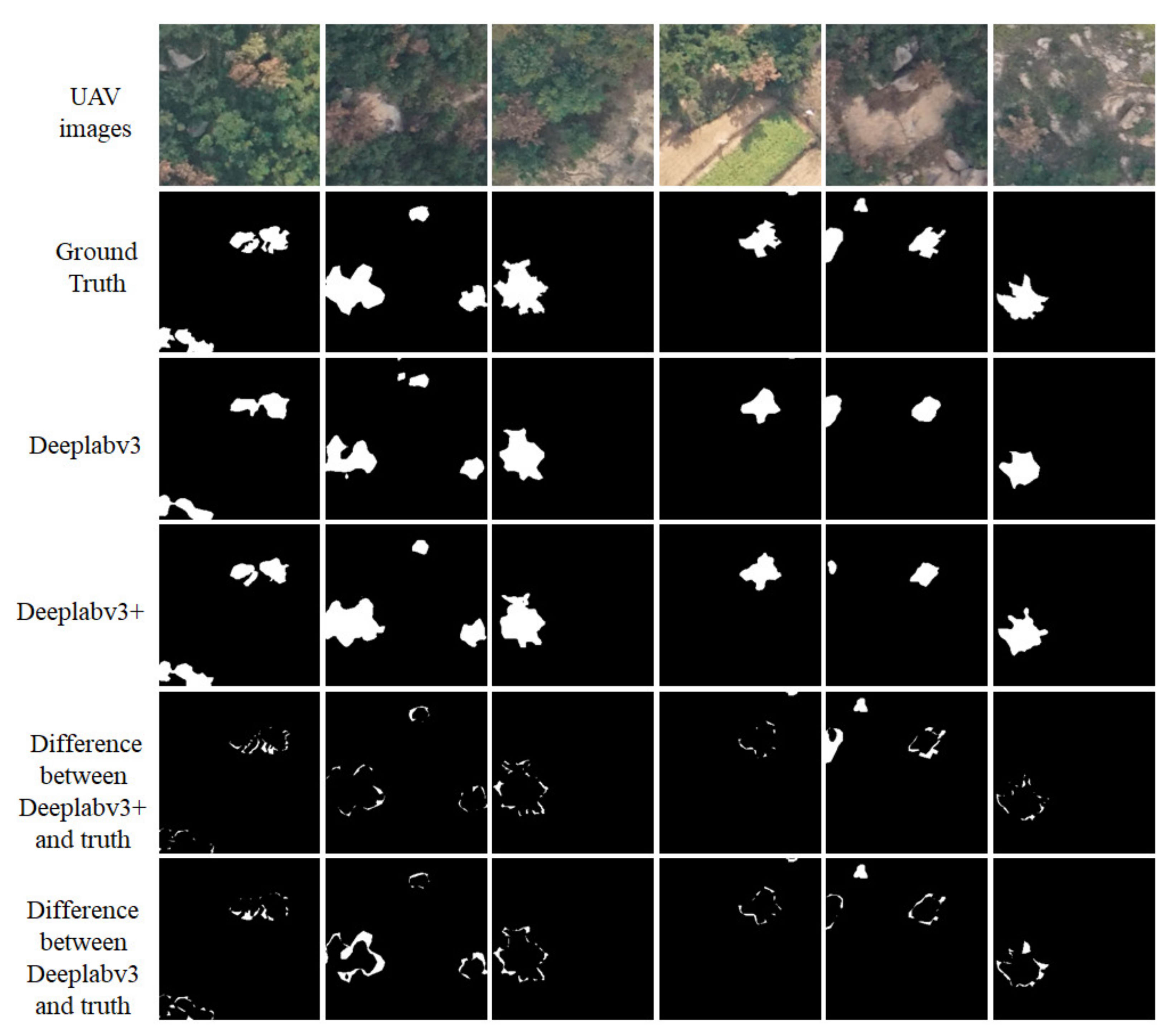
Figure 6 displays the difference between segmenting the results of DeepLabv3 and DeepLabv3+ using the highest-performing ResNet34 backbone. The white pixels in the fifth and sixth rows represented the segmentation results of DeepLabv3+ and DeepLabv3 subtracted from the ground truth, respectively. Compared with DeepLabv3, DeepLabv3+ segmenting was closer to the ground truth, providing a finer boundary, which was achieved by the decoder.
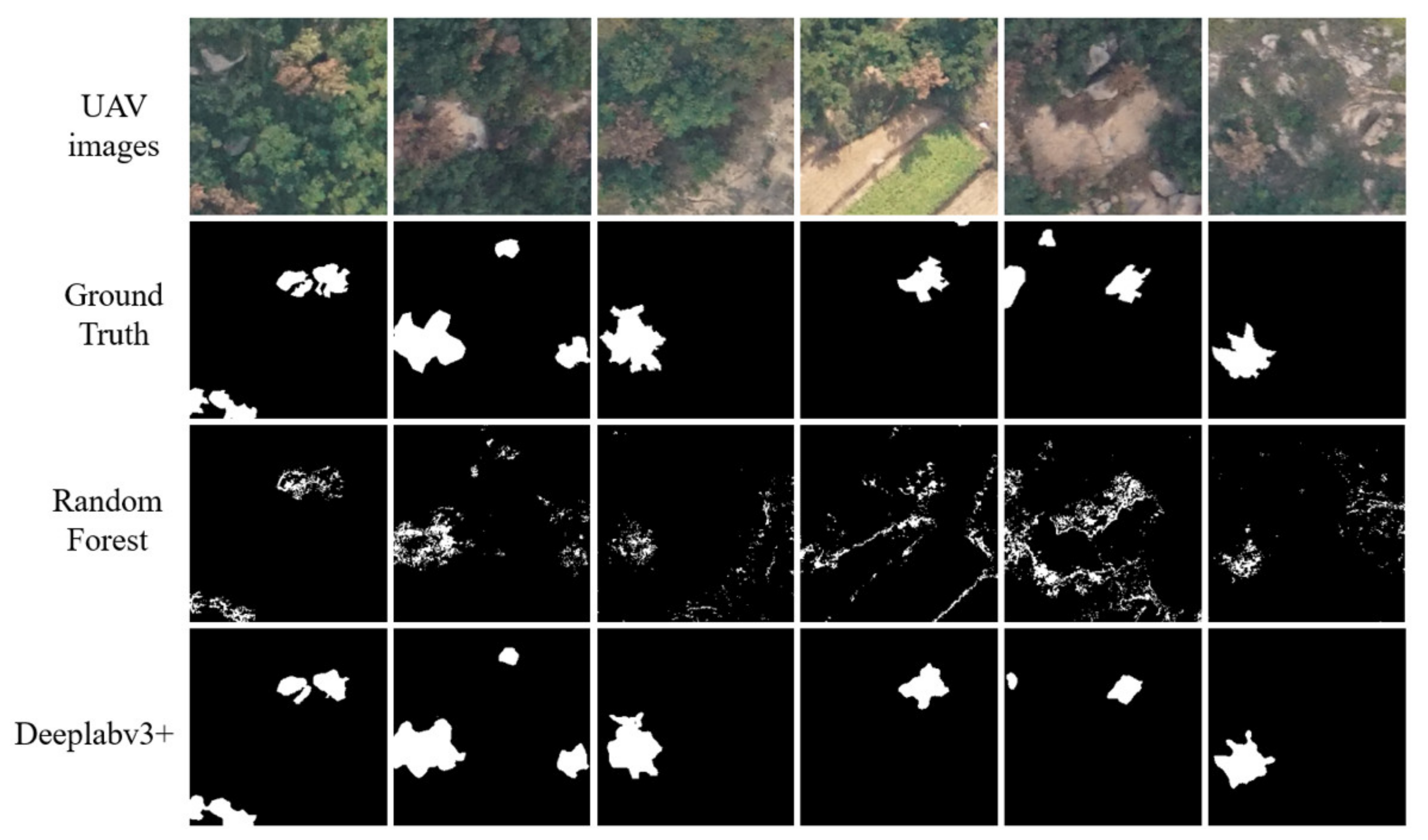
Performance of DL in remote sensing classification has been widely validated, and most studies demonstrated a larger margin than traditional machine learning methods. Then, what are the benefits of deep learning methods against traditional approaches in identification of wilt in pines? Here, we trained a widely used traditional machine learning method, Random Forest (RF), with the training dataset; the testing example is presented in Figure 7. As for the parameters of RF, the number of trees in the forest is 100, and the maximum depth of the tree is 5.
As indicated in Figure 7, the results of RF presented a heavy salt and pepper noise. RF can recognize most of the PWD pixels when the spectral reflectance difference between background and wilt pines is notable (e.g., in the first image); but, the result is quite poor when objects own similar spectral reflectance, such as bare soil and rock, as demonstrated in the fourth, fifth, and last image. The IoU and F1 of the RF method are 0.203, 0.337 respectively, which are lower than the best model Deeplabv3+, with 0.711 and 0.826. The best model presented in this study performed much better than the traditional machine learning method for wilt pine segmentations. In order to gain more accurate results, users should adopt the DL models presented in this study to replace traditional methods. Here, to increase availability in practice, the implemental codes and trained models are directly available at: https://github.com/xialang2012/PWD/tree/master (accessed 3 September 2021).

6. Conclusions

We used UAV images and annotation labels to evaluate high-performance DL segmentation models for identifying PWD-infected pines. A total of 7586 images from four areas were collected by a camera mounted on a fixed-wing UAV, and 45 images covering the main PWD areas were selected for evaluation. In the 45 images, 2352 infected pines were manually annotated. Validating the annotations based on ground survey data confirmed accurate and reliable labeling, with a mean accuracy of 97%.
Evaluating two common loss functions for training the models indicated that focal loss was more suitable than Dice loss for segmenting PWD-infected pines in UAV images. In fact, focal loss led to higher accuracy and finer boundaries than Dice loss, as the mean IoU indicated, which increased from 0.656 with Dice loss to 0.701 with focal loss. DeepLabv3+ achieved the highest IoU and F1 score of 0.720 and 0.832, respectively, indicating that the ASPP module encoded multiscale context information, and the encoder–decoder architecture to recover location/spatial information provided the highest performance for segmenting infected pines. The segmentation accuracy was sensitive to the backbone in the model, but the segmentation accuracy did not notably improve as the depth of the backbone increased. The results demonstrated that ResNet34 or ResNet50 was the appropriate backbone for most segmentation models.

Author Contributions

Data curation, L.X., R.Z., L.C., L.L., T.Y., Y.W., C.D. and C.X.; formal analysis, L.X.; funding acquisition, R.Z.; investigation, L.X., L.L. and T.Y.; methodology, L.X., R.Z., L.C. and L.L.; validation, C.D. and C.X.; writing—original draft, L.X., R.Z., L.C., T.Y. and Y.W.; writing—review and editing, L.X., R.Z., L.C. and C.D. All authors have read and agreed to the published version of the manuscript.

Funding

This work was support by the National Natural Science Foundation of China (32071907), BAAFS’ Innovation Ability Construction Program 2020 (KJCX20200206), and Outstanding Scientist Cultivation Project of Beijing Academy of Agriculture and Forestry Sciences (Grant No. JKZX201903).

Institutional Review Board Statement

Not applicable.

Informed Consent Statement

Not applicable.

Data Availability Statement

Not applicable.

Acknowledgments

We thank the Landscape and Forestry Bureau of Qindao for supporting the collection of UAV data.

Conflicts of Interest

The authors declare no conflict of interest. The funders had no role in the design of the study, in the collection, analyses, or interpretation of data, in the writing of the manuscript, or in the decision to publish the results.

References

  1. Proença, D.; Grass, G.; Morais, P.V. Understanding pine wilt disease: Roles of the pine endophytic bacteria and of the bacteria carried by the disease-causing pinewood nematode. MicrobiologyOpen 2016, 6, e00415. [Google Scholar] [CrossRef]
  2. Tang, X.; Yuan, Y.; Li, X.; Zhang, J. Maximum Entropy Modeling to Predict the Impact of Climate Change on Pine Wilt Disease in China. Front. Plant Sci. 2021, 12, 764. [Google Scholar] [CrossRef]
  3. Ding, X.; Wang, Q.; Guo, Y.; Li, Y.; Lin, S.; Zeng, Q.; Sun, F.; Li, D.-W.; Ye, J. Copy Number Variations of Glycoside Hydrolase 45 Genes in Bursaphelenchus xylophilus and Their Impact on the Pathogenesis of Pine Wilt Disease. Forests 2021, 12, 275. [Google Scholar] [CrossRef]
  4. Kim, N.; Jeon, H.W.; Mannaa, M.; Jeong, S.I.; Kim, J.; Kim, J.; Lee, C.; Park, A.R.; Kim, J.C.; Seo, Y.S. Induction of resistance against pine wilt disease caused by Bursaphelenchus xylophilus using selected pine endophytic bacteria. Plant Pathol. 2019, 68, 434–444. [Google Scholar] [CrossRef]
  5. Guo, D.S.; Zhao, B.G.; Gao, R. Experiments on the relationship between the bacterium isolate B619 and the pine wilt disease by using Calli of Pinus thunbergii. J. Nanjing For. Univ. 2001, 5, 71–74. [Google Scholar]
  6. Hirata, A.; Nakamura, K.; Nakao, K.; Kominami, Y.; Tanaka, N.; Ohashi, H.; Takano, K.; Takeuchi, W.; Matsui, T. Potential distribution of pine wilt disease under future climate change scenarios. PLoS ONE 2017, 12, e0182837. [Google Scholar] [CrossRef] [PubMed] [Green Version]
  7. National Forestry and Grassland Administration. Available online: http://www.forestry.gov.cn/main/5462/20210521/114505021470794.html (accessed on 21 May 2021).
  8. Firmino, P.N.; Calvão, T.; Ayres, M.P.; Pimentel, C. Monochamus galloprovincialis and Bursaphelenchus xylophilus life history in an area severely affected by pine wilt disease: Implications for forest management. For. Ecol. Manag. 2017, 389, 105–115. [Google Scholar] [CrossRef]
  9. Yoshimura, A.; Kawasaki, K.; Takasu, F.; Togashi, K.; Futai, K.; Shigesada, N. Modeling the spread of pine wilt disease caused by nematodes with pine sawyers as vector. Ecology 1999, 80, 1691–1702. [Google Scholar] [CrossRef]
  10. Wu, B.; Liang, A.; Zhang, H.; Zhu, T.; Zou, Z.; Yang, D.; Tang, W.; Li, J.; Su, J. Application of conventional UAV-based high-throughput object detection to the early diagnosis of pine wilt disease by deep learning. For. Ecol. Manag. 2021, 486, 118986. [Google Scholar] [CrossRef]
  11. Zhang, S.; Huang, J.; Hanan, J.; Qin, L. A hyperspectral GA-PLSR model for prediction of pine wilt disease. Multimed. Tools Appl. 2020, 79, 16645–16661. [Google Scholar] [CrossRef]
  12. Wu, W.; Zhang, Z.; Zheng, L.; Han, C.; Wang, X.; Xu, J.; Wang, X. Research Progress on the Early Monitoring of Pine Wilt Disease Using Hyperspectral Techniques. Sensors 2020, 20, 3729. [Google Scholar] [CrossRef] [PubMed]
  13. Zhou, X.; Liao, L.; Cheng, D.; Chen, X.; Huang, Q. Extraction of the Individual Tree Infected by Pine Wilt Disease Using Unmanned Aerial Vehicle Optical Imagery. Int. Arch. Photogramm. Remote. Sens. Spat. Inf. Sci. 2020, 43, 247–252. [Google Scholar] [CrossRef]
  14. Zhang, B.; Ye, H.; Lu, W.; Huang, W.; Wu, B.; Hao, Z.; Sun, H. A Spatiotemporal Change Detection Method for Monitoring Pine Wilt Disease in a Complex Landscape Using High-Resolution Remote Sensing Imagery. Remote. Sens. 2021, 13, 2083. [Google Scholar] [CrossRef]
  15. Zhang, R.; Xia, L.; Chen, L.; Xie, C.; Chen, M.; Wang, W. Recognition of wilt wood caused by pine wilt nematode based on U-Net network and unmanned aerial vehicle images. Trans. Chin. Soc. Agricult. Eng. 2020, 36, 61–68. [Google Scholar]
  16. White, J.C.; Wulder, M.A.; Brooks, D.; Reich, R.; Wheate, R.D. Detection of red attack stage mountain pine beetle infestation with high spatial resolution satellite imagery. Remote. Sens. Environ. 2005, 96, 340–351. [Google Scholar] [CrossRef]
  17. Hicke, J.A.; Logan, J. Mapping whitebark pine mortality caused by a mountain pine beetle outbreak with high spatial resolution satellite imagery. Int. J. Remote. Sens. 2009, 30, 4427–4441. [Google Scholar] [CrossRef]
  18. Kelcey, J.; Lucieer, A. Sensor Correction of a 6-Band Multispectral Imaging Sensor for UAV Remote Sensing. Remote. Sens. 2012, 4, 1462–1493. [Google Scholar] [CrossRef] [Green Version]
  19. Iordache, M.-D.; Mantas, V.; Baltazar, E.; Pauly, K.; Lewyckyj, N. A Machine Learning Approach to Detecting Pine Wilt Disease Using Airborne Spectral Imagery. Remote. Sens. 2020, 12, 2280. [Google Scholar] [CrossRef]
  20. Syifa, M.; Park, S.-J.; Lee, C.-W. Detection of the Pine Wilt Disease Tree Candidates for Drone Remote Sensing Using Artificial Intelligence Techniques. Engineering 2020, 6, 919–926. [Google Scholar] [CrossRef]
  21. Chollet, F. Xception: Deep learning with depthwise separable convolutions. In Proceedings of the IEEE Conference on Computer Vision and Pattern Recognition, Honolulu, HI, USA, 21–26 July 2017. [Google Scholar]
  22. He, K.; Zhang, X.; Ren, S.; Sun, J. Deep residual learning for image recognition. In Proceedings of the IEEE Conference on Computer Vision and Pattern Recognition, Las Vegas, NV, USA, 27–30 June 2016; pp. 770–778. [Google Scholar]
  23. Huang, G.; Liu, Z.; Van Der Maaten, L.; Weinberger, K.Q. Densely connected convolutional networks. In Proceedings of the IEEE Conference on Computer Vision and Pattern Recognition, Honolulu, HI, USA, 21–26 July 2017; pp. 4700–4708. [Google Scholar]
  24. Simonyan, K.; Zisserman, A. Very deep convolutional networks for large-scale image recognition. arXiv 2014, arXiv:1409.1556. [Google Scholar]
  25. He, K.; Gkioxari, G.; Dollár, P.; Girshick, R. Mask R-CNN. In Proceedings of the IEEE International Conference on Computer Vision, Venice, Italy, 22–29 October 2017; pp. 2961–2969. [Google Scholar]
  26. Hu, G.; Zhu, Y.; Wan, M.; Bao, W.; Zhang, Y.; Liang, D.; Yin, C. Detection of diseased pine trees in unmanned aerial vehicle images by using deep convolutional neural networks. Geocarto Int. 2021, 1–20. [Google Scholar] [CrossRef]
  27. Deng, X.; Tong, Z.; Lan, Y.; Huang, Z. Detection and Location of Dead Trees with Pine Wilt Disease Based on Deep Learning and UAV Remote Sensing. AgriEngineering 2020, 2, 19. [Google Scholar] [CrossRef]
  28. Tao, H.; Li, C.; Zhao, D.; Deng, S.; Hu, H.; Xu, X.; Jing, W. Deep learning-based dead pine tree detection from unmanned aerial vehicle images. Int. J. Remote. Sens. 2020, 41, 8238–8255. [Google Scholar] [CrossRef]
  29. Yu, R.; Luo, Y.; Zhou, Q.; Zhang, X.; Wu, D.; Ren, L. Early detection of pine wilt disease using deep learning algorithms and UAV-based multispectral imagery. For. Ecol. Manag. 2021, 497, 119493. [Google Scholar] [CrossRef]
  30. Qin, J.; Wang, B.; Wu, Y.; Lu, Q.; Zhu, H. Identifying Pine Wood Nematode Disease Using UAV Images and Deep Learning Algorithms. Remote. Sens. 2021, 13, 162. [Google Scholar] [CrossRef]
  31. Evan, S.; Trevor, D. Fully convolutional networks for semantic segmentation. In Proceedings of the IEEE Conference on Computer Vision and Pattern Recognition, Boston, MA, USA, 7–12 June 2015; pp. 3431–3440. [Google Scholar]
  32. Zhao, H.; Shi, J.; Qi, X.; Wang, X.; Jia, J. Pyramid scene parsing network. In Proceedings of the IEEE Conference on Computer Vision and Pattern Recognition, Honolulu, HI, USA, 21–26 July 2017; pp. 2881–2890. [Google Scholar]
  33. Ronneberger, O.; Philipp, F.; Thomas, B. U-net: Convolutional networks for biomedical image segmentation. In International Conference on Medical Image Computing and Computer-Assisted Intervention; Springer: Cham, Switzerland, 2015; pp. 234–241. [Google Scholar]
  34. Badrinarayanan, V.; Kendall, A.; Cipolla, R. SegNet: A Deep Convolutional Encoder-Decoder Architecture for Image Segmentation. IEEE Trans. Pattern Anal. Mach. Intell. 2017, 39, 2481–2495. [Google Scholar] [CrossRef]
  35. Chen, L.C.; Papandreou, G.; Schroff, F.; Adam, H. Rethinking atrous convolution for semantic image segmentation. arXiv 2017, arXiv:1706.05587. [Google Scholar]
  36. Yang, M.; Yu, K.; Zhang, C.; Li, Z.; Yang, K. Denseaspp for semantic segmentation in street scenes. In Proceedings of the IEEE Conference on Computer Vision and Pattern Recognition, Salt Lake City, UT, USA, 18–23 June 2018; pp. 3684–3692. [Google Scholar]
  37. Chen, L.C.; Zhu, Y.; Papandreou, G.; Schroff, F.; Adam, H. Encoder-decoder with atrous separable convolution for semantic image segmentation. In Proceedings of the European Conference on Computer Vision (ECCV), Munich, Germany, 8–14 September 2018; pp. 801–818. [Google Scholar]
  38. Fu, J.; Liu, J.; Tian, H.; Li, Y.; Bao, Y.; Fang, Z.; Lu, H. Dual attention network for scene seg-mentation. In Proceedings of the IEEE/CVF Conference on Computer Vision and Pattern Recognition, Long Beach, CA, USA, 15–20 June 2019; pp. 3146–3154. [Google Scholar]
  39. Yuan, Y.; Huang, L.; Guo, J.; Zhang, C.; Chen, X.; Wang, J. Ocnet: Object context network for scene parsing. arXiv 2018, arXiv:1809.00916. [Google Scholar]
  40. Huang, Q.; Sun, J.; Ding, H.; Wang, X.; Wang, G. Robust liver vessel extraction using 3D U-Net with variant dice loss function. Comput. Biol. Med. 2018, 101, 153–162. [Google Scholar] [CrossRef]
  41. Lin, T.Y.; Goyal, P.; Girshick, R.; He, K.; Dollár, P. Focal loss for dense object detection. In Proceedings of the IEEE International Conference on Computer Vision, Venice, Italy, 22–29 October 2017; pp. 2980–2988. [Google Scholar]
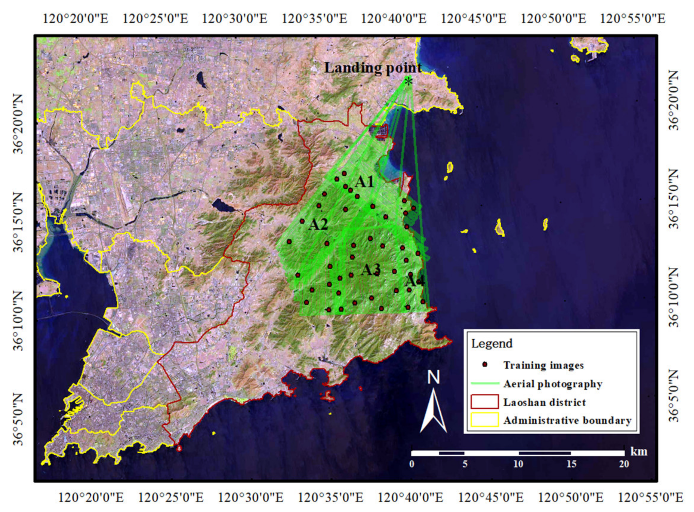
Figure 1. Study area.
Remotesensing 13 03594 g001
Figure 2. Researchers conducting field survey of PWD-infected pines (first row) and images of infected pines (second to fifth rows).
Remotesensing 13 03594 g002
Figure 3. Annotation results of infected pines, the full UAV image and the result of annotation (first-row), and the clipped samples (other rows).
Remotesensing 13 03594 g003
Figure 4. Segmentation results of models using Dice loss.
Remotesensing 13 03594 g004
Figure 5. Segmentation results of models using focal loss.
Remotesensing 13 03594 g005
Figure 6. Segmenting results of DeepLabv3 and DeepLabv3+ using the ResNet34 backbone.
Remotesensing 13 03594 g006
Figure 7. Comparison between the best DL model, Deeplabv3+, and the traditional machine learning method RF.
Remotesensing 13 03594 g007
Table 1. Models evaluated in this study.
ModelSourceNo. ParametersBackboneFeatures
FCNLong et al., 201515,305,667XceptionMilestone segmentation model
PSPNetZhao et al., 201748,755,113ResNetMultiscale feature fusion using pyramid pooling or
symmetric encoder–decoder
U-NetRonneberger et al., 201526,355,169ResNet
SegNetBadrinarayanan et al., 201516,310,273VGG16
DeepLabv3Chen et al., 201741,806,505ResNetDilated convolution
DenseASPPYang et al., 201827,161,537ResNet
DeepLabv3+Chen et al., 201874,982,817ResNet
DANetFu et al., 201949,607,725ResNetAttention network
OCNetYuan et al., 201836,040,105ResNet
Table 2. Performance of different models using Dice loss.
ModelIoUF1 ScorePrecisionRecall
FCN0.6720.7980.8050.791
PSPNet0.6490.7810.7530.811
U-Net0.6670.7980.7670.831
SegNet0.6520.7780.7640.793
DeepLabv30.6510.7780.8060.752
DeepLabv3+0.6820.8060.7910.822
DenseASPP0.6760.7980.8060.790
DANet0.6340.7710.7690.773
OCNet0.6210.7640.7370.794
Mean0.6560.7860.7780.795
Table 3. Performance of different models using focal loss.
ModelIoUF1 ScorePrecisionRecall
FCN0.6790.8030.8100.797
PSPNet0.7070.8210.8440.799
U-Net0.7080.8190.8240.815
SegNet0.6980.8090.8140.805
DeepLabv30.6990.8190.8630.780
DeepLabv3+0.7200.8320.8380.826
DenseASPP0.7170.8310.8330.829
DANet0.6750.8000.8000.800
OCNet0.7080.8250.8380.813
Mean0.7010.8180.8290.807
Improvement over models trained with Dice loss (%)6.864.086.561.51
Table 4. Model performance for different backbones.
ModelBackboneIoUF1PrecisionRecall
PSPNetResNet340.7200.8280.8470.811
ResNet500.7070.8210.8440.799
ResNet1010.7060.8210.8560.789
ResNet1520.7100.8230.8200.825
DeepLabv3+ResNet340.7200.8320.8310.832
ResNet500.7200.8320.8380.826
ResNet1010.7180.8310.8460.817
ResNet1520.7140.8300.8240.835
OCNetResNet340.7180.8320.8410.823
ResNet500.7080.8250.8380.813
ResNet1010.7010.8070.8340.807
ResNet1520.6910.8120.8370.789
Table 5. Performance of DeepLabv3 and DeepLabv3+ for different backbones.
ModelBackboneIoUF1 scorePrecisionRecall
DeepLabv3ResNet340.7110.8260.8260.825
ResNet500.6990.8190.8630.780
ResNet1010.7010.8190.8440.795
ResNet1520.7060.8190.8200.819
DeepLabv3+ResNet340.7200.8320.8310.832
ResNet500.7200.8320.8380.826
ResNet1010.7180.8310.8460.817
ResNet1520.7140.8300.8240.835
Publisher’s Note: MDPI stays neutral with regard to jurisdictional claims in published maps and institutional affiliations.