
Assessing Forest Type and Tree Species Classification Using Sentinel-1 C-Band SAR Data in Southern Sweden


Abstract
:1. Introduction
2. Materials and Methods
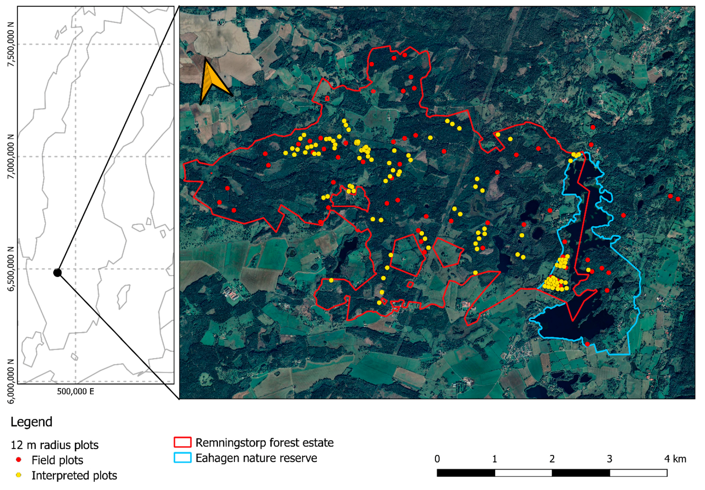
2.1. Study Areas
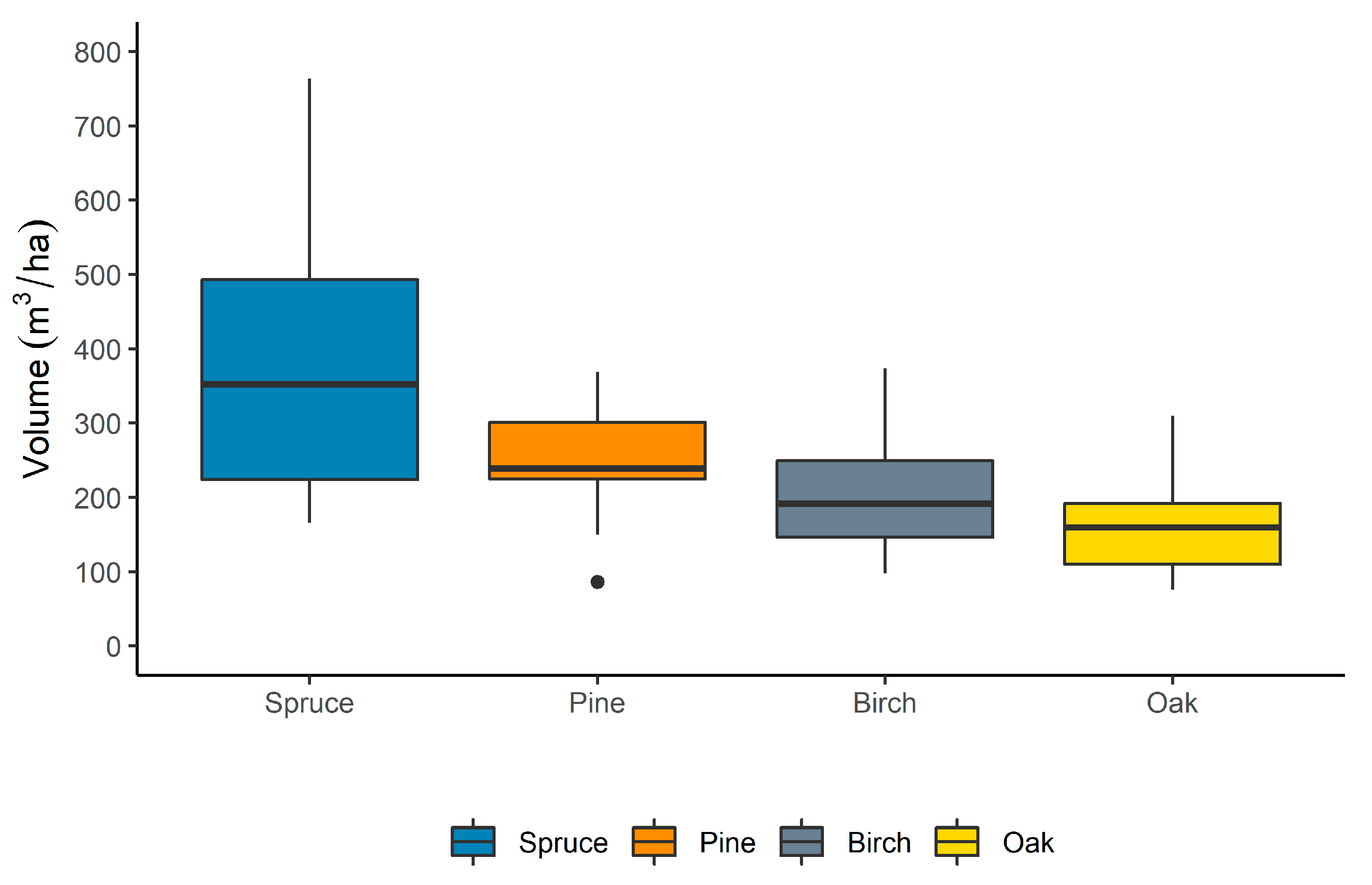
2.2. Field Data
2.3. Satellite Data
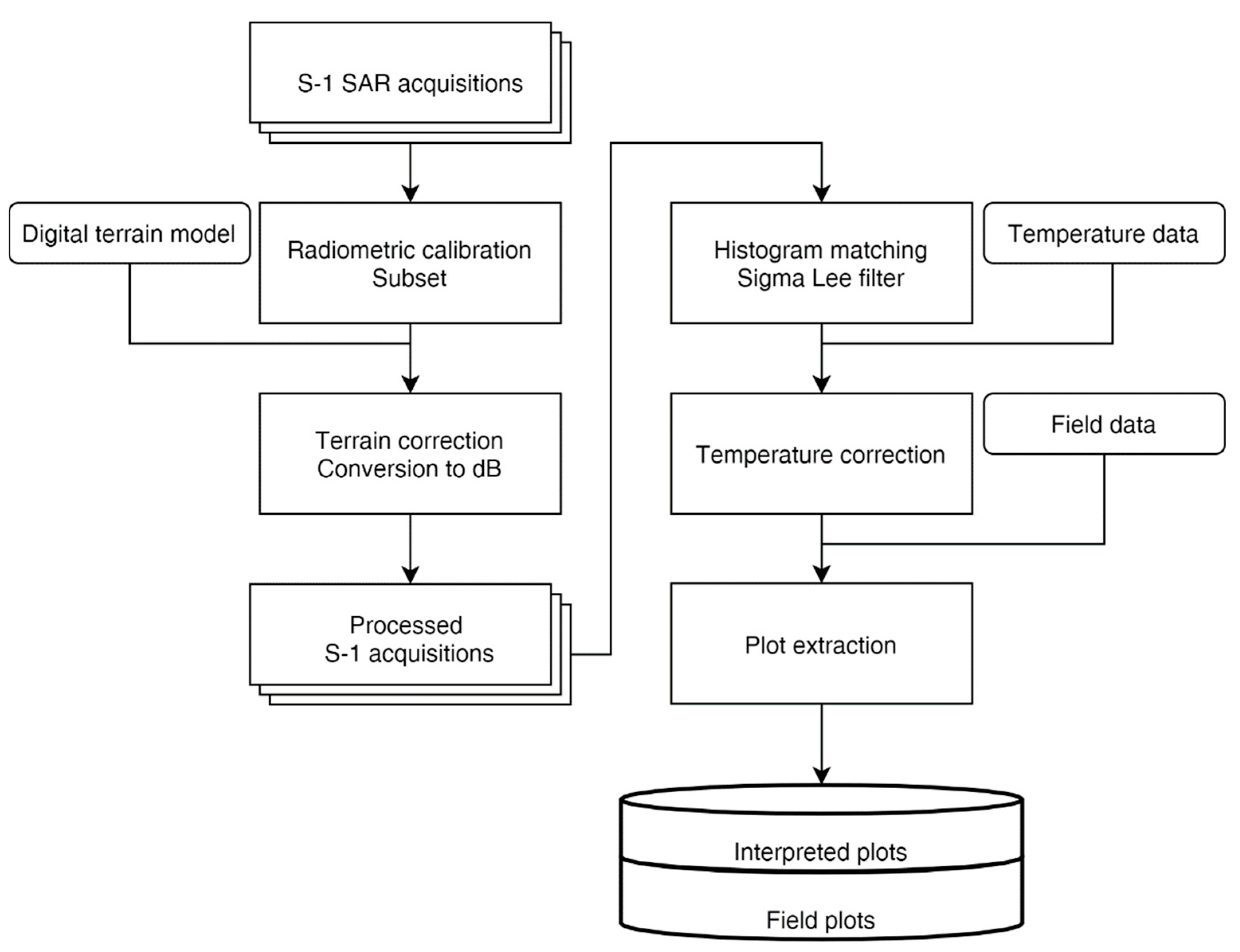
2.4. Pre-Processing of Satellite Images
2.5. Classification and Validation
2.6. Seasonality
3. Results
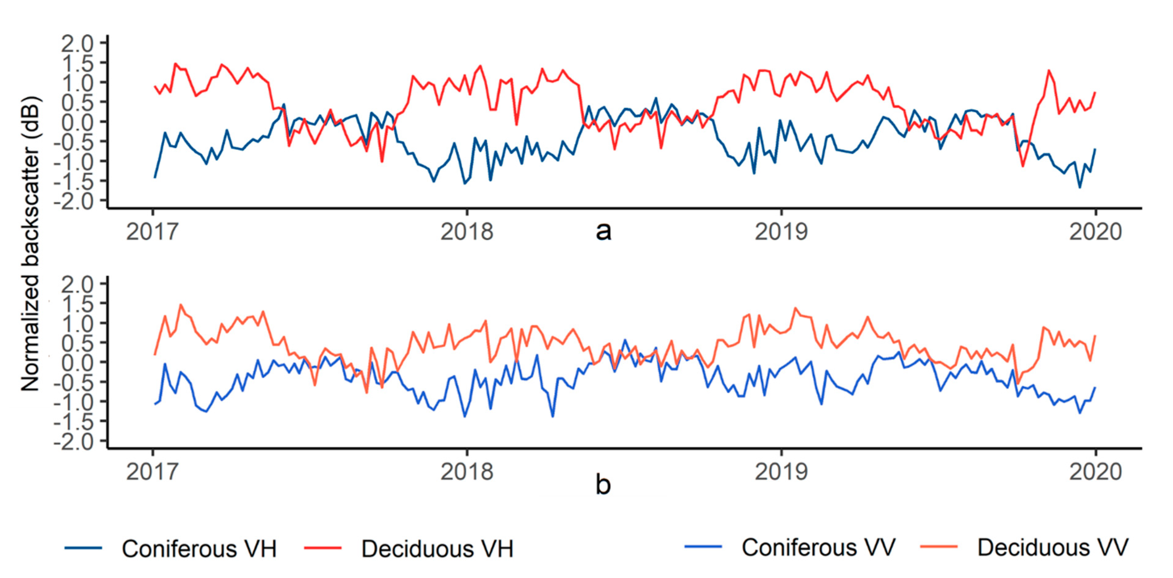
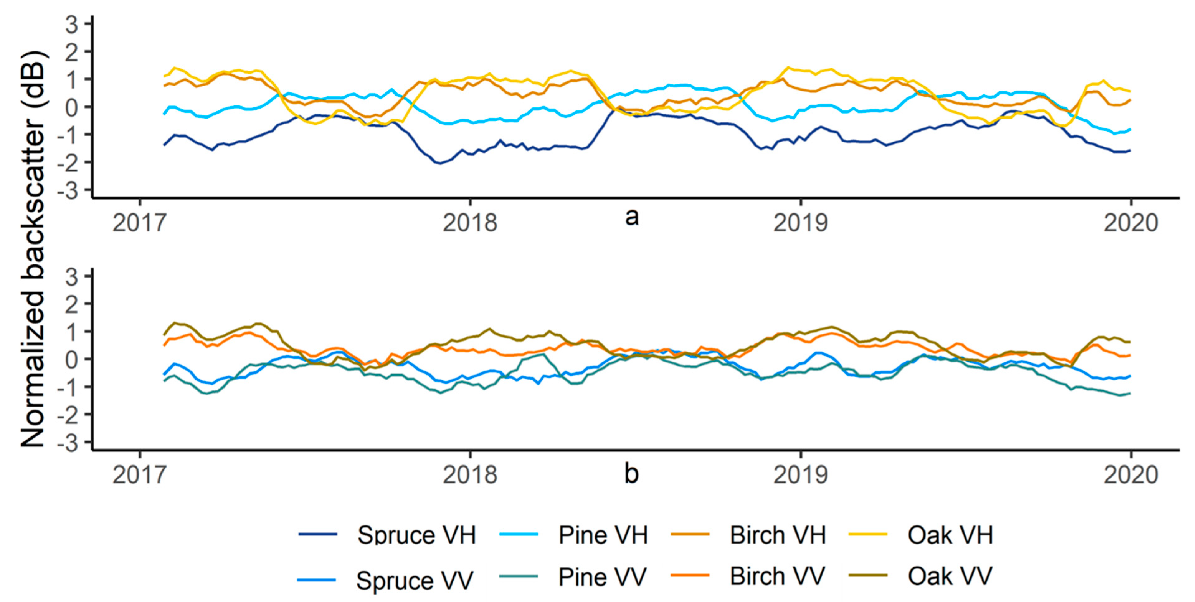
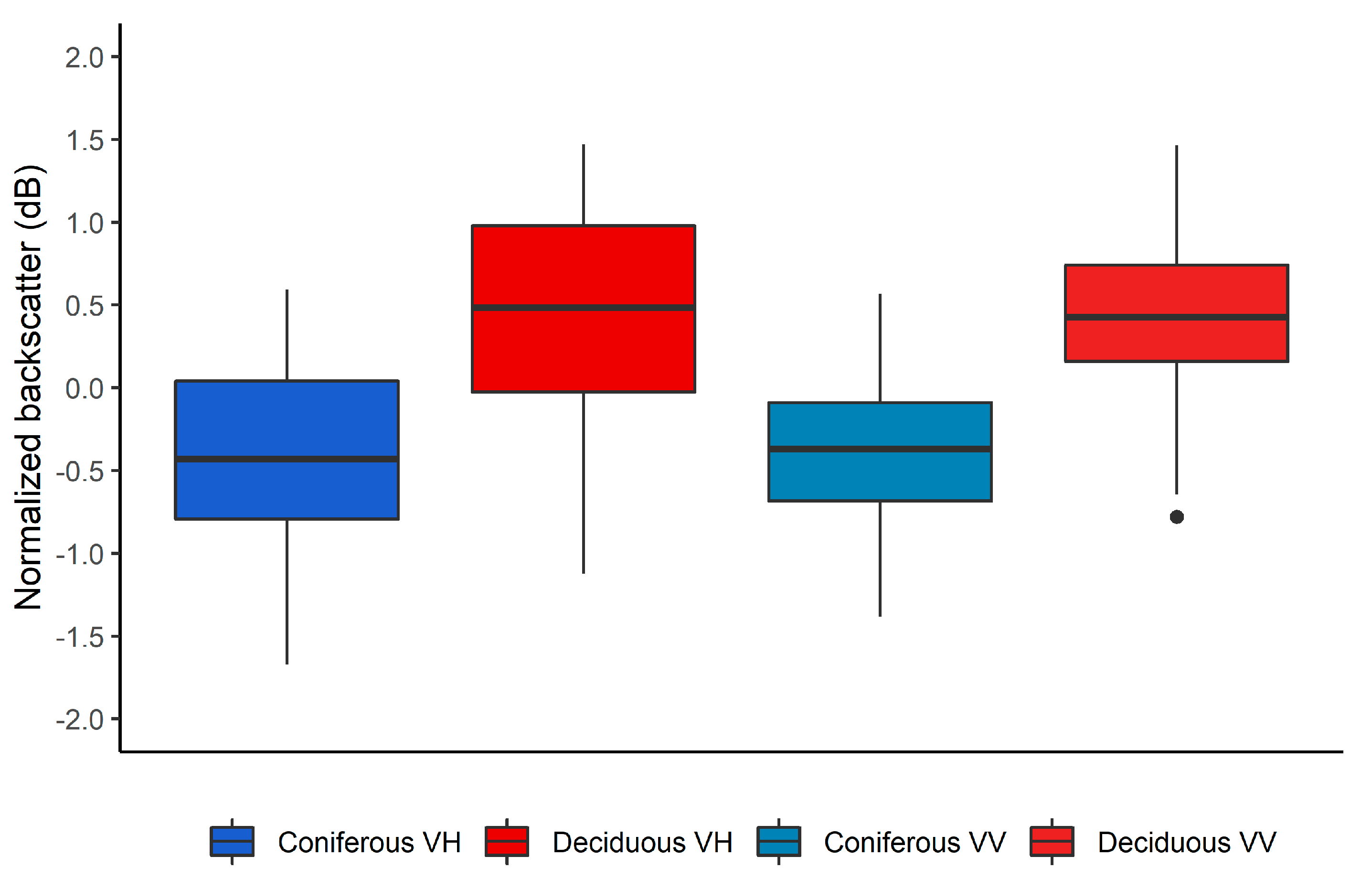
3.1. Backscatter Trend
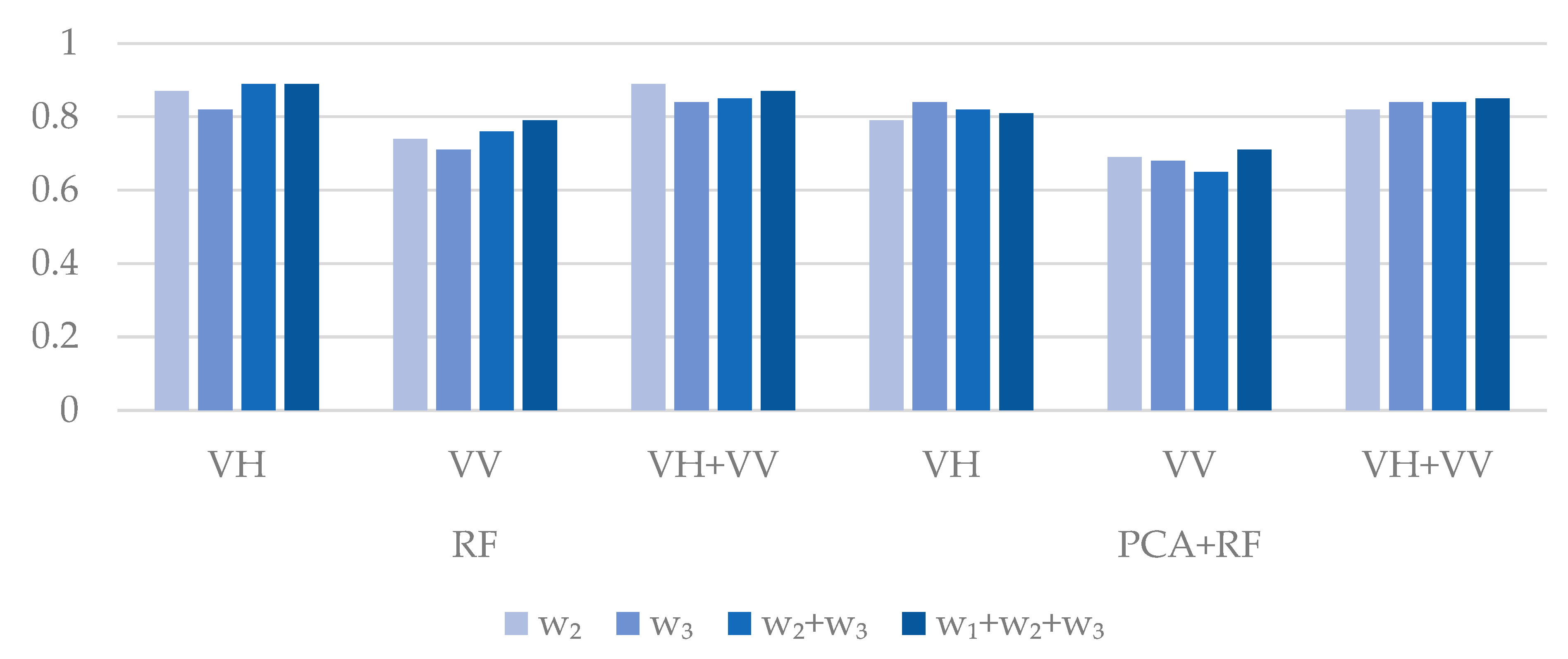
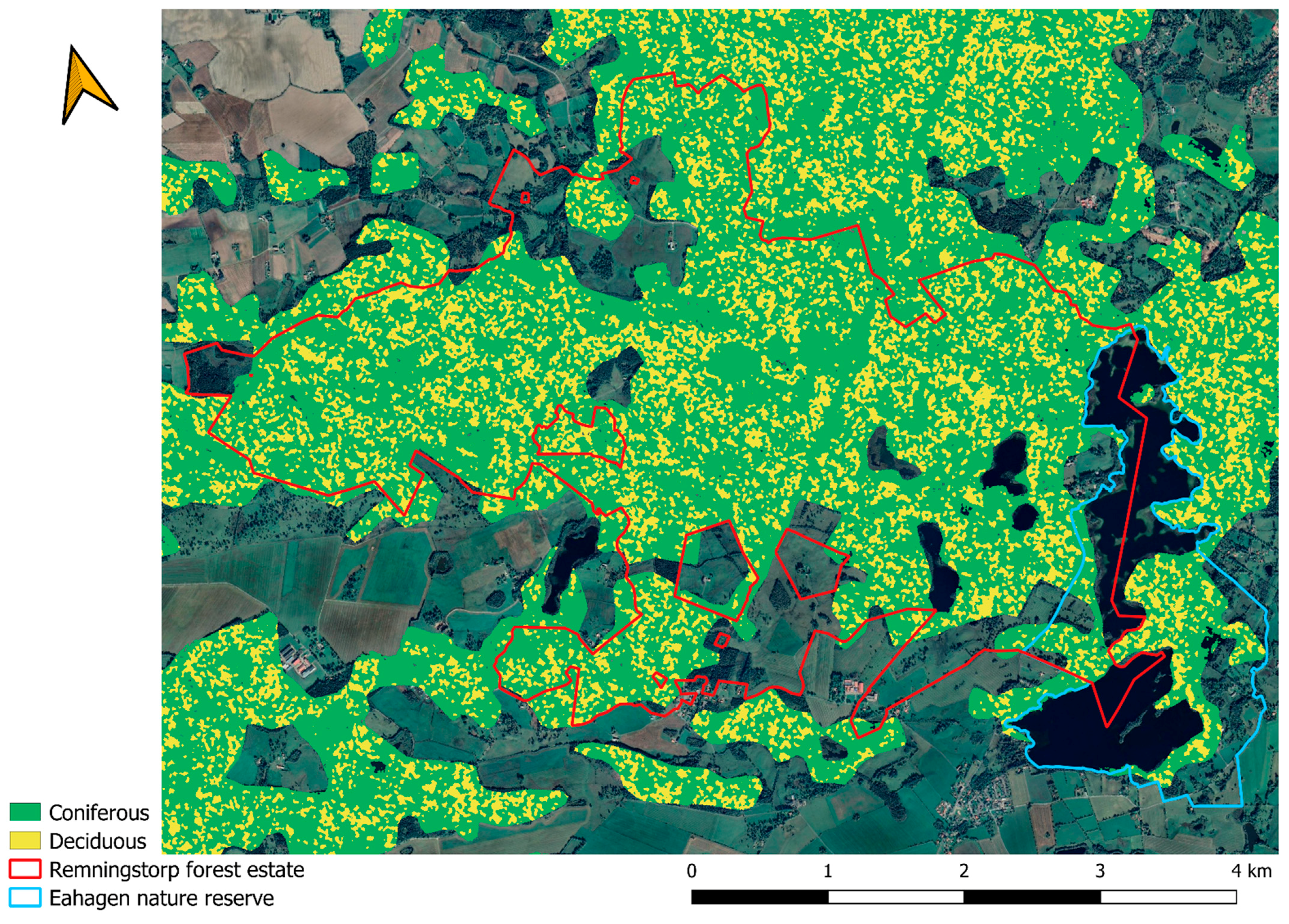
3.2. Forest Type Classification
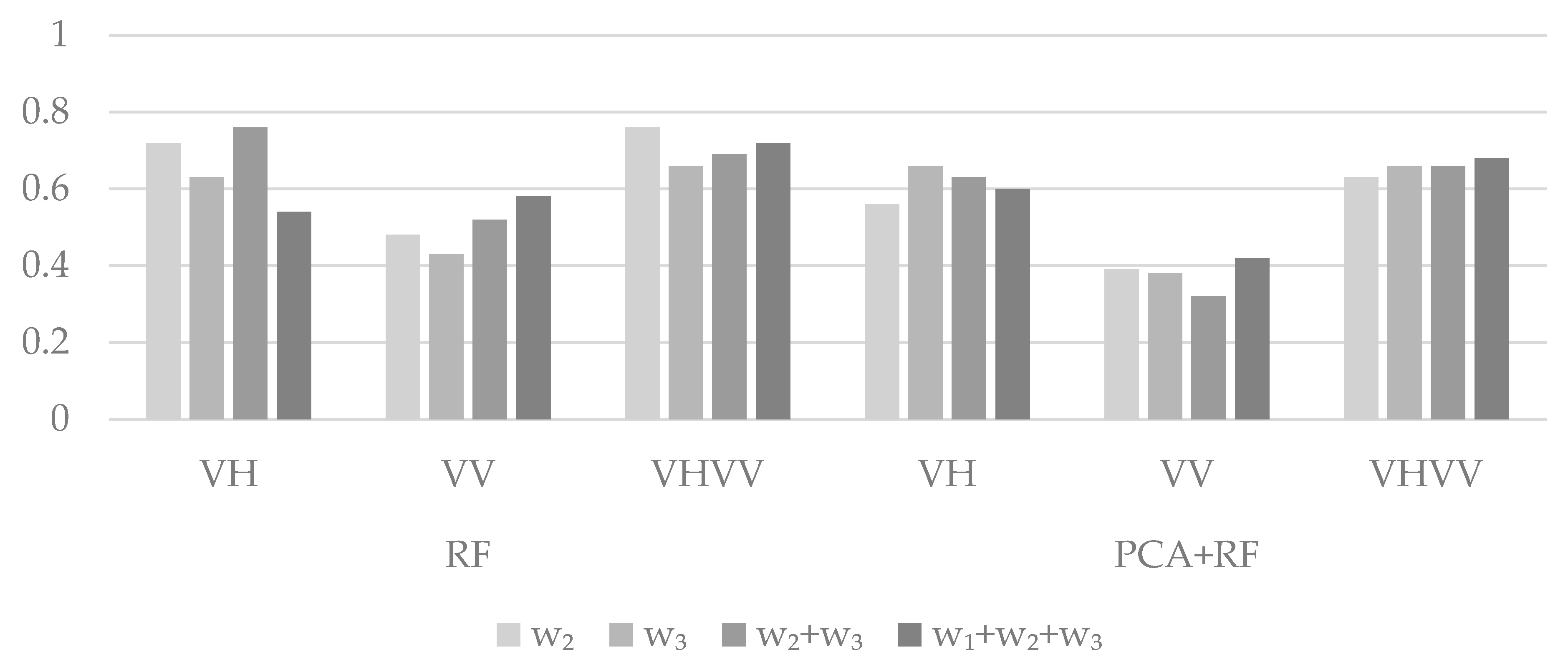
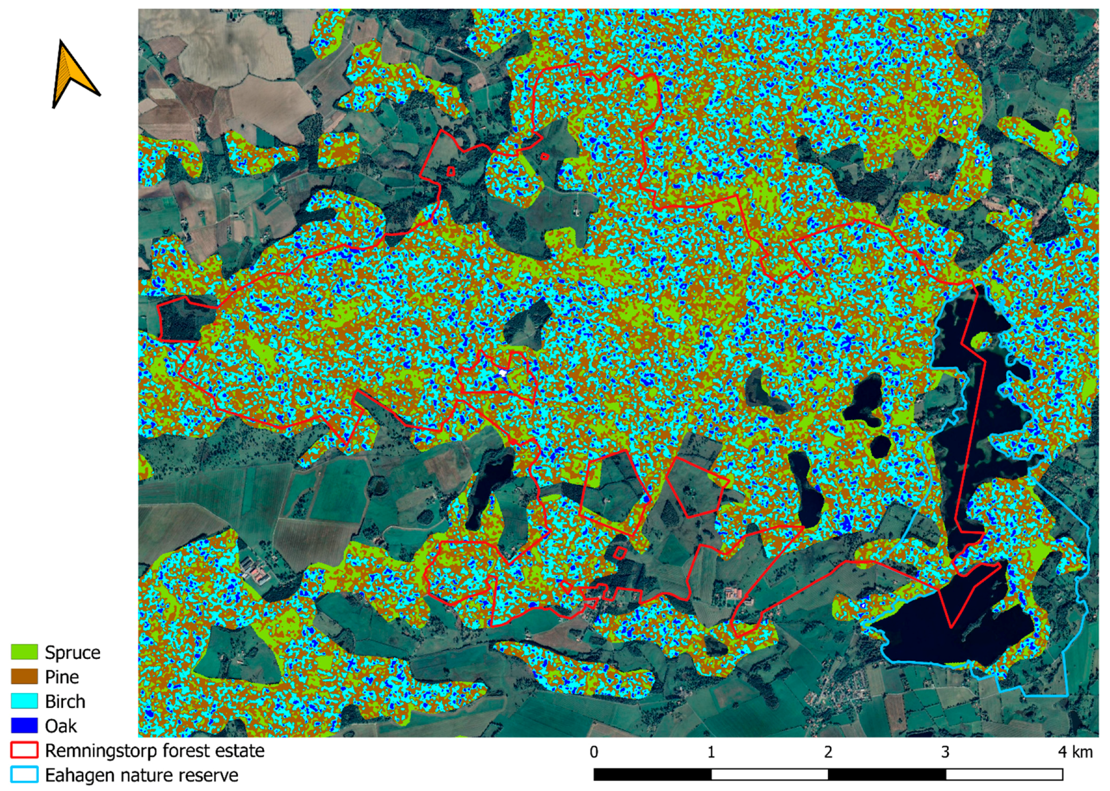
3.3. Species Classification
3.4. Seasonality
4. Discussion
5. Conclusions
- The proposed approach showed good results with the FTY classification overall accuracy reaching 94%. We obtained high values for both producer’s and user’s accuracy, ranging between 84 and 100%, which was convincing also compared to similar studies [28,29,55]. Moreover, the RF model for the classification achieved high values also in Cohen’s K, indicating a high degree of agreement between field and predicted values. The accuracy results indicate that this method is suitable for the creation and use of FTY maps (Figure 6) [12,56].
- The use of multiple winter seasons delivered better accuracies compared to the use of single winter seasons. The VH polarization contained most of the information and by using the VH + VV combination, the results improved slightly. The differences between forest types were biggest during the winters and by using winter images the results were almost as high as using all year round images.
- The use of PCA generally improved the classifications of both forest type and tree species, although this was not the case when using only winter images.
Author Contributions
Funding
Institutional Review Board Statement
Informed Consent Statement
Data Availability Statement
Conflicts of Interest
Appendix A

| Confusion Matrix | |||||
|---|---|---|---|---|---|
| Reference | Classification | PA | OA | K | |
| Coniferous | Deciduous | ||||
| Coniferous | 38 | 3 | 0.93 | 0.94 | 0.86 |
| Deciduous | 1 | 20 | 0.95 | ||
| UA | 0.97 | 0.87 | |||
| Confusion Matrix | |||||
|---|---|---|---|---|---|
| Reference | Classification | PA | OA | K | |
| Coniferous | Deciduous | ||||
| Coniferous | 27 | 14 | 0.66 | 0.73 | 0.46 |
| Deciduous | 3 | 18 | 0.86 | ||
| UA | 0.90 | 0.56 | |||
| Confusion Matrix | |||||
|---|---|---|---|---|---|
| Reference | Classification | PA | OA | K | |
| Coniferous | Deciduous | ||||
| Coniferous | 36 | 5 | 0.88 | 0.89 | 0.76 |
| Deciduous | 2 | 19 | 0.90 | ||
| UA | 0.95 | 0.79 | |||
| Confusion Matrix | |||||
|---|---|---|---|---|---|
| Reference | Classification | PA | OA | K | |
| Coniferous | Deciduous | ||||
| Coniferous | 36 | 5 | 0.88 | 0.92 | 0.83 |
| Deciduous | 0 | 21 | 1.00 | ||
| UA | 1.00 | 0.81 | |||
| Confusion Matrix | |||||
|---|---|---|---|---|---|
| Reference | Classification | PA | OA | K | |
| Coniferous | Deciduous | ||||
| Coniferous | 32 | 9 | 0.78 | 0.84 | 0.67 |
| Deciduous | 1 | 20 | 0.95 | ||
| UA | 0.97 | 0.69 | |||
| Confusion Matrix | |||||
|---|---|---|---|---|---|
| Reference | Classification | PA | OA | K | |
| Coniferous | Deciduous | ||||
| Coniferous | 37 | 4 | 0.90 | 0.94 | 0.86 |
| Deciduous | 0 | 21 | 1.00 | ||
| UA | 1.00 | 0.84 | |||
| Confusion Matrix | |||||||
|---|---|---|---|---|---|---|---|
| Reference | Classification | PA | OA | K | |||
| Birch | Oak | Pine | Spruce | ||||
| Birch | 1 | 7 | 0 | 0 | 0.13 | 0.55 | 0.39 |
| Oak | 0 | 11 | 1 | 1 | 0.85 | ||
| Pine | 2 | 0 | 11 | 0 | 0.85 | ||
| Spruce | 0 | 1 | 16 | 11 | 0.39 | ||
| UA | 0.33 | 0.58 | 0.39 | 0.92 | |||
| Confusion Matrix | |||||||
|---|---|---|---|---|---|---|---|
| Reference | Classification | PA | OA | K | |||
| Birch | Oak | Pine | Spruce | ||||
| Birch | 2 | 5 | 1 | 0 | 0.25 | 0.35 | 0.19 |
| Oak | 1 | 9 | 3 | 0 | 0.69 | ||
| Pine | 0 | 2 | 11 | 0 | 0.85 | ||
| Spruce | 2 | 4 | 22 | 0 | 0.00 | ||
| UA | 0.40 | 0.45 | 0.30 | - | |||
| Confusion Matrix | |||||||
|---|---|---|---|---|---|---|---|
| Reference | Classification | PA | OA | K | |||
| Birch | Oak | Pine | Spruce | ||||
| Birch | 1 | 7 | 0 | 0 | 0.13 | 0.50 | 0.35 |
| Oak | 0 | 11 | 2 | 0 | 0.85 | ||
| Pine | 0 | 1 | 12 | 0 | 0.92 | ||
| Spruce | 0 | 2 | 19 | 7 | 0.25 | ||
| UA | 1.00 | 0.52 | 0.36 | 1.00 | |||
| Confusion Matrix | |||||||
|---|---|---|---|---|---|---|---|
| Reference | Classification | PA | OA | K | |||
| Birch | Oak | Pine | Spruce | ||||
| Birch | 3 | 5 | 0 | 0 | 0.38 | 0.66 | 0.54 |
| Oak | 1 | 12 | 0 | 0 | 0.92 | ||
| Pine | 3 | 0 | 9 | 1 | 0.69 | ||
| Spruce | 0 | 2 | 9 | 17 | 0.61 | ||
| UA | 0.43 | 0.63 | 0.50 | 0.94 | |||
| Confusion Matrix | |||||||
|---|---|---|---|---|---|---|---|
| Reference | Classification | PA | OA | K | |||
| Birch | Oak | Pine | Spruce | ||||
| Birch | 5 | 2 | 1 | 0 | 0.63 | 0.48 | 0.35 |
| Oak | 3 | 10 | 0 | 0 | 0.77 | ||
| Pine | 3 | 0 | 10 | 0 | 0.77 | ||
| Spruce | 7 | 3 | 13 | 5 | 0.18 | ||
| UA | 0.28 | 0.67 | 0.42 | 1.00 | |||
| Confusion Matrix | |||||||
|---|---|---|---|---|---|---|---|
| Reference | Classification | PA | OA | K | |||
| Birch | Oak | Pine | Spruce | ||||
| Birch | 4 | 4 | 0 | 0 | 0.50 | 0.53 | 0.39 |
| Oak | 2 | 11 | 0 | 0 | 0.85 | ||
| Pine | 1 | 0 | 10 | 2 | 0.77 | ||
| Spruce | 1 | 3 | 16 | 8 | 0.29 | ||
| UA | 0.50 | 0.61 | 0.38 | 0.80 | |||
| w2 | w3 | w2 + w3 | w1 + w2 + w3 | ||
|---|---|---|---|---|---|
| Coniferous | PA | 0.85 | 0.78 | 0.88 | 0.88 |
| UA | 0.95 | 0.94 | 0.95 | 0.95 | |
| Deciduous | PA | 0.90 | 0.90 | 0.90 | 0.90 |
| UA | 0.76 | 0.68 | 0.79 | 0.79 | |
| OA | 0.87 | 0.82 | 0.89 | 0.89 | |
| K | 0.72 | 0.63 | 0.76 | 0.76 |
| w2 | w3 | w2 + w3 | w1 + w2 + w3 | ||
|---|---|---|---|---|---|
| Coniferous | PA | 0.68 | 0.63 | 0.68 | 0.73 |
| UA | 0.90 | 0.90 | 0.93 | 0.94 | |
| Deciduous | PA | 0.86 | 0.86 | 0.90 | 0.90 |
| UA | 0.58 | 0.55 | 0.59 | 0.63 | |
| OA | 0.74 | 0.71 | 0.76 | 0.65 | |
| K | 0.48 | 0.43 | 0.52 | 0.32 |
| w2 | w3 | w2 + w3 | w1 + w2 + w3 | ||
|---|---|---|---|---|---|
| Coniferous | PA | 0.88 | 0.80 | 0.83 | 0.85 |
| UA | 0.95 | 0.94 | 0.94 | 0.95 | |
| Deciduous | PA | 0.90 | 0.90 | 0.90 | 0.90 |
| UA | 0.79 | 0.70 | 0.73 | 0.76 | |
| OA | 0.89 | 0.84 | 0.85 | 0.87 | |
| K | 0.76 | 0.66 | 0.69 | 0.72 |
| w2 | w3 | w2 + w3 | w1 + w2 + w3 | ||
|---|---|---|---|---|---|
| Coniferous | PA | 0.78 | 0.80 | 0.80 | 0.78 |
| UA | 0.89 | 0.94 | 0.92 | 0.91 | |
| Deciduous | PA | 0.81 | 0.90 | 0.86 | 0.86 |
| UA | 0.65 | 0.70 | 0.69 | 0.67 | |
| OA | 0.79 | 0.84 | 0.82 | 0.81 | |
| K | 0.56 | 0.66 | 0.63 | 0.60 |
| w2 | w3 | w2 + w3 | w1 + w2 + w3 | ||
|---|---|---|---|---|---|
| Coniferous | PA | 0.63 | 0.59 | 0.56 | 0.66 |
| UA | 0.87 | 0.89 | 0.85 | 0.87 | |
| Deciduous | PA | 0.81 | 0.86 | 0.81 | 0.81 |
| UA | 0.53 | 0.51 | 0.49 | 0.55 | |
| OA | 0.69 | 0.68 | 0.65 | 0.71 | |
| K | 0.39 | 0.38 | 0.32 | 0.42 |
| w2 | w3 | w2 + w3 | w1 + w2 + w3 | ||
|---|---|---|---|---|---|
| Coniferous | PA | 0.80 | 0.83 | 0.83 | 0.88 |
| UA | 0.92 | 0.92 | 0.92 | 0.90 | |
| Deciduous | PA | 0.86 | 0.86 | 0.86 | 0.81 |
| UA | 0.69 | 0.72 | 0.72 | 0.77 | |
| OA | 0.82 | 0.84 | 0.84 | 0.85 | |
| K | 0.63 | 0.66 | 0.66 | 0.55 |

References
- Ostrom, E. Understanding Institutional Diversity; Princeton University Press: Priceton, NJ, USA, 2009; ISBN 9781400831739. [Google Scholar]
- FAO. Global Forest Resources Assessment 2020: Main Report; FAO: Rome, Italy, 2020. [Google Scholar]
- Nemani, R.R.; Running, S.W. Satellite Monitoring of Global Land Cover Changes and their Impact on Climate. In Long-Term Climate Monitoring by the Global Climate Observing System; Springer: Dordrecht, The Netherlands, 1996; pp. 265–283. [Google Scholar]
- Innes, J.L.; Koch, B. Forest biodiversity and its assessment by remote sensing. Glob. Ecol. Biogeogr. 1998, 7, 397–419. [Google Scholar] [CrossRef]
- Lindenmayer, D.B.; Margules, C.R.; Botkin, D.B. Indicators of biodiversity for ecologically sustainable forest management. Conserv. Biol. 2000, 14, 941–950. [Google Scholar] [CrossRef]
- MacDicken, K.G. Global Forest Resources Assessment 2015: What, why and how? For. Ecol. Manag. 2015, 352, 3–8. [Google Scholar] [CrossRef] [Green Version]
- Gustafson, E.; Keene, R. Predicting Changes in Forest Composition and Dynamics—Landscape-Scale Process Models; U.S. Department of Agriculture, Forest Service, Climate Change Resource Center: Washington, DC, USA, 2014.
- Pettorelli, N.; Laurance, W.F.; O’Brien, T.G.; Wegmann, M.; Nagendra, H.; Turner, W. Satellite remote sensing for applied ecologists: Opportunities and challenges. J. Appl. Ecol. 2014, 51, 839–848. [Google Scholar] [CrossRef]
- Korpela, I. Individual tree measurements by means of digital aerial photogrammetry. Silva Fenn. Monogr. 2004, 3, 1–93. [Google Scholar]
- King, D.J. Airborne remote sensing in forestry: Sensors, analysis and applications. For. Chron. 2000, 76, 859–876. [Google Scholar] [CrossRef] [Green Version]
- Yu, X.; Hyyppä, J.; Karjalainen, M.; Nurminen, K.; Karila, K.; Vastaranta, M.; Kankare, V.; Kaartinen, H.; Holopainen, M.; Honkavaara, E.; et al. Comparison of laser and stereo optical, SAR and InSAR point clouds from air- and space-borne sources in the retrieval of forest inventory attributes. Remote Sens. 2015, 7, 15933–15954. [Google Scholar] [CrossRef] [Green Version]
- Fassnacht, F.E.; Latifi, H.; Stereńczak, K.; Modzelewska, A.; Lefsky, M.; Waser, L.T.; Straub, C.; Ghosh, A. Review of studies on tree species classification from remotely sensed data. Remote Sens. Environ. 2016, 186, 64–87. [Google Scholar] [CrossRef]
- Benallegue, M.; Taconet, O.; Vidal-Madjar, D.; Normand, M. The use of radar backscattering signals for measuring soil moisture and surface roughness. Remote Sens. Environ. 1995, 53, 61–68. [Google Scholar] [CrossRef]
- Kirscht, M.; Rinke, C. 3D reconstruction of buildings and vegetation from SAR images. In Proceedings of the IAPR Workshop on Machine Vision Applications, Chiba, Japan, 17–19 November 1998; pp. 228–231. [Google Scholar]
- Meyer, F. Spaceborne Synthetic Aperture Radar: Principles, Data Access, and Basic Processing Techniques. In The Synthetic Aperture Radar (SAR) Handbook: Comprehensive Methodologies for Forest Monitoring and Biomass Estimation; Flores, A., Herndon, K., Thapa, R., Cherrington, E., Eds.; NASA: Houston, TX, USA, 2019; pp. 21–40. [Google Scholar]
- Ningthoujam, R.K.; Tansey, K.; Balzter, H.; Morrison, K.; Johnson, S.C.M.; Gerard, F.; George, C.; Burbidge, G.; Doody, S.; Veck, N.; et al. Mapping forest cover and forest cover change with airborne S-band radar. Remote Sens. 2016, 8, 577. [Google Scholar] [CrossRef] [Green Version]
- Saatchi, S. SAR Methods for Mapping and Monitoring Forest Biomass. In The SAR Handbook. Comprehensive Methodologies for Forest Monitoring and Biomass Estimation; NASA: Houston, TX, USA, 2019; p. 41. [Google Scholar]
- Tomppo, E.; Antropov, O.; Praks, J. Boreal forest snow damage mapping using multi-temporal sentinel-1 Data. Remote Sens. 2019, 11, 384. [Google Scholar] [CrossRef] [Green Version]
- Kellndorfer, J. Using SAR data for Mapping Deforestation and Forest Degradation. In The SAR Handbook. Comprehensive Methodologies for Forest Monitoring and Biomass Estimation; NASA: Houston, TX, USA, 2019; pp. 65–79. [Google Scholar]
- Lu, P.; Shi, W.; Wang, Q.; Li, Z.; Qin, Y.; Fan, X. Co-seismic landslide mapping using Sentinel-2 10-m fused NIR narrow, red-edge, and SWIR bands. Landslides 2021, 18, 2017–2037. [Google Scholar] [CrossRef]
- Shirvani, Z.; Abdi, O.; Buchroithner, M. A Synergetic Analysis of Sentinel-1 and -2 for Mapping Historical Landslides Using Object-Oriented Random Forest in the Hyrcanian Forests. Remote Sens. 2019, 11, 2300. [Google Scholar] [CrossRef] [Green Version]
- Waske, B.; Braun, M. Classifier ensembles for land cover mapping using multitemporal SAR imagery. ISPRS J. Photogramm. Remote Sens. 2009, 64, 450–457. [Google Scholar] [CrossRef]
- Barbati, A.; Marchetti, M.; Chirici, G.; Corona, P. European Forest Types and Forest Europe SFM indicators: Tools for monitoring progress on forest biodiversity conservation. For. Ecol. Manag. 2014, 321, 145–157. [Google Scholar] [CrossRef] [Green Version]
- Santoro, M.; Wegmüller, U.; Cartus, O. Information Content of Multi-Spectral Sar Data. Task 3 Report Multi-Spectral Processing and Analyses. Theme: Retrieval of Forest Biomass; ESA: Brussels, Belgium, 2017. [Google Scholar]
- Rignot, E.J.M.; Williams, C.L.; Viereck, L.A. Mapping of Forest Types in Alaskan Boreal Forests Using SAR Imagery. IEEE Trans. Geosci. Remote Sens. 1994, 32, 1051–1059. [Google Scholar] [CrossRef] [Green Version]
- Dostálová, A.; Milenković, M.; Hollaus, M.; Wagner, W. Influence of forest structure on the Sentinel-1 backscatter variation-analysis with full-waveform lidar data. Eur. Space Agency (Spec. Publ.) ESA SP 2016, 740, 202. [Google Scholar]
- Frison, P.L.; Fruneau, B.; Kmiha, S.; Soudani, K.; Dufrêne, E.; Le Toan, T.; Koleck, T.; Villard, L.; Mougin, E.; Rudant, J.P. Potential of Sentinel-1 data for monitoring temperate mixed forest phenology. Remote Sens. 2018, 10, 2049. [Google Scholar] [CrossRef] [Green Version]
- Rüetschi, M.; Schaepman, M.E.; Small, D. Using multitemporal Sentinel-1 C-band backscatter to monitor phenology and classify deciduous and coniferous forests in Northern Switzerland. Remote Sens. 2018, 10, 55. [Google Scholar] [CrossRef] [Green Version]
- Dostálová, A.; Wagner, W.; Milenković, M.; Hollaus, M. Annual seasonality in Sentinel-1 signal for forest mapping and forest type classification. Int. J. Remote Sens. 2018, 39, 7738–7760. [Google Scholar] [CrossRef]
- Dostálová, A.; Hollaus, M.; Milenković, M.; Wagner, W. Forest area derivation from Sentinel-1 data. ISPRS Ann. Photogramm. Remote Sens. Spat. Inf. Sci. 2016, III–7, 227–233. [Google Scholar] [CrossRef] [Green Version]
- Lindberg, E. Remningstorp Inventering 2016; Swedish University of Agricultural Sciences: Umeå, Sweden, 2017. [Google Scholar]
- Persson, M.; Lindberg, E.; Reese, H. Tree species classification with multi-temporal Sentinel-2 data. Remote Sens. 2018, 10, 1794. [Google Scholar] [CrossRef] [Green Version]
- Goncalves, A.C. Multi-Species Stand Classification: Definition and Perspectives. In Forest Ecology and Conservation; IntechOpen Limited: London, UK, 2017. [Google Scholar]
- Olofsson, P.; Foody, G.M.; Herold, M.; Stehman, S.V.; Woodcock, C.E.; Wulder, M.A. Good practices for estimating area and assessing accuracy of land change. Remote Sens. Environ. 2014, 148, 42–57. [Google Scholar] [CrossRef]
- Rogan, J.; Bumbarger, N.; Kulakowski, D.; Christman, Z.J.; Runfola, D.M.; Blanchard, S. Improving forest type discrimination with mixed lifeform classes using fuzzy classification thresholds informed by field observations. Can. J. Remote Sens. 2010, 36, 699–708. [Google Scholar] [CrossRef]
- Huang, X.; Ziniti, B.; Torbick, N.; Ducey, M.J. Assessment of forest above ground biomass estimation using multi-temporal C-band Sentinel-1 and Polarimetric L-band PALSAR-2 data. Remote Sens. 2018, 10, 1424. [Google Scholar] [CrossRef] [Green Version]
- Santoro, M.; Cartus, O.; Fransson, J.E.S.; Shvidenko, A.; McCallum, I.; Hall, R.J.; Beaudoin, A.; Beer, C.; Schmullius, C. Estimates of forest growing stock volume for sweden, central siberia, and québec using envisat advanced synthetic aperture radar backscatter data. Remote Sens. 2013, 5, 4503–4532. [Google Scholar] [CrossRef] [Green Version]
- Sinha, S.; Jeganathan, C.; Sharma, L.K.; Nathawat, M.S. A review of radar remote sensing for biomass estimation. Int. J. Environ. Sci. Technol. 2015, 12, 1779–1792. [Google Scholar] [CrossRef] [Green Version]
- Ahern, F.J.; Leckie, D.J.; Drieman, J.A. Seasonal changes in relative C-band backscatter of northern forest cover types. IEEE Trans. Geosci. Remote Sens. 1993, 31, 668–680. [Google Scholar] [CrossRef]
- Proisy, C.; Mougin, E.; Dufrêne, E.; Dantec, V. Le Monitoring seasonal changes of a mixed temperate forest using ERS SAR observations. IEEE Trans. Geosci. Remote Sens. 2000, 38, 540–552. [Google Scholar] [CrossRef]
- ESA Copernicus Hub. Available online: https://scihub.copernicus.eu/ (accessed on 30 May 2019).
- Pantze, A.; Fransson, J.E.S.; Santoro, M. Forest change detection from L-band satellite SAR images using iterative histogram matching and thresholding together with data fusion. In Proceedings of the International Geoscience and Remote Sensing Symposium (IGARSS), Honolulu, HI, USA, 25–30 July 2010; pp. 1226–1229. [Google Scholar]
- Liu, J.-G.; Mason, P.J. Image Processing and GIS for Remote Sensing: Techniques and Applications; John Wiley & Sons: Hoboken, NJ, USA, 2016; ISBN 9781118724200. [Google Scholar]
- Alparone, L.; Baronti, S.; Garzelli, A. Hybrid sigma filter for unbiased and edge-preserving speckle reduction. In Proceedings of the International Geoscience and Remote Sensing Symposium (IGARSS), Firenze, Italy, 10–14 July 1995; IEEE: New York, NY, USA; Volume 2, pp. 1409–1411. [Google Scholar]
- Lee, J.S.; Wen, J.H.; Ainsworth, T.L.; Chen, K.S.; Chen, A.J. Improved sigma filter for speckle filtering of SAR imagery. IEEE Trans. Geosci. Remote Sens. 2009, 47, 202–213. [Google Scholar] [CrossRef]
- Breiman, L. Random Forests. Mach. Learn. 2001, 45, 5–32. [Google Scholar] [CrossRef] [Green Version]
- McHugh, M.L. Interrater reliability: The kappa statistic. Biochem. Med. 2012, 22, 276–282. [Google Scholar] [CrossRef]
- Pontius, R.G.; Millones, M. Death to Kappa: Birth of quantity disagreement and allocation disagreement for accuracy assessment. Int. J. Remote Sens. 2011, 32, 4407–4429. [Google Scholar] [CrossRef]
- Landis, J.R.; Koch, G.G. The Measurement of Observer Agreement for Categorical Data. Biometrics 1977, 33, 159. [Google Scholar] [CrossRef] [PubMed] [Green Version]
- Everitt, B.; Rencher, A.C. Methods of Multivariate Analysis. Statistician 1996, 45, 535. [Google Scholar] [CrossRef]
- Kafadar, K.; Koehler, J.R.; Venables, W.N.; Ripley, B.D. Modern Applied Statistics with S-Plus; Springer: Berlin/Heidelberg, Germany, 1999; Volume 53. [Google Scholar]
- Box, G.E.P.; Cox, D.R. An Analysis of Transformations. J. R. Stat. Soc. Ser. B (Methodol.) 1964, 26, 211–243. [Google Scholar] [CrossRef]
- Yu, Y.; Li, M.; Fu, Y. Forest type identification by random forest classification combined with SPOT and multitemporal SAR data. J. For. Res. 2018, 29, 1407–1414. [Google Scholar] [CrossRef]
- Maghsoudi, Y.; Collins, M.J.; Leckie, D.G. Radarsat-2 polarimetric SAR data for boreal forest classification using SVM and a wrapper feature selector. IEEE J. Sel. Top. Appl. Earth Obs. Remote Sens. 2013, 6, 1531–1538. [Google Scholar] [CrossRef]
- Bjerreskov, K.S.; Nord-Larsen, T.; Fensholt, R. Classification of nemoral forests with fusion of multi-temporal sentinel-1 and 2 data. Remote Sens. 2021, 13, 950. [Google Scholar] [CrossRef]
- Thomlinson, J.R.; Bolstad, P.V.; Cohen, W.B. Coordinating Methodologies for Scaling Landcover Classifications from Site-Specific to Global: Steps toward Validating Global Map Products. Remote Sens. Environ. 1999, 70, 16–28. [Google Scholar] [CrossRef]
- Nagendra, H.; Lucas, R.; Honrado, J.P.; Jongman, R.H.G.; Tarantino, C.; Adamo, M.; Mairota, P. Remote sensing for conservation monitoring: Assessing protected areas, habitat extent, habitat condition, species diversity, and threats. Ecol. Indic. 2013, 33, 45–59. [Google Scholar] [CrossRef]
- Lapini; Pettinato; Santi; Paloscia; Fontanelli; Garzelli Comparison of Machine Learning Methods Applied to SAR Images for Forest Classification in Mediterranean Areas. Remote Sens. 2020, 12, 369. [CrossRef] [Green Version]


| Tree Species | Scientific Name | FTY | SPP | Field Plots | Interpreted Plots |
|---|---|---|---|---|---|
| Norway spruce | Picea abies (L.) Karst. | Coniferous | Spruce | 28 | 14 |
| Scots pine | Pinus sylvestris L. | Coniferous | Pine | 13 | 38 |
| Birch | Betula L. spp. | Deciduous | Birch | 8 | 27 |
| Oak | Quercus robur L. | Deciduous | Oak | 13 | 36 |
| Year | No. of Acquisitions |
|---|---|
| 2017 | 61 |
| 2018 | 61 |
| 2019 | 58 |
| Total | 180 |
| Subset | First Date | Last Date | Number of Images |
|---|---|---|---|
| w1 | 1 January 2017 | 1 April 2017 | 15 |
| w2 | 1 November 2017 | 1 April 2018 | 25 |
| w3 | 1 November 2018 | 1 April 2019 | 23 |
| w4 | 1 November 2019 | 31 December 2019 | 6 |
| Polarization | OA before PCA | OA after PCA |
|---|---|---|
| VH | 0.94 | 0.92 |
| VV | 0.73 | 0.84 |
| VH + VV | 0.89 | 0.94 |
| Confusion Matrix | |||||
|---|---|---|---|---|---|
| Reference | Classification | PA | OA | K | |
| Coniferous | Deciduous | ||||
| Coniferous | 36 | 5 | 0.88 | 0.89 | 0.75 |
| Deciduous | 2 | 19 | 0.90 | ||
| UA | 0.95 | 0.78 | |||
| Confusion Matrix | |||||
|---|---|---|---|---|---|
| Reference | Classification | PA | OA | K | |
| Coniferous | Deciduous | ||||
| Coniferous | 37 | 4 | 0.90 | 0.94 | 0.86 |
| Deciduous | 0 | 21 | 1.00 | ||
| UA | 1.00 | 0.84 | |||
| Polarization | OA before PCA | OA after PCA |
|---|---|---|
| VH | 0.55 | 0.66 |
| VV | 0.35 | 0.48 |
| VH + VV | 0.50 | 0.53 |
| Confusion Matrix | |||||||
|---|---|---|---|---|---|---|---|
| Reference | Classification | PA | OA | K | |||
| Birch | Oak | Pine | Spruce | ||||
| Birch | 1 | 7 | 0 | 0 | 0.13 | 0.55 | 0.39 |
| Oak | 0 | 11 | 1 | 1 | 0.85 | ||
| Pine | 2 | 0 | 11 | 0 | 0.85 | ||
| Spruce | 0 | 1 | 16 | 11 | 0.39 | ||
| UA | 0.33 | 0.58 | 0.39 | 0.92 | |||
| Confusion Matrix | |||||||
|---|---|---|---|---|---|---|---|
| Reference | Classification | PA | OA | K | |||
| Birch | Oak | Pine | Spruce | ||||
| Birch | 3 | 5 | 0 | 0 | 0.38 | 0.66 | 0.54 |
| Oak | 1 | 12 | 0 | 0 | 0.92 | ||
| Pine | 3 | 0 | 9 | 1 | 0.69 | ||
| Spruce | 0 | 2 | 9 | 17 | 0.61 | ||
| UA | 0.43 | 0.63 | 0.50 | 0.94 | |||
| OA before PCA | OA after PCA | |||||
|---|---|---|---|---|---|---|
| VH | VV | VH + VV | VH | VV | VH + VV | |
| 1 winter season (w2 or w3) | 0.85 | 0.73 | 0.87 | 0.82 | 0.69 | 0.83 |
| 2 winter seasons (w2 + w3) | 0.89 | 0.76 | 0.85 | 0.82 | 0.65 | 0.84 |
| 3 winter seasons (w2 + w3 + w1) | 0.89 | 0.79 | 0.87 | 0.81 | 0.71 | 0.85 |
| Site Location | Coniferous | Deciduous | OA | K | |||
|---|---|---|---|---|---|---|---|
| UA | PA | UA | PA | ||||
| Rüetschi et al. [28] | Switzerland (CH) | 0.84 | 0.88 | 0.88 | 0.84 | 0.86 | 0.73 |
| Dostálová et al. [29] | Neusiedl Lake (AT) | 0.46 | 0.73 | 0.77 | 0.69 | 0.85 | 0.69 |
| Remningstorp (SE) | 0.72 | 0.67 | 0.38 | 0.42 | 0.77 | 0.60 | |
| Krycklan (SE) | 0.69 | 0.69 | 0.19 | 0.21 | 0.65 | 0.42 | |
| Bjerreskov et al. [55] * | Denmark (DK) | 0.95 | 0.95 | 0.96 | 0.96 | 0.95 | - |
| Present study (Table 6) | Remningstorp (SE) | 1.00 | 0.90 | 0.84 | 1.00 | 0.94 | 0.86 |
Publisher’s Note: MDPI stays neutral with regard to jurisdictional claims in published maps and institutional affiliations. |
© 2021 by the authors. Licensee MDPI, Basel, Switzerland. This article is an open access article distributed under the terms and conditions of the Creative Commons Attribution (CC BY) license (https://creativecommons.org/licenses/by/4.0/).
Share and Cite
Udali, A.; Lingua, E.; Persson, H.J. Assessing Forest Type and Tree Species Classification Using Sentinel-1 C-Band SAR Data in Southern Sweden. Remote Sens. 2021, 13, 3237. https://doi.org/10.3390/rs13163237
Udali A, Lingua E, Persson HJ. Assessing Forest Type and Tree Species Classification Using Sentinel-1 C-Band SAR Data in Southern Sweden. Remote Sensing. 2021; 13(16):3237. https://doi.org/10.3390/rs13163237
Chicago/Turabian StyleUdali, Alberto, Emanuele Lingua, and Henrik J. Persson. 2021. "Assessing Forest Type and Tree Species Classification Using Sentinel-1 C-Band SAR Data in Southern Sweden" Remote Sensing 13, no. 16: 3237. https://doi.org/10.3390/rs13163237
APA StyleUdali, A., Lingua, E., & Persson, H. J. (2021). Assessing Forest Type and Tree Species Classification Using Sentinel-1 C-Band SAR Data in Southern Sweden. Remote Sensing, 13(16), 3237. https://doi.org/10.3390/rs13163237