Article

Influence of Spatial Resolution for Vegetation Indices’ Extraction Using Visible Bands from Unmanned Aerial Vehicles’ Orthomosaics Datasets

by
Mirko Saponaro
1,*,
Athos Agapiou
2,3,
Diofantos G. Hadjimitsis
2,3 and
Eufemia Tarantino
1
1
Department of Civil, Environmental, Land, Construction and Chemistry (DICATECh), Politecnico di Bari, Via Orabona 4, 70125 Bari, Italy
2
Department of Civil Engineering and Geomatics, Faculty of Engineering and Technology, Cyprus University of Technology, Saripolou 2-8, Limassol 3036, Cyprus
3
Eratosthenes Centre of Excellence, Saripolou 2-8, Limassol 3036, Cyprus
*
Author to whom correspondence should be addressed.
Remote Sens. 2021, 13(16), 3238; https://doi.org/10.3390/rs13163238
Submission received: 23 July 2021 / Revised: 11 August 2021 / Accepted: 12 August 2021 / Published: 15 August 2021
(This article belongs to the Special Issue UAV Photogrammetry for Environmental Monitoring)

Abstract

:
The consolidation of unmanned aerial vehicle (UAV) photogrammetric techniques for campaigns with high and medium observation scales has triggered the development of new application areas. Most of these vehicles are equipped with common visible-band sensors capable of mapping areas of interest at various spatial resolutions. It is often necessary to identify vegetated areas for masking purposes during the postprocessing phase, excluding them for the digital elevation models (DEMs) generation or change detection purposes. However, vegetation can be extracted using sensors capable of capturing the near-infrared part of the spectrum, which cannot be recorded by visible (RGB) cameras. In this study, after reviewing different visible-band vegetation indices in various environments using different UAV technology, the influence of the spatial resolution of orthomosaics generated by photogrammetric processes in the vegetation extraction was examined. The triangular greenness index (TGI) index provided a high level of separability between vegetation and nonvegetation areas for all case studies in any spatial resolution. The efficiency of the indices remained fundamentally linked to the context of the scenario under investigation, and the correlation between spatial resolution and index incisiveness was found to be more complex than might be trivially assumed.

1. Introduction

The last decade has witnessed a rapid consolidation of photogrammetric techniques following the advancement of increasingly powerful structure from motion—multiview stereo (SfM-MVS) algorithms for feature matching between images [1,2]. At the core of this exponential growth has been the widespread and frequent use of unmanned aerial vehicles (UAVs) for high- and medium-scale observation campaigns [3]. Indeed, for these scales of investigation, UAVs platforms can provide higher spatial resolution products compared to traditional aerial or satellite observations [4]. Today, varieties of UAVs, characterised by different flight mechanics and take-off weights, and equipable sensors are continuously put on the market, providing a wide choice for operators in the sector even at minimal costs [5]. On the other hand, their versatility and transversality have triggered new application areas [6,7,8].
In most cases, these UAVs are equipped with inexpensive cameras, capable of acquiring images in the visible bands (RGB). Although they are not metric cameras, several studies had investigated their peculiarities, highlighting the possibility of obtaining results that are quite comparable to metric ones both in terms of geometric calibration of the lenses and photogrammetrically returnable products [9,10]. Recently, the integration of inertial measurements unit (IMU) and increasingly accurate global navigation satellite system (GNSS) receivers in vehicles, capable of real-time kinematic (RTK) or postprocessing kinematic (PPK) measurements, turn georeferencing strategies often independent of laborious and expensive field measurement operations [11,12]. Despite this, the scientific community was still engaged in finding optimised methodologies to mitigate the various uncertainties from lens distortions in the inertial measurement unit and the sensor’s interior and exterior orientation parameters. However, several recent works attested to the validity of these products according to the scientific community’s accuracy standards [13,14].
In various application areas, it is often advantageous to perform algorithms to extract vegetated areas and learn about their characteristics automatically [15,16]. In these contingencies, extraction can be easily achieved by using professional multiband sensors that include a band dedicated to the near-infrared (NIR) part of the spectrum (approximately between 760–900 nm), which commercial RGB cameras cannot capture. Furthermore, the use of these sophisticated but above all costly sensors compared to commercial RGB cameras makes operations unprofitable and constrained. The RGB cameras are often preferred among different sensors due to their low-cost availability, low power requirements, ease of use, and flexibility in implementation [17].
Therefore, this study concerns the investigation of vegetation indices (VIs) generated from visible bands taken from available and user-friendly sensors [18,19].
In this study, after studying the performances of several VIs in the visible in various environments using different UAV technologies, the impact of the spatial resolution in the visible-VI’s vegetation extraction was evaluated. Indeed, as stated in Agapiou et al. [20] and Niederheiser et al. [21], spatial resolution was a key characteristic for vegetation mapping in remote sensing imagery in heterogeneous landscapes. In this regard, Räsänen et al. [22] compared multisensor and multiresolution products and analysed their vegetation mapping efficiency in terms of classification performance. As Kwan et al. [23] attested, the very high spatial resolution of UAV imagery often causes noise effects due to an increase in detectable targets, so it is essential to investigate the optimal resolution in each scenario in order to efficiently map vegetation.
The manuscript is organised as follows: Section 2 describes the areas surveyed, the acquired data, and the technologies used. A description of the methodologies adopted to process these data is presented in its subsections. The analysis of the results obtained is addressed in Section 3, with a discussion in Section 4. Finally, the conclusions report the findings and future proposals for investigation.

Related Works

UAV images and photogrammetric outcomes permit us to obtain a lot of precise measurements about vegetation in a fast and easy way, define any characteristics, extract it from the entire product, and manage it for other purposes [24]. For example, for the generation of digital elevation models (DEM), it is necessary to exclude vegetated areas through masking operations; in other cases, it is considered useful to monitor any temporal changes, as crop yield estimation, landcover land-use monitoring, urban growth monitoring, drought monitoring, etc. [6,25]. Several authors argue that the NIR part of the spectrum has been widely exploited in remote sensing applications [26,27], implementing numerous VIs. These indices are formulated based on different mathematical equations that can detect healthy vegetation, taking into account atmospheric effects and ground reflection noise [16,28]. One of the most well-known and widely used VIs is the so-called normalised difference vegetation index (NDVI). NDVI is calculated using the near-infrared and red-band reflectance values of multispectral images [25]. Although several VIs available for vegetation extraction, a challenge remains regarding selecting the most appropriate for specific applications. This, of course, depends mainly on the scenario under investigation [29].
On the other hand, other authors have proposed to investigate the advantages of using common sensors in the visible bands and then to evaluate their performance compared with previous sensors [30,31]. The need to structure pre-processing and postprocessing methodologies for geometric and radiometric contents in order to make these at least comparable with more sophisticated sensors has therefore emerged [32].
Consumer cameras often have the problem of not being radiometrically calibrated [4,33]. Indeed, to provide remote sensing data with a quantitative value, it is necessary to calibrate them both geometrically and radiometrically and then make an absolute atmospheric correction [34]. Precisely, the calibration allows the recovery of the existing relationship between the pairs of position and radiance on the ground and the coordinate and brightness of the image, respectively.
Above all, data in the visible range are influenced by sensor characteristics, illumination, geometry, and atmospheric conditions [35]. Sensor calibration is achieved using known gain and offset coefficients to convert digital numbers (DNs) into sensor radiance and then, after normalisation, into sensor reflectance.
Several methods took into account the effects of illumination and atmosphere on sensor radiance, including normalisation to a spectrally flat target or image average, radiative transfer models that simulate the interaction between radiation and the atmosphere, and surface empirical relationships between sensor radiance and ground reflectance [34]. Due to these calibration methods’ technical limitations, there is a need to identify a feasible and cost-effective radiometric calibration method when processing images collected by commercial digital cameras using UAVs [4].
Low flight altitudes, generally below 150 m above ground result, due to regulatory restrictions on flight rules, in an increased number of collected images than those acquired from a satellite platform or piloted aircraft over the same area [36]. This leads to difficulties in performing in situ at-surface reflectance calibration measurements for all the images acquired by UAVs [37]. This requires the placement of numerous calibration targets in the field that homogeneously cover the area of interest. This results in longer timeframes of field activities and a significant effort in the field, considering the difficulties encountered in more impervious scenarios [38].
For this purpose, to perform a radiometric calibration of the generated orthomosaics, the variability of the results obtained from applying the empirical line method (ELM) [39] was compared with different spatial resolutions. Calibration validations were attested by comparing the extractable spectral signatures about targets in vegetated, asphalt, and bare soil areas with those found in the literature. This allowed us to assess the calibration process’s accuracy and, therefore, the level of confidence in interpreting the derived products.

2. Materials and Methods

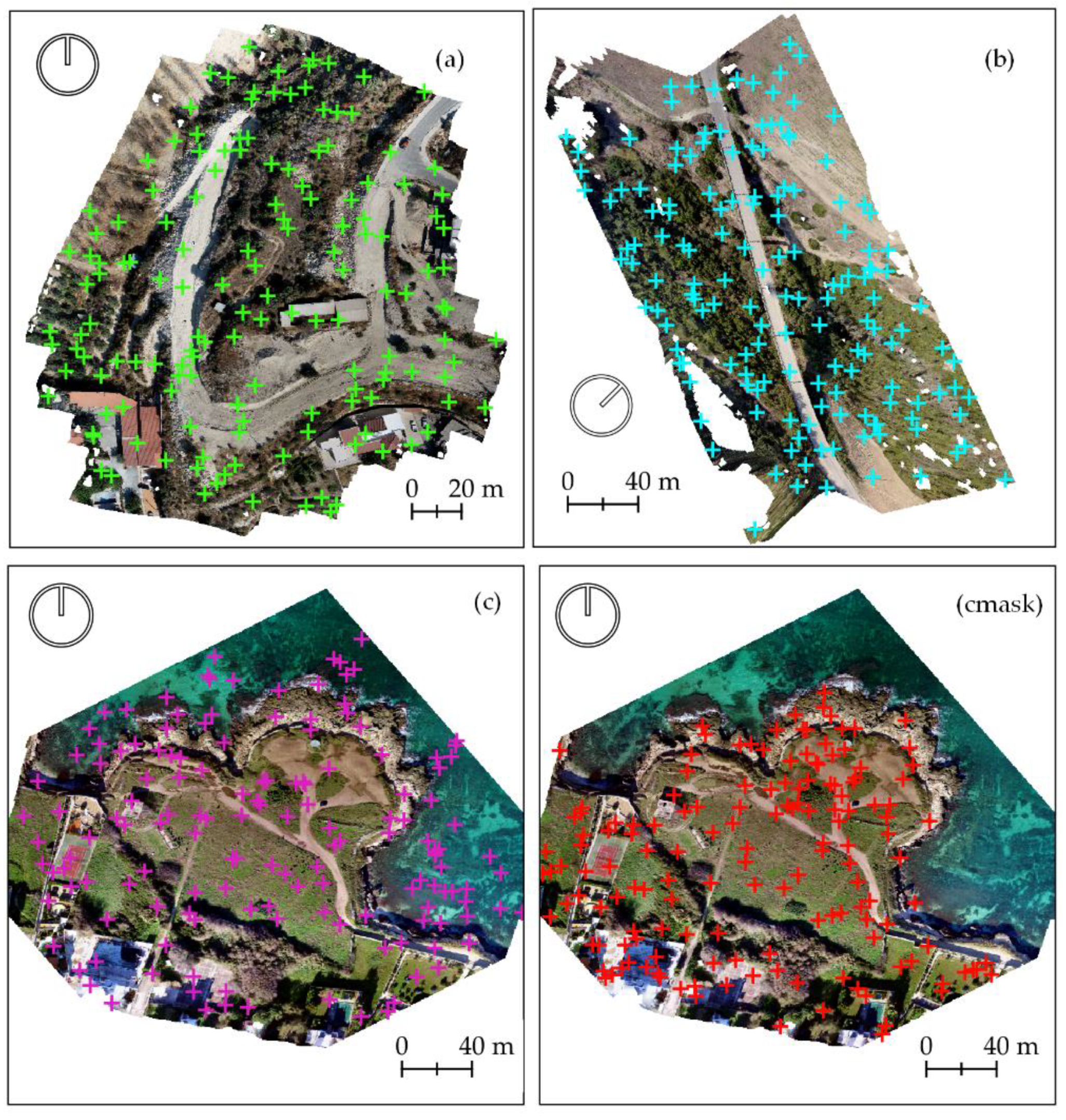
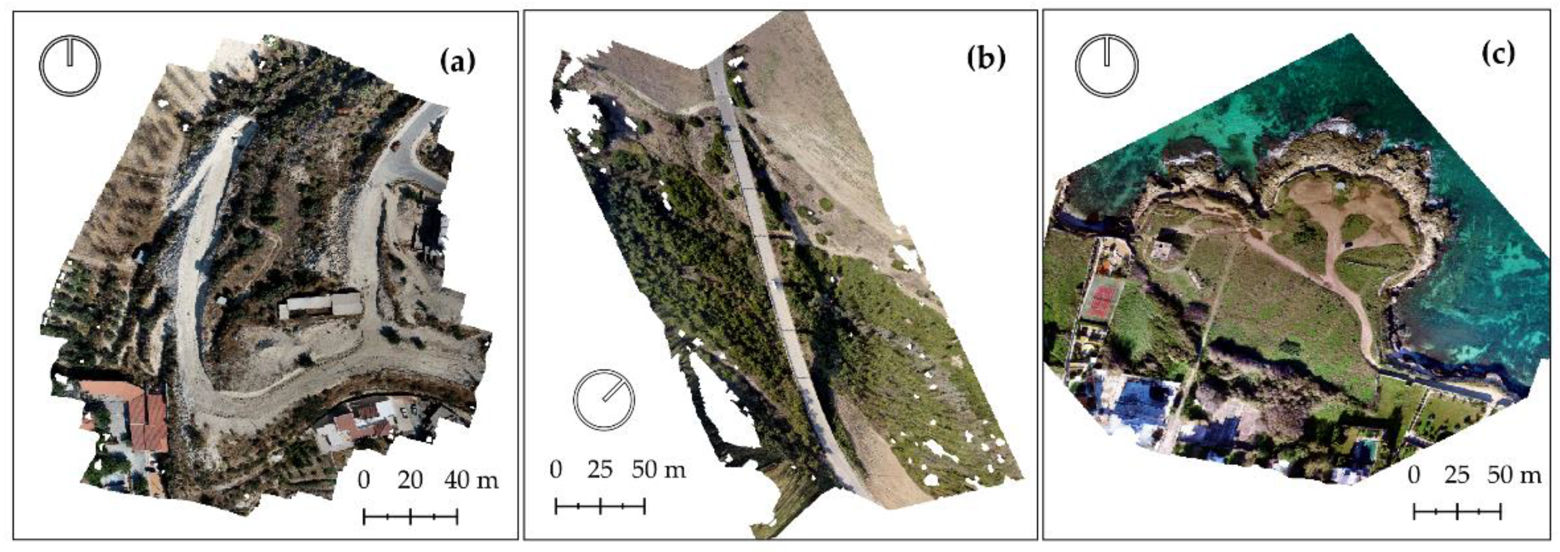
2.1. Acquired Datasets

For the needs of the current study, three different datasets were selected, based on the following criteria: (1) having a different context, (2) being captured by different UAV/camera sensors, (3) having a different georeferencing strategy, and (4) capturing by different altitude above ground level (AGL) and (5) different ground sample distance (GSD). These five connotations among the three datasets allow us to prove the versatility and non-specificity of the workflow proposed in the research. A preview of these areas can be found in Figure 1. Case study (a) was a construction site not far from the village centre of Fasoula in the Limassol district in Cyprus (Figure 1a), where vegetation was randomly scattered. An out-of-town environment in Grottole in the province of Matera (Italy) was selected as case study (b) (Figure 1b), where high vegetation, bare soil, and, above all, a viaduct were visible. An abandoned archaeological area, named Punta Penna because of the promontory on the sea where it stands, in Torre a Mare, the southernmost district of the city of Bari (Italy) was considered as the third case (c) (Figure 1c). It should be mentioned that water was visible in this dataset.
Table 1 shows the characteristics and technologies used for each dataset.
For the second dataset, a GNSS acquisition campaign of 11 ground control points (GCPs) was carried out, measured in network real-time kinematic (nRTK) mode with an average accuracy of 2 cm the three axes, in order to perform an indirect georeferencing of the photogrammetric products. For the rest of the case studies, a direct georeferencing was preferred, i.e., in the first case using the geo-tags of each image measured in RTK using the receiver on board the vehicle (average accuracy of about 10 cm), while in the other case using the same geo-tags but measured with a low-performance GNSS receiver (average accuracy of 3 m).

2.2. Photogrammetric Processing

The processing of the collected datasets was based on the workflow proposed in [14,40,41]. The different parameterisations for each dataset were detailed in this paragraph. Agisoft Metashape software (v.1.4.1, Agisoft LLC -St. Petersburg, Russia) was used during the work on Intel(R) Core (TM) i7-3970X CPU 3.50GHz hardware, with 16GB of RAM and an NVIDIA GeForce GTX 650 graphics card to return the photogrammetric products.
Three chunks were generated, and the workspace was adjusted, as shown in Table 2. The first step was to correctly set up the workspace and remove any blurred images, which could compromise the final results. After launching the estimate image quality tool (Agisoft Metashape), the results obtained with a quality value beyond a threshold equal to 0.7 were included in the processing chain. Briefly, this tool provides information about the sharpest borders detected on the image and can be used to find blurred images. For the third case study, it was necessary to manually fix the GPS/INS Offset value equal to (0.005 ± 0.005, 0.100 ± 0.01, 0.250 ± 0.01) m, concerning the lever-arm vector. In contrast, for the other cases, this was automatically computed and recorded in each geotag by the technology equipped on board each aircraft. No manipulations of the radiometric information were performed, varying illumination and contrast, so as not to compromise the original data.
The sparse point cloud reconstruction was started in the next step, initiating the camera alignment processes as indicated in Table 2. The point clouds obtained were subjected to filtering by indicating thresholds (Table 2), already validated in Saponaro et al. [42], regarding reconstruction uncertainty, projection accuracy, and reprojection error. This allowed the bundle block adjustment (BBA) algorithms, which ran in Optimize Cameras, to transfer initial corrections to the models.
According to the designed strategy (Table 1), a direct or indirect georeferencing of the models was performed, and a final BBA was performed to readjust the model. The primary source of error in georeferencing comes from executing the linear transformation matrix on the model [33]. The mitigation of potential nonlinear deformation components of the model and the minimisation of the sum of the reprojection error and the reference coordinate misalignment were performed by reinitiating the estimated point cloud optimisation camera parameters based on the known reference coordinates.
The point cloud densification algorithms were started as the last step, DEMs were calculated on these and image orthorectifications were generated based on the computed elevations. In general, orthorectification is transforming from a central projection of the original image to a parallel projection [34]. Consequently, displacement due to the tilt of the sensor and to the terrain relief was corrected. The blending mode has two options (mosaic and average) for the mosaicking step to select how pixel values from different (overlapping) images will be combined in the final texture layer. In this study, the selected mosaic options are shown in Table 2. Blending pixel values using mosaic mode does not mix image details of overlapping photos but uses only images where the pixel in question is located within the shortest distance from the image centre [33]. Four orthomosaics were exported for each scenario investigated: beginning from the highest resolution and then doubling, tripling, and quadrupling the resolution. Further down-sampling would not justify the use of UAV technology [43]. In particular, the Agisoft Metashape software made it possible to export the orthomosaics at the chosen resolution, resampling each time by bilinear interpolation.

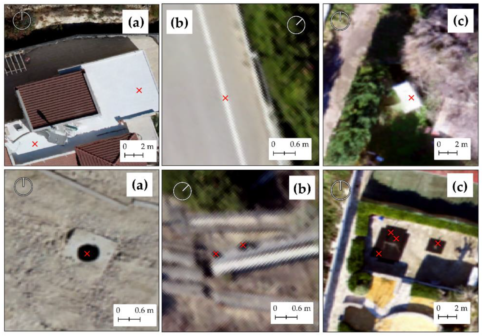
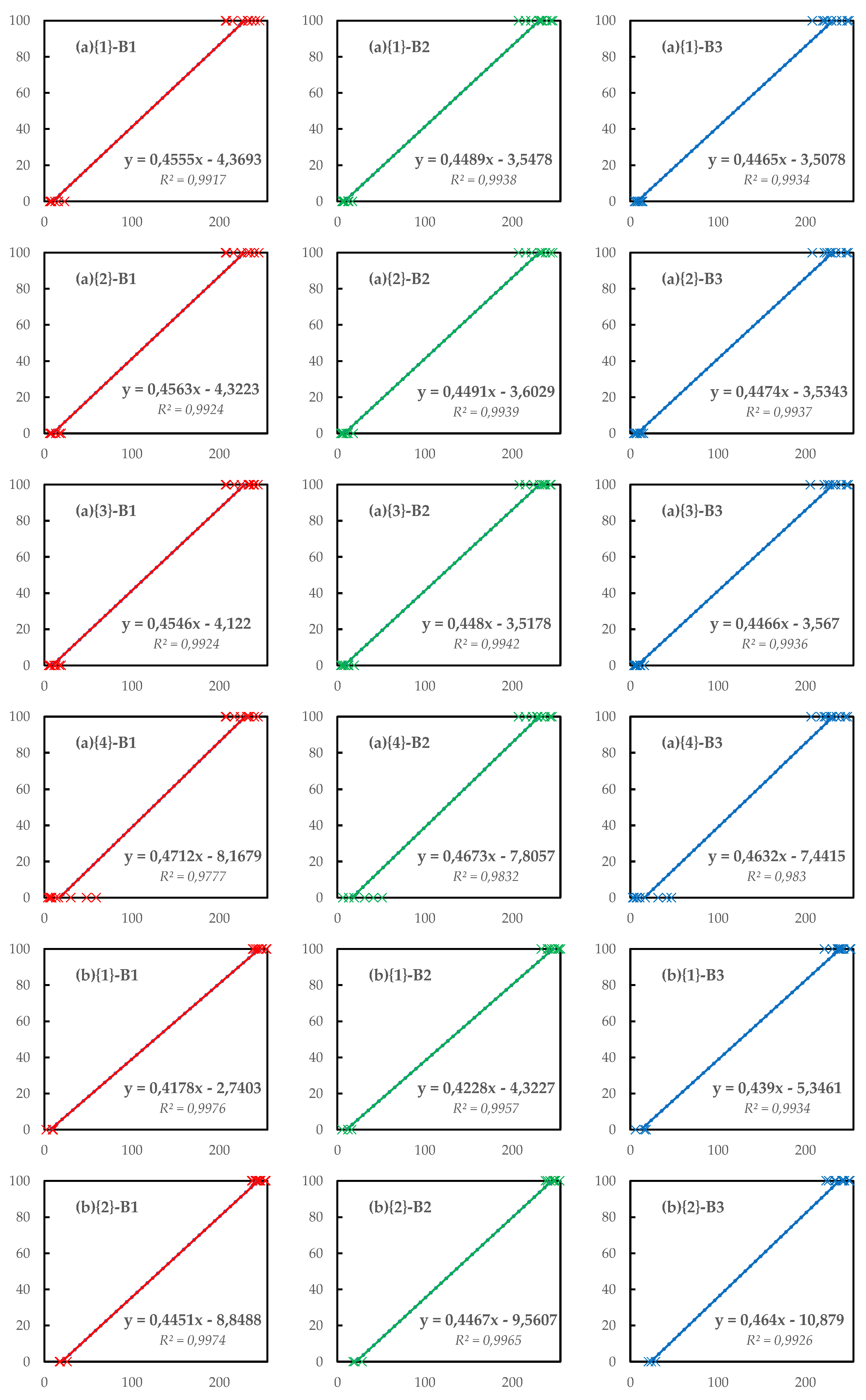
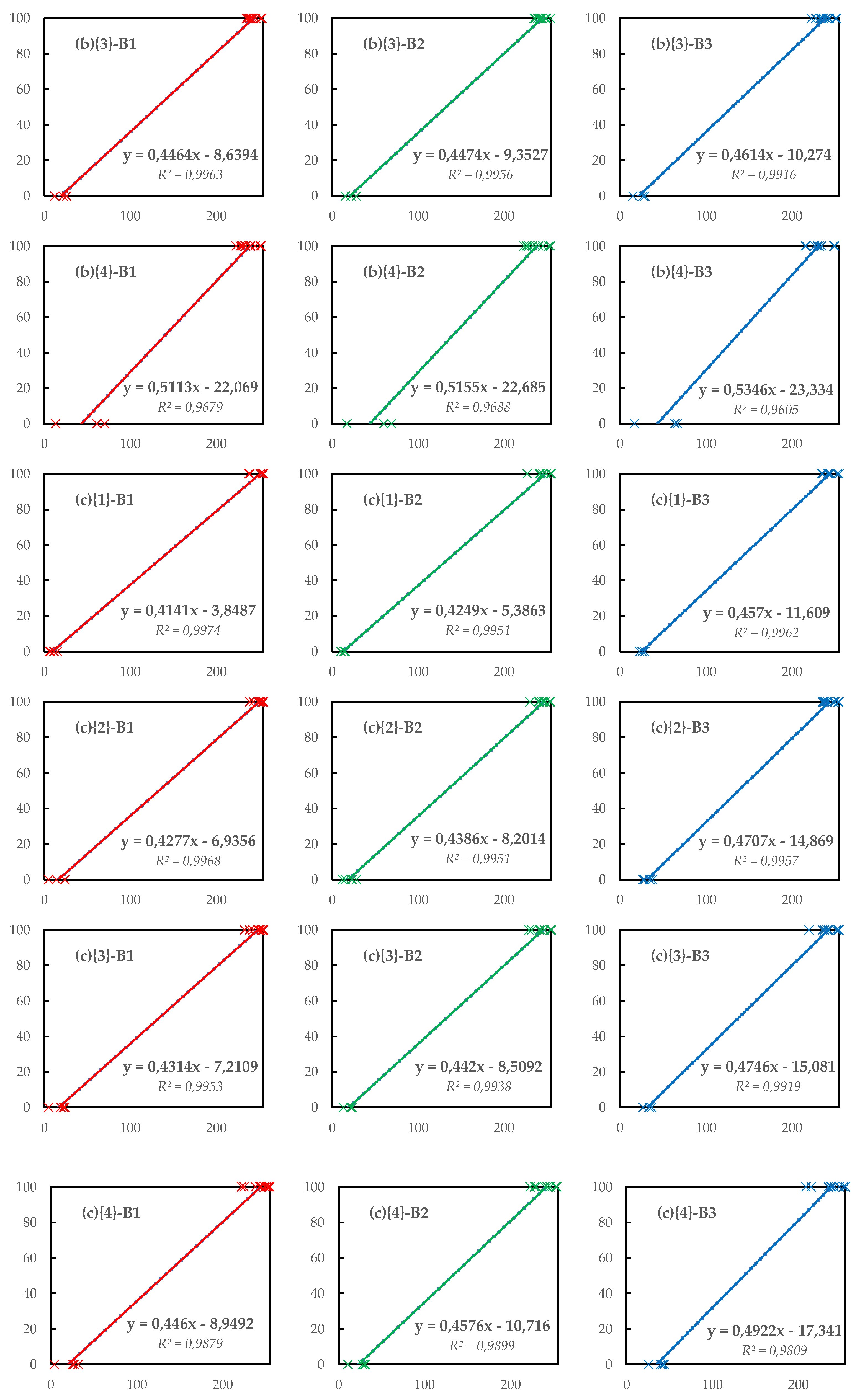
2.3. Empirical Line Method

Prevailing environmental conditions highly influence UAV imagery at the time of data acquisition [10,18]: the atmospheric composition (e.g., water vapour and aerosols) and solar illumination patterns are the most impacting on the radiometric camera calibration.
Consequently, while images of the same scene acquired from the same sensor at different times may have different properties [33], images acquired from the same sensor and campaign may also contain noise due to lens distortions, systematic sensor errors, as well as variation in camera sensitivity across the same image [38].
Therefore, it is essential to carry out a radiometric calibration of the photogrammetrically returned orthomosaics to be considered quantitatively and qualitatively comparable.
The orthomosaics were imported into the open-source software QGIS (3.16.5 ‘Hannover’) [44]. Following the procedures adopted in [29], high and low reflectance targets were manually identified as represented in Figure 2, avoiding points with equivocal exposure.
Consequently, we considered the adequacy of the target sites against the criteria proposed in [34]: (a) high spatial homogeneity, concerning the spatial resolution of the image dataset, i.e. ideally, each target should cover an area of about 5 × 5 pixels in the reference images; (b) representativeness of the dynamic range of the radiance in the region; (c) low adjacency effects of targets located at an adequate distance from other volumetric scattering disturbances; (d) low slope effects, i.e., targets with flat or Lambertian surfaces; (e) low temporal variability of the spectral response, i.e., targets with stable spectral response that do not show rapid changes due to short-term dynamic phenomena.
Using the raw digital number (DN) values per band extrapolated from each target, a linear relationship was constructed by empirically associating to the DNs the extreme percentage values (range 0–100%) of reflectance, low and high, respectively. The method of calibrating the DN of each band is called empirical line method (ELM). Precisely, ELM is a non-rigorous but basic approach to calibrate the DN of images to approximate units of surface reflectance in case no further spectroscopic information is available on the ground [39], as in our work. It then constructs a relationship between sensor radiance and surface reflectance by calculating those nonvarying spectral targets and comparing these measurements to the respective image DNs [4]. Thus, prediction equations were derived that can contemplate changes in illumination and atmospheric effects. Due to the low altitude at which the measurements were taken and the unavailability of precise information, the impact of atmospheric effects was deliberately ignored [29].
The ELM for the RGB UAV sensed data could be estimated using the following linear equation:
ρ ( λ )   =   A     DN   +   B
where ρ (λ) is the reflectance value for a specific band (range 0–100%), DNs are the raw digital numbers of the orthophotos, and A and B are terms which can be determined using a least-square fitting approach [29]. Although it is widely used with reasonable results, radiometric corrections using ELM can introduce noise, and caution should be exercised in its application. Indeed, most digital cameras have built-in algorithms that use a curvilinear function to transform electromagnetic radiation into digital signals in order to simulate the way human eyes perceive grey. Therefore, consumer cameras are designed to take pictures that look good, not to capture scientific data for research. Therefore, the relationship between surface reflectance and raw image DNs remains poorly decipherable for these cameras [4]. Goodness-of-fit measures, such as the coefficient of determination (R2), were used to assess the accuracy of the ELM correction so that the regression’s suitability could be quantitatively proven [34].
The A and B values of Equation (1) were estimated and used in the raster calculator in QGIS software to perform each band’s radiometric calibration. To validate the consistency of the performed calibrations, 15 points per scenario were manually identified among vegetation, bare soil, and asphalt. Their spectral signatures were compared with those commonly accepted in the literature.

2.4. Vegetation Indices

Once the orthomosaics were radiometrically calibrated, various visible vegetation indices were computed with pixel values ranging between 0 and 1. The ten (10) VIs used in this work and their formulas are shown below. In particular, referring to the study carried out in [29], the following vegetation indices were assessed to all case studies:
  • Normalized green–red difference index (NGRDI) [45]
( ρ G ρ R ) / ( ρ G + ρ R ) ,
  • Green leaf index (GLI) [46]
( 2 ρ G ρ R ρ B ) / ( 2 ρ G + ρ R + ρ B )
  • Visible atmospherically resistant index (VARI) [47]
( ρ G ρ R ) / ( ρ G + ρ R ρ B )
  • Triangular greenness index (TGI) [48]
0.5 [ ( λ R λ B ) ( ρ R ρ G ) ( λ R λ G ) ( ρ R ρ B ) ]
  • Red–green ratio index (IRG) [49]
ρ R ρ G
  • Red–green–blue vegetation index (RGBVI) [50]
( ρ G   ρ G ) ( ρ R ρ B ) / ( ρ G   ρ G ) + ( ρ R ρ B )
  • Red–green ratio index (RGRI) [51]
ρ R / ρ G
  • Modified green–red vegetation index (MGRVI) [50]
( ρ G 2 ρ R 2 ) / ( ρ G 2 + ρ R 2 )
  • Excess green index (ExG) [52]
2 ρ G ρ R ρ B
  • Colour index of vegetation (CIVE) [53]
0.441 ρ R 0.881 ρ G + 0.385 ρ B + 18.787
where ρ B is the reflectance at the blue band, ρ G is the reflectance at the green band, ρ R is the reflectance at the red band, λ B is the wavelength of the blue band, λ G is the wavelength of the green band, and λ R is the wavelength of the red band.
As can be seen in Equation (5) to calculate the TGI index, the peak wavelength sensitivity of the RGB camera was required. Therefore, the index calculation still depends on the assumption that the user knows the peak wavelength sensitivity of the camera used. Low-cost RGB cameras were not supplied with the specifications of the mounted CMOS sensors, as in our cases [17]. It was therefore chosen to set default values for all cases to λ B = 480 nm, λ G = 560 nm, and λ R = 655 nm.
The results were then analysed and compared using 150 random points automatically identified in the orthomosaics [54,55].

2.5. Classification Algorithm Feedback

The raster files concerning the radiometrically corrected RGB bands and the maps concerning the VIs, which were the most significant in terms of results as subsequently explained in Section 3.3, were imported into the Sentinel Application Platform (SNAP) software [56]. Actually, this is a common open-source architecture for ESA Toolboxes ideal for the exploitation of earth observation data. As its name implies, it is mainly designed for processing data concerning Copernicus Sentinel missions [56], but it is functional for different operations on different data as well [54,55].
SNAP integrates a multitude of tools for exploring and processing multisource data. For the purposes of this work, this platform offers the possibility to run supervised classification algorithms. Among these, random forest (RF) is a widespread supervised classification and tree regression technique [57]. Specifically, the RF algorithm randomly and iteratively samples data and variables to generate a large set, called a forest, of classification and regression trees [58]. The classification output describes the statistics of many decision trees, resulting in a more robust model than can be obtained from a single decision tree produced by a single execution of the technique [57]. Thus, the regression output from RF effectively represents the average of all regression trees grown in parallel without pruning [59]. The iterative nature of RF gives it a distinct advantage over other methods in that the data is effectively bootstrapped, thus feeding random subsets of the training data, to obtain more robust predictions and reducing the correlation between trees [60].
For each scenario, containers of vectors were generated for the training areas about the classes’ vegetation, asphalt, and bare soil. For each class, 10 areas were manually drawn uniformly distributed over the whole scenario and including the radiometric heterogeneity of each class. Subsequently, 30 pins were placed for each class, which will act as validation points, i.e., pixels whose membership of a class is certified and whose classification prediction is verified. The RF algorithms were carried out using the generated training areas and using only the RGB bands as resources first, after which the information from the most significant vegetation maps, calculated in the previous step, was added. From the results extracted for each scenario, at the different resolutions, according to the criteria defined in [61], the confusion matrices and F-scores [62] for each class were arranged.
The F score proves to be an efficient metric of the accuracy of a test [62]. It is calculated from the combination of precision and recall of the test: precision is the number of true positive results divided by the number of all positive results, including those not correctly identified, while recall is the number of true positive results divided by the number of all samples that should have been identified as positive. The score takes values in the range from 0 to 1, where the latter represents perfect accuracy and recall, while in the opposite case accuracy is poor and reorganisation of the classification process is inevitable.

3. Results

Based on the photogrammetric processing chain described in Section 2.2, four orthomosaic solutions were exported for each scenario investigated. The spatial resolutions (m/pixel) established were reported in Table 3. Imported into the open-source platform QGIS, each orthomosaic underwent the same processing workflow.

3.1. Radiometric Calibration of the Raw Orthophotos

Figure 3 shows the empirical lines obtained and the respective equations after the implementation of the ELM method. The coefficient of determination R2 for each regressed empirical line showed an optimal prediction condition among the manually chosen points. Comparing the R2 values obtained at varying spatial resolutions, the values are somewhat comparable. There is a slight, but not significant, decrease only in the solution {4}, thus indicating an increase in prediction errors. Future investigations could examine stronger down-sampling cases, thus identifying possible limitations of the methodology in finding these regression lines.
The values of coefficients A and B, as given in equation (1), derived from the regression line equations in Figure 3, were used for the radiometric calibration of each band of each resolution solution listed in Table 3.
To confirm the radiometric correction, the reflectance values of each calibrated raster were extracted, and the spectral signatures of points falling in vegetated areas, in asphalt, and bare soil were constructed (Figure 4).
As already described by [29], an unambiguous trend among the various selected points was difficult to extrapolate. Even in this process chain, it was not deemed necessary to distinguish among different behaviours by class. For example, in the case of vegetation points, no distinction was made between type and state of health, while for asphalts, the age of laying was not known. It was possible to state that the trends described in Figure 4 reasonably track behaviour observed in the literature [29,34].

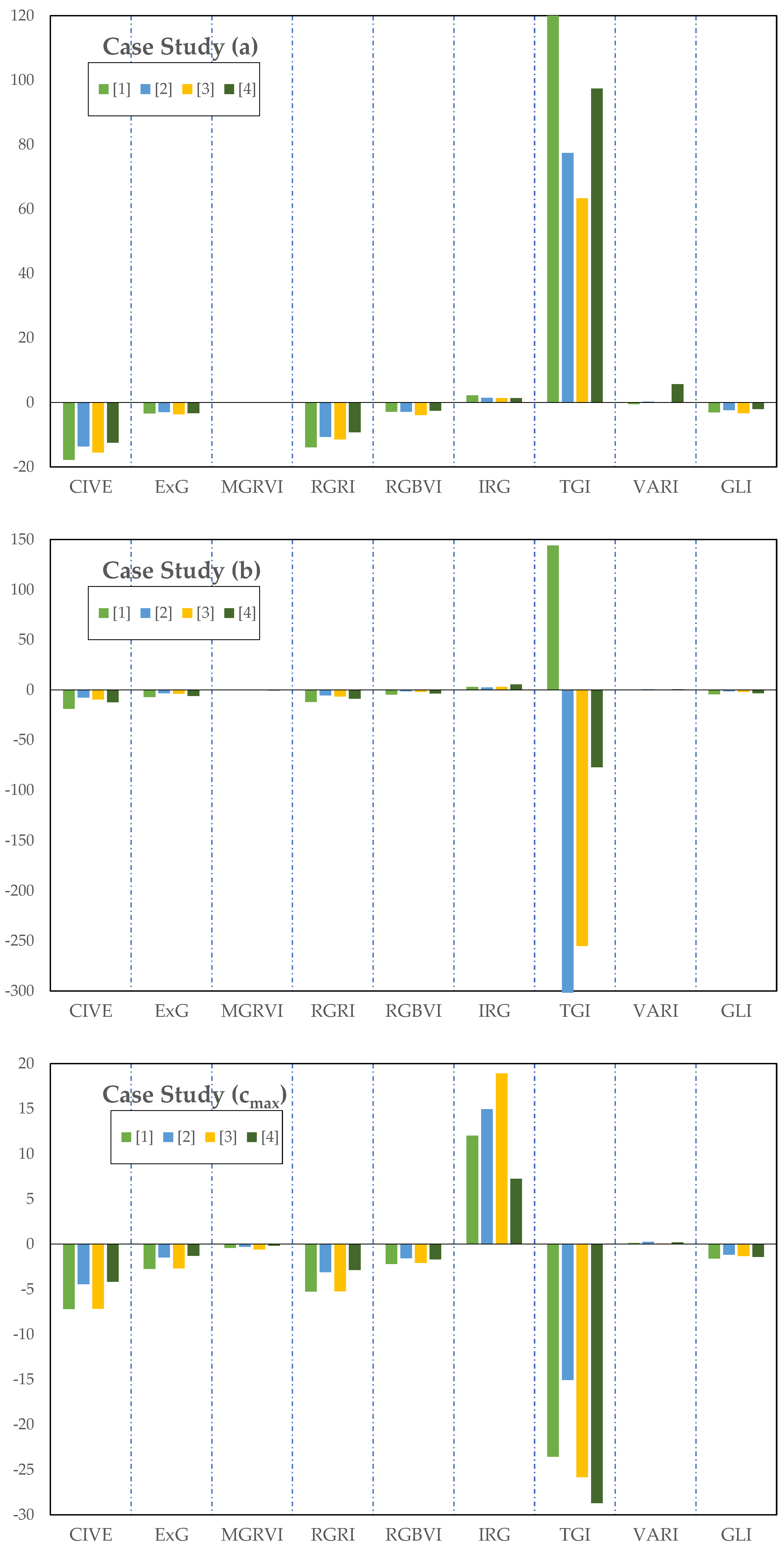
3.2. Vegetation Indices
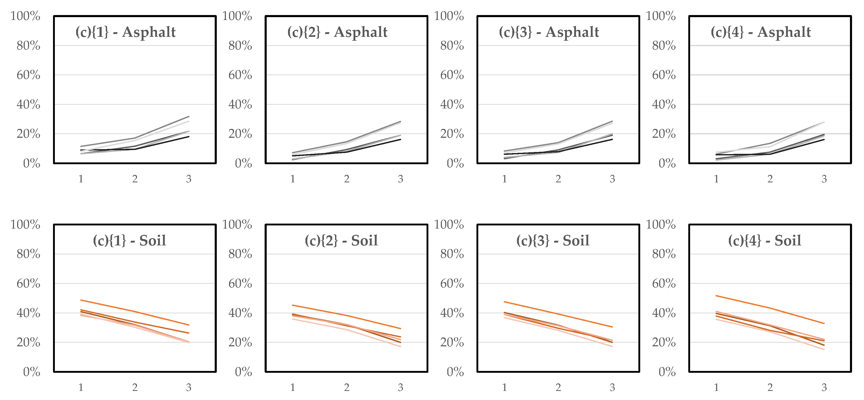
After obtaining the radiometrically calibrated raster files of each band for each solution, the ten (10) vegetation indices listed in Section 2.3 were calculated. To validate the results, 150 random points were located, as shown in Figure 5. Figure 6 shows a distribution of these points between points in vegetated and non-vegetated areas. When classifying these points, points with reflectance values per band outside the range (0:1) were removed. These points suffer from the methodology of radiometric calibration of the images, which, as set out in Section 2.4, is still a raw and not entirely effective method. At other points, distortions caused by the low quality of the sensors and/or artefacts generated by the SfM-MVS procedures result in fallacious reflectance values [13]. The vegetation indices for all points were thus estimated.

3.3. Statistics

Given the distinction between points in vegetated and non-vegetated areas (Figure 6), the two statistical populations for each VI, for each resolution solution and scenario, were subjected to a t-test with a 95% confidence level to interrogate their significance for subsequent statistical inferences. Therefore, the latter presented acceptable and not acceptable results in terms of significance relative to the chosen confidence level. In particular, the not acceptable results already attested to a complete inability to separate vegetated and non-vegetated areas since the mean values of the indices cannot be defined independent.
The normalised difference between the mean value V I ¯ for each index over vegetated areas and nonvegetated areas:
V I ¯ V e g e t a t e d V I ¯ N o n   V e g e t a t e d max ( V I V e g e t a t e d )
represents the adopted descriptor of the propensity of each vegetation index to attesting separability in the extraction of the above classes. The results were presented in Table 4. Blue indicates negative normalised difference value, while red indicates positive value per vegetation index for each spatial resolution. Lighter colours thus indicate a low degree of separability. The acronym NA identifies not acceptable results, defined above, due to differences between the means of the indices that are not significant for the 95% confidence level adopted in the t-test.
Overall, the limit values of the normalized difference range from a minimum of −675.3% to 304.9% for all indices in solution {1}, from −482.1% to 3123.2% in {2}, from −350% to 6337.3% in {3} and finally from −654.8% to 595.3% in solution {4}. The extreme values of these ranges were found in the TGI index in all analysed resolutions. In general, the remainder were more moderate values. The overall analysis of the ratio between not acceptable and acceptable values returned by the t-test was 0.45 in case {1}, 0.40 in {2}, 0.325 in {3} and 0.35 in {4}. The optimal resolution for obtaining a greater number of vegetation indices at a 95% confidence level of the t-test was identified in {3}.
The results obtained in the (a) case of Fasoula (Cyprus) showed a higher mean acceptability ratio in the t-test equal to 0.175. Regular surfaces, low vegetation, and clearly distinguishable feature point certainly make orthomosaics more workable for vegetation indices. Subsequently, a somewhat comparable average acceptability ratio was found in the scenario (cmask). In this case, a ratio of 0.2 was recorded between acceptable and not acceptable values in all resolutions. In particular, the masking of the water areas from the orthomosaic improves their interpretability by the indices, returning acceptable values of separability between the classes investigated. Case (c) showed a mean ratio of 0.65 between the analysed resolutions. Particularly remarkable were the values assumed by the IRG index (cmask), compared with the corresponding NA results in case (c). For the following statistics, it was therefore preferable to focus on the (cmask) case.
Last, case (b) was characterised by an average acceptability ratio of 0.5. Only the latter scenario showed a linear improvement in the acceptability ratio as the spatial resolution decreases.
The highest magnitude was recorded in case (c){3}, so without masking, about the TGI index with a value of 6337.3%. Besides, this index presented the acceptability ratio equal to 0, showing itself to be functional in all cases and taking on very consistent values.
The ExG index looked functional in each scenario (ratio equal to 0) and at each resolution adopted: the most significant scores were presented in scenarios (b) and (cmask). Noted a percentage deviation of more than 20% between scenarios (c) and (cmask).
The VARI index was not acceptable for all cases analysed, except for case (b) at resolution {4}, thus presenting the highest ratio of 0.9375 among the indices. Moreover, it did not have a score such that it can be considered functional in the separability between classes. As already resulted in [29], the CIVE (ratio 0.0625) index obtained the lowest score for all the resolution solutions in each scenario; among them, the scenario (cmask) is the most reactive. The NGRDI behaved similarly to the VARI index and was only acceptable in resolutions {2} and {3} of scenarios (a) and (c), with insignificant scores below 15%. Its acceptability ratio was 0.75.
Scenario (c) did not respond to the MGRVI (ratio 0.4375), RGRI (r. 0.4375), RGBVI (r. 0.375), IRG (r. 0.3125), and GLI (r. 0.4375) indices, while significant scores were obtained in both (cmask) and (a), except for the RGRI index in the latter scenario. Noteworthy values were recorded in scenario (cmask) for the IRG index.
In general, the case study (cmax) (archaeological area with water masking) tended to give high differences between vegetated and non-vegetated areas regardless of the applied vegetation index, indicating that postprocessing of the images by removing areas of ambiguity, such as water, optimises interpretability in the analysis. It was not possible to identify the most challenging environment to work with and try to discriminate vegetation from other areas at any resolution solution. The general trend suggested that as the sampling frequency increases, lower resolutions reduce ambiguities or noise in vegetated areas, thus improving discriminability. From Table 4, it can be deduced that within the same trend, some resolutions work better than other lower resolutions and are therefore optimal in describing the radiometric information.
Based on the results of Table 4, a performance comparison between indices was set up, i.e., a normalised difference for all case studies between all vegetation indices referenced to the NGRDI index. The results of this analysis were shown in Figure 7 for each scenario in the various spatial resolution solutions. The normalised difference indicated the percentage difference between:
V I ¯ V e g e t a t e d i N G R D I ¯ V e g e t a t e d N G R D I ¯ V e g e t a t e d
where each mean value was normalised to the maximum value of each index among vegetated points, therefore, in Figure 7, high values imply that the VIi index performed better than the NGRDI index; on the contrary, negative values suggest that the specific index performed worse. Trivially, vegetation indices around zero have comparable performance with the reference index.
From the results in Figure 7, it was observed that the IRG index performed positively in comparison to the NGRDI index for all case studies in any resolution solution. In most cases, the VARI index also exhibited positive behaviour relative to the reference index, except for scenario (a) in resolution {1} in which it takes on a negative but near-zero value of −0.48%. However, the IRG and VARI performance did not show efficiencies of more than 10%, and in the case of the VARI index, this is almost as good as the NGRDI index. On the other hand, given the considerations from Table 4, the VARI index cannot be considered completely efficient. With its acceptability ratio of 0.3125, the IRG index was shown to be non-functional in scenario (c). Therefore, it is based on Figure 7, efficient for this work. The latter presents a slightly decreasing efficiency in the case study (a), increasing in case (b) and peaking at resolution {3} in case (cmax).
An irregular performance was that of the TGI vegetation index as it provided for case (a) returns of over 60%, up to a maximum of 121% in the different resolutions, while for cases (b) and (cmax) very negative values, except case study (b) at the first resolution {1} where it even reached a value of 144%.
The remainder of the calculated vegetation indices, on the other hand, show negative returns compared to the reference index: not excessively high values of less than −20%. It was not possible to describe a normal behaviour of the efficiency of the indices as the adopted resolution varies. In this regard, Agapiou [29] stated that for each case study, the optimal index is not unique, which is also in line with the previous results in Table 4. Thus, it is not possible to deduce a direct relationship between the resolution of the orthomosaic and the index returned.

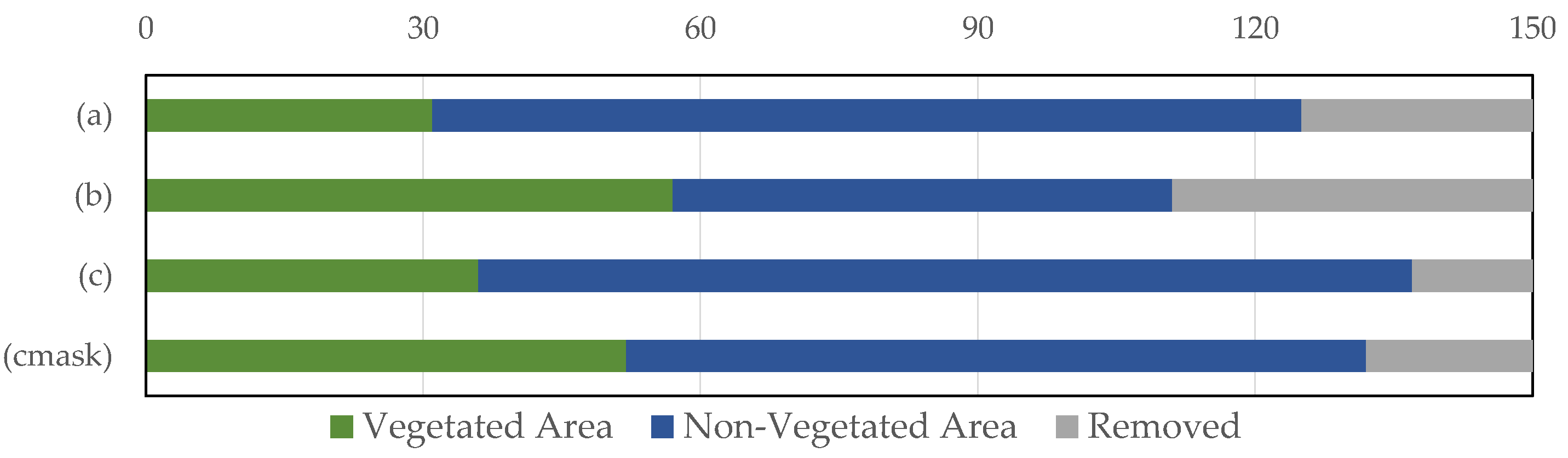
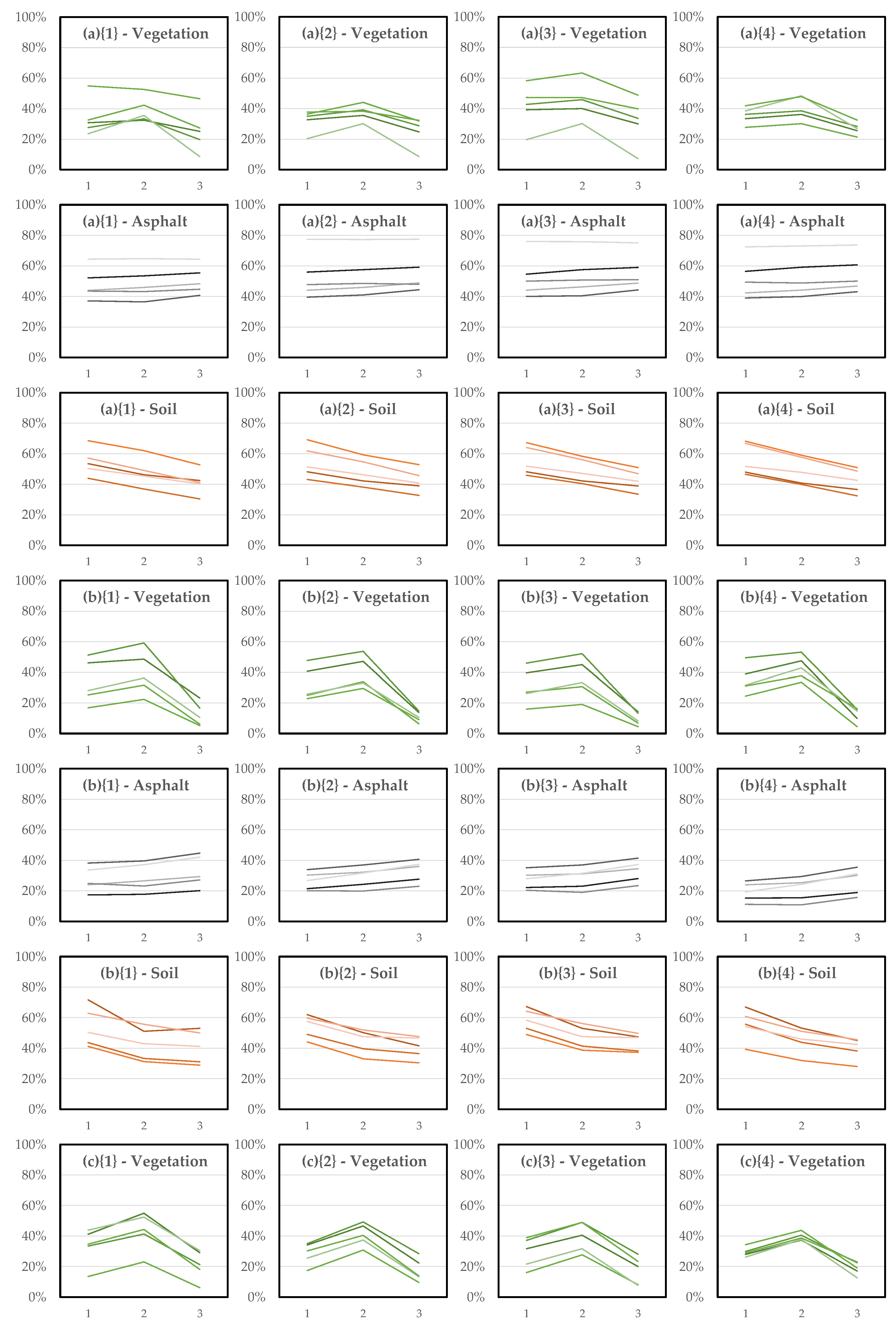
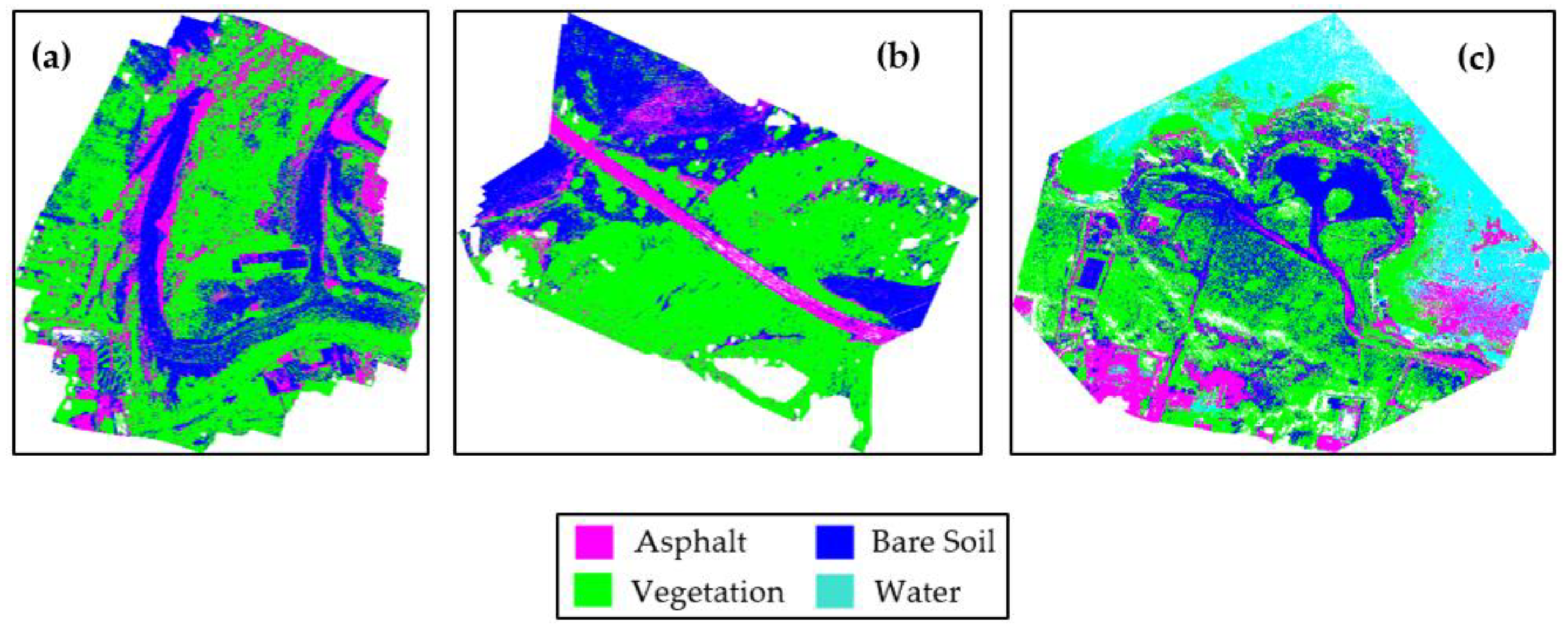
3.4. Supervised Classification Responses

After performing the supervised classification procedures using the RF algorithms, the validation metrics were extracted. In particular, considering the comparison between the labelling assigned and that predicted by the software in the 90 pins placed, for each scenario, at each resolution and for each classification mode (RGB bands, adding the TGI band, adding the IRG band), the confusion matrices were extracted and from these the F-Scores were computed. In Table 5, the F-Scores were summarised for each class: vegetation (V), asphalt (A) and bare soil (B). In the present examination of the third scenario, the unmasked data (c) was preferred in order to analyse the performance of the classification algorithms at a basic level of image processing, i.e., only radiometrically corrected.
In view of the results shown in Table 4 and Figure 7 in Section 3.3, a reasonable interest in the vegetative indices TGI and IRG and their behaviour was inferred. While the TGI index was taken on significant values in Figure 7, these were not positive in all cases. On the other hand, the IRG index, although with much smaller values, always presents effective values. The classifications were therefore carried out by first using only the radiometrically corrected RGB bands, then the TGI and IRG vegetation maps were used as additional resources separately. In Table 4, the TGI index showed the maximum acceptability ratio, i.e., it was continually functional with always significant values. While the IRG index did not work for scenario (c), it reactivated for scenario (cmask) such that the interest in the results obtainable from the classification in (c) increases.
Given the considerations stated in Section 3.1, a coarse radiometric calibration such as that by ELM does not allow a clear distinction to be made between and in the image components. This translates in the classification into a reduction of the ability to distinguish classes such as asphalt and bare ground, which in several cases may have spectral similarities (e.g., as in the case of very old asphalt). As can be observed in Table 5, the low F-score values (minimum case of 0.33 for A in (c), {1}, +IRG band) are attributable to these two classes, while the class concerning vegetation presents values always higher than the minimum 0.67, found in case (a), spatial resolution {4}, +IRG band mode. The highest F-score value of 0.98 was computed for four cases of vegetation at resolutions {2}, {3}, {4} in the classifications with vegetation indices and all in scenario (b). While the algorithms are facilitated in this scenario by the high presence of vegetation, the resolution {1} is found to be less effective due to the presence of noise and distortions in the pixels.
Focusing on scenario (a), it is evident that the launched classifications, at all the analysed resolutions, benefited from the TGI index while the IRG index produced limited negative effects with respect to the RGB base case. Contrary to the predictions dictated by Table 4 and Figure 7 that noticed the case {4}, the spatial resolution case {2} using the TGI index was the most efficient in terms of performance. Indeed, the lower resolution case {4} was almost comparable in terms of average performance but the RF algorithms implemented in the SNAP software benefited from the better resolution of {2} to build better decision trees.
In scenario (b), the values obtained in all cases were noteworthy, but those obtained using the vegetative indices stand out. It was not possible to identify a unique trend among these and at each resolution the F-scores vary producing for each class limited positive or negative effects. In general, the lower resolution produced more significant values, supporting the hypothesis that a reduction in resolution reduces the distortions and noise in pixels caused by SfM techniques. Among all cases, the RF algorithms produced the most effective results using the IRG information in solution {4}. In comparison with the results obtained in the previous section, this product can be considered consistent with the performance of the discussed statistics.
Finally, scenario (c) presented some emblematic values. In particular, although the F-score values for the vegetation class were considered valid in all cases, the other two classes presented very fluctuating values, reaching values even lower than 0.5. From the point of view of the vegetation class extraction, the highest F-score value was shown by using the TGI index in the {3} solution, as also demonstrated in Table 4. In fact, this latter resolution presented the highest performance values, proving to be optimal for the classifications of this scenario. Among these, the most efficient case for the three classes analysed was the one that used only the RGB bands during classification. This demonstrates, once again, that in this scenario the usable indices can only become more significant after a masking procedure.
Figure 8 shows the most successful classification maps obtained.

4. Discussion

The results shown in the previous section provide some useful considerations to prepare an interesting discussion about vegetation extraction in orthomosaics, in various environments and at various spatial resolution solutions.
The application of vegetation indices based on visible bands, perhaps of a nonmetric camera, highlights the potential for discriminating vegetated areas widespread and routine. Hence, to understand their limitations and efficiencies, the results presented in Table 4 indicated the behaviour of different indices in performing high or low separability between vegetated and non-vegetated areas. In several cases, even some indices could not return significant values and therefore not acceptable at the 95% confidence level of the t-test. As already documented in other recent works [18,25,29], it has been shown that there cannot be a single index performing in the same way for the various case studies. Consequently, it was apparent that each index is suitable for particular environmental contexts. Thus, there is a need to generate an abundant collection of cases to statistically deduce any similarities between the various indices and the analysed contexts.
In this regard, the values of the average acceptability ratios allowed us to deduce certain issues. The context of some orthomosaics can be quite complex, such as the case study (c). The results learned in Table 4 showed how the masking of highly ambiguous areas, such as areas with the presence of water, completely improves the interpretability of the images. This was also demonstrated by the results obtained in Table 5 about the efficiency of the classifications. Indeed, masking leads to the exclusion of false-positive points. Differences in the sensitivity of cameras to capture backscattered reflection values in specific wavelengths can be significant, as has been shown in the past by other studies [38]. In addition to the spectral complexity and heterogeneity of the scenario, some other factors can affect the indices’ overall performance: e.g., inhomogeneous lighting (low-clouds effect), sun exposure (shaded and partially sunny areas), and presence of dense vegetation. In scenario (b), photogrammetric processing of densely vegetated areas generated many noisy and distorted areas. Generally, these areas appeared as a constant source of reconstruction errors due to the low efficiency of SfM techniques in defining unambiguous points. The matching algorithms are weak in identifying stable tie points in vegetated areas, which generates artefacts and distortions that are challenging to resolve [13]. As shown in Table 4, this set off a loss of efficiency of extraction techniques in vegetated areas. In Table 5, however, it is shown how a lower spatial resolution can benefit the classification results, as distortions and noise are reduced in the subsampling. Scenario (a) proved to be more advantageous in applying the vegetation indices as it was characterised, albeit with a heterogeneous context, by different points and areas not subjected to high noise. On the other hand, only in this scenario is the TGI index considered very incisive, given the observations deduced from Table 4 and Table 5 and Figure 7. This supports what had already been stated: the efficiency of one vegetation index less being than another is indeed linked to the context detected. Another important finding in this matter was that in cases where a ratio between combinations of visible bands was included in the formulation of indices (Equations (2)–(4), (7)–(9)), these did not produce acceptable results in scenarios (b) and (c).
Recent studies [20] have shown that the optimal resolution for remote sensing applications was related to the spatial characteristics of the targets under examination and their spectral properties. Indeed, in [20] the high resolution of an orthomosaic was not always optimal for a given vegetation index in the various case studies. Using low-cost camera sensors, it is assumed that there are overlaps among channels that cannot independently record distinct ranges of wavelengths. As no information on this is available, however, it is not possible to measure its relevance. This issue first was transmitted to the radiometric information recorded in the pixels and subsequently to the formulation of the indices, whose components thus become correlated, as indeed observed.
Considering Table 4, the resolution {3} presented a reasonable acceptability ratio for all scenarios and this was also revealed in Table 5 about the results of the classification. This was not consistent with the magnitude of separability of the examined indices and the efficiency concerning the NGRDI reference index (Figure 7). Actually, a reduction in the spatial resolution smoothens out any noises or distortions caused in the photogrammetric generation of orthomosaics or derived from the poor quality of the starting images. In contrast, looking at Figure 7, it was therefore evident that each vegetation index does not have a unique behaviour when the resolution changes: each of them has an optimal resolution for each analysed context, thus indicating the complexity of extrapolating a direct relationship between these parameters.
Comparing the observations of Table 4 and Figure 7, only the IRG index presents profitable characteristics for all scenarios in each resolution solution. Although its efficiency compared to the NGRDI was less than −5%, wide use of the ExG index cannot be excluded. This was indeed consistent in discriminating vegetated areas in any context and any resolution solution.
A key step was to obtain an overview of the impacts of processing and statistics on pixel-based classification algorithms. Analysing the metrics computed from the confusion matrices (Table 5), no linear dependence between the spatial resolutions and the incidence of the bands used in the classification was noticeable. Indeed, this incidence itself depends on the analysed scenario and as highlighted in (c), some manipulations of the dataset at the base level can improve its interpretability by the classification algorithms. In all the analysed cases, the orthomosaics obtained from photogrammetric surveys can be considered valid tools for the vegetation extraction, while the distinction between non-vegetation classes was more difficult. Finally, this processing chain was a valid expedient for the extraction of vegetation classes, accessible to a wide range of users and application cases.

5. Conclusions

A large body of literature notes the potential and versatility of UAVs. The use of these relatively low-cost platforms combined with the strong development of SfM-MVS techniques can return a wide range of photogrammetric products, including high-resolution orthomosaics i.e., higher resolution than traditional aerial or satellite observations, of small and medium areas. In many applications mainly related to the monitoring of agricultural areas, forests, etc., the ability to discriminate and extract vegetated areas is indispensable. The use of sophisticated sensors capable of capturing spectral information in the near-infrared band would facilitate operations. However, in most cases, UAVs are equipped with low-cost sensors sensitive to the visible part of the spectrum (RGB), making the detection of vegetated areas quite challenging. Furthermore, when working with radiometric information, the images’ radiometric calibration is indispensable to convert the raw digital numbers (DN) into reflectance values. In robust terms, calibration requires field campaigns of a spectroscopic survey of defined targets to obtain a good approximation of the backscattered radiance of the same targets later observed in the images.
In this work, the ELM radiometric correction technique of orthomosaics generated from images acquired by UAV of three different case studies, with different contexts, RGB sensors, and different spatial resolution solutions has been explored. This easily applicable procedure does not require any knowledge of ground targets or field campaigns with spectroradiometers and spectral reflectance targets. The calibrations applied to the various cases screened returned spectral signatures of control points extracted in vegetation areas, asphalt, and bare soil in line with those widely accepted in other literature.
Ten VIs, sensitive in the visible part of the spectrum, were computed based on the visible bands. The results were further manipulated to examine the performance of each index and then to quantify their impacts on the RF supervised classification procedures. From the results of this study, the following aspects can be highlighted:
  • The performance of each index varied for each case study, as already observed in other works. Therefore, to estimate the performance of the indices in general, it is essential to construct a broad case history covering as many contexts as possible.
  • The TGI index, able to return very significant and functional values in terms of separability between vegetated and non-vegetated areas, performs better than the NGRDI index, taken as a reference, only in a regular context without ambiguous areas. The IRG index, on the other hand, performs well in all scenarios but with moderate performance.
  • High resolution of an orthomosaic was not frequently optimal for vegetation indices in the various case studies; by reducing the resolution, the noise in each pixel is smoothened out, improving the radiometric information. In fact, the classification algorithms gave optimal results for {3} resolutions, demonstrating that very high-resolution datasets are not always a guarantee of more precise results.
  • The masking of areas that are strongly characterised by ambiguity, such as those in the presence of water, improves their interpretability by the indices and increases their performance.
  • In areas with dense vegetation, the reduced ability of SfM-MVS techniques to establish and triangulate unambiguous junction points produces artefacts or obvious distortions that compromise VIs’ performance in extracting correct information.
  • Looking at the average performance of the RF classification algorithms, for each case analysed, it emerged that RGB orthomosaics can be considered a valid source for generic vegetation extraction.
This study’s results can be applied to any RGB orthomosaic, taken from a low-altitude system or aerial imagery. The large fleet of low-cost ready-to-fly (RTF) UAVs equipped mainly with inexpensive RGB sensors will continue to grow, and using the approach adopted in this work is an opportunity to exploit the masses of data that can be acquired fully. In the future, targeted VIs will be developed to address specific needs, making vegetation extraction a simpler and more straightforward procedure.
Given the considerations learned about the behaviour of the VIs at varying spatial resolution, more insights can be addressed in future studies about the variability of the same vegetation indices based on visible bands about multitemporal UAV acquisitions of the same scenario.

Author Contributions

Conceptualisation: D.G.H. and E.T.; methodology, A.A. and E.T.; software, A.A. and M.S.; validation, D.G.H. and A.A.; formal analysis, A.A. and E.T.; investigation, A.A. and M.S.; resources, M.S. and A.A.; data curation, M.S.; writing—original draft preparation, M.S.; supervision, D.G.H. and E.T. All authors have read and agreed to the published version of the manuscript.

Funding

This research was funded by Ministero dell’Istruzione, dell’Università e della Ricerca (MIUR)—PON Ricerca e Innovazione 2014–2020, grant number DOT130UZWT.

Institutional Review Board Statement

Not applicable.

Informed Consent Statement

Not applicable.

Data Availability Statement

Not Applicable.

Acknowledgments

We need to acknowledge Michalis Christoforou from the Cyprus University of Technology for the UAV provided at the case study in Fasoula, Cyprus. The authors would like to acknowledge also the ‘EXCELSIOR’: ERATOSTHENES: EΧcellence Research Centre for Earth Surveillance and Space-Based Monitoring of the Environment H2020 Widespread Teaming project for the support of the PhD activities of MS at the Cyprus University of Technology. The ‘EXCELSIOR’ project has received funding from the European Union’s Horizon 2020 research and innovation programme under Grant Agreement No. 857510 and from the Government of the Republic of Cyprus through the Directorate General for the European Programmes, Coordination and Development.

Conflicts of Interest

The authors declare no conflict of interest.

References

  1. Carrera-Hernández, J.; Levresse, G.; Lacan, P. Is UAV-SfM surveying ready to replace traditional surveying techniques? Int. J. Remote Sens. 2020, 41, 4820–4837. [Google Scholar] [CrossRef]
  2. Eltner, A.; Sofia, G. Chapter 1—Structure from motion photogrammetric technique. In Developments in Earth Surface Processes; Tarolli, P., Mudd, S.M., Eds.; Elsevier: Amsterdam, The Netherlands, 2020; Volume 23, pp. 1–24. [Google Scholar]
  3. Cummings, A.R.; McKee, A.; Kulkarni, K.; Markandey, N. The rise of UAVs. Photogramm. Eng. Remote Sens. 2017, 83, 317–325. [Google Scholar] [CrossRef]
  4. Wang, C.; Myint, S.W. A Simplified Empirical Line Method of Radiometric Calibration for Small Unmanned Aircraft Systems-Based Remote Sensing. IEEE J. Sel. Top. Appl. Earth Obs. Remote Sens. 2015, 8, 1876–1885. [Google Scholar] [CrossRef]
  5. Tmušić, G.; Manfreda, S.; Aasen, H.; James, M.R.; Gonçalves, G.; Ben-Dor, E.; Brook, A.; Polinova, M.; Arranz, J.J.; Mészáros, J.; et al. Current Practices in UAS-based Environmental Monitoring. Remote Sens. 2020, 12, 1001. [Google Scholar] [CrossRef] [Green Version]
  6. Nhamo, L.; Magidi, J.; Nyamugama, A.; Clulow, A.D.; Sibanda, M.; Chimonyo, V.G.P.; Mabhaudhi, T. Prospects of Improving Agricultural and Water Productivity through Unmanned Aerial Vehicles. Agriculture 2020, 10, 256. [Google Scholar] [CrossRef]
  7. Rahman, M.F.F.; Fan, S.; Zhang, Y.; Chen, L. A Comparative Study on Application of Unmanned Aerial Vehicle Systems in Agriculture. Agriculture 2021, 11, 22. [Google Scholar] [CrossRef]
  8. Nettis, A.; Saponaro, M.; Nanna, M. RPAS-Based Framework for Simplified Seismic Risk Assessment of Italian RC-Bridges. Buildings 2020, 10, 150. [Google Scholar] [CrossRef]
  9. Saponaro, M.; Capolupo, A.; Caporusso, G.; Borgogno Mondino, E.; Tarantino, E. Predicting the Accuracy of Photogrammetric 3d Reconstruction from Camera Calibration Parameters Through a Multivariate Statistical Approach. In Proceedings of the XXIV ISPRS Congress, Nice, France, 4–10 July 2020; pp. 479–486. [Google Scholar] [CrossRef]
  10. Zhou, Y.; Rupnik, E.; Meynard, C.; Thom, C.; Pierrot-Deseilligny, M. Simulation and Analysis of Photogrammetric UAV Image Blocks—Influence of Camera Calibration Error. Remote Sens. 2020, 12, 22. [Google Scholar] [CrossRef] [Green Version]
  11. Yu, J.J.; Kim, D.W.; Lee, E.J.; Son, S.W. Determining the Optimal Number of Ground Control Points for Varying Study Sites through Accuracy Evaluation of Unmanned Aerial System-Based 3D Point Clouds and Digital Surface Models. Drones 2020, 4, 49. [Google Scholar] [CrossRef]
  12. Padró, J.-C.; Muñoz, F.-J.; Planas, J.; Pons, X. Comparison of four UAV georeferencing methods for environmental monitoring purposes focusing on the combined use with airborne and satellite remote sensing platforms. Int. J. Appl. Earth Obs. Geoinf. 2019, 75, 130–140. [Google Scholar] [CrossRef]
  13. Ludwig, M.; Runge, C.M.; Friess, N.; Koch, T.L.; Richter, S.; Seyfried, S.; Wraase, L.; Lobo, A.; Sebastià, M.-T.; Reudenbach, C.; et al. Quality Assessment of Photogrammetric Methods—A Workflow for Reproducible UAS Orthomosaics. Remote Sens. 2020, 12, 3831. [Google Scholar] [CrossRef]
  14. Saponaro, M.; Turso, A.; Tarantino, E. Parallel Development of Comparable Photogrammetric Workflows Based on UAV Data Inside SW Platforms. In International Conference on Computational Science and Its Applications; Springer: Cham, Switzerland, 2020; pp. 693–708. [Google Scholar]
  15. Lima-Cueto, F.J.; Blanco-Sepúlveda, R.; Gómez-Moreno, M.L.; Galacho-Jiménez, F.B. Using Vegetation Indices and a UAV Imaging Platform to Quantify the Density of Vegetation Ground Cover in Olive Groves (Olea Europaea L.) in Southern Spain. Remote Sens. 2019, 11, 2564. [Google Scholar] [CrossRef] [Green Version]
  16. Mesas-Carrascosa, F.-J.; de Castro, A.I.; Torres-Sánchez, J.; Triviño-Tarradas, P.; Jiménez-Brenes, F.M.; García-Ferrer, A.; López-Granados, F. Classification of 3D Point Clouds Using Color Vegetation Indices for Precision Viticulture and Digitizing Applications. Remote Sens. 2020, 12, 317. [Google Scholar] [CrossRef] [Green Version]
  17. Ocampo, A.L.P.D.; Bandala, A.A.; Dadios, E.P. Estimation of Triangular Greenness Index for Unknown PeakWavelength Sensitivity of CMOS-acquired Crop Images. In Proceedings of the 2019 IEEE 11th International Conference on Humanoid, Nanotechnology, Information Technology, Communication and Control, Environment, and Management (HNICEM), Laoag, Philippines, 29 November–1 December 2019; pp. 1–5. [Google Scholar]
  18. Jiang, J.; Cai, W.; Zheng, H.; Cheng, T.; Tian, Y.; Zhu, Y.; Ehsani, R.; Hu, Y.; Niu, Q.; Gui, L.; et al. Using Digital Cameras on an Unmanned Aerial Vehicle to Derive Optimum Color Vegetation Indices for Leaf Nitrogen Concentration Monitoring in Winter Wheat. Remote Sens. 2019, 11, 2667. [Google Scholar] [CrossRef] [Green Version]
  19. Hunt, E.R.; Doraiswamy, P.C.; McMurtrey, J.E.; Daughtry, C.S.T.; Perry, E.M.; Akhmedov, B. A visible band index for remote sensing leaf chlorophyll content at the canopy scale. Int. J. Appl. Earth Obs. Geoinf. 2013, 21, 103–112. [Google Scholar] [CrossRef] [Green Version]
  20. Agapiou, A. Optimal Spatial Resolution for the Detection and Discrimination of Archaeological Proxies in Areas with Spectral Heterogeneity. Remote Sens. 2020, 12, 136. [Google Scholar] [CrossRef] [Green Version]
  21. Niederheiser, R.; Winkler, M.; Di Cecco, V.; Erschbamer, B.; Fernández, R.; Geitner, C.; Hofbauer, H.; Kalaitzidis, C.; Klingraber, B.; Lamprecht, A.; et al. Using automated vegetation cover estimation from close-range photogrammetric point clouds to compare vegetation location properties in mountain terrain. GIScience Remote Sens. 2021, 58, 120–137. [Google Scholar] [CrossRef]
  22. Räsänen, A.; Virtanen, T. Data and resolution requirements in mapping vegetation in spatially heterogeneous landscapes. Remote Sens. Environ. 2019, 230, 111207. [Google Scholar] [CrossRef]
  23. Kwak, G.-H.; Park, N.-W. Impact of Texture Information on Crop Classification with Machine Learning and UAV Images. Appl. Sci. 2019, 9, 643. [Google Scholar] [CrossRef] [Green Version]
  24. Candiago, S.; Remondino, F.; De Giglio, M.; Dubbini, M.; Gattelli, M. Evaluating Multispectral Images and Vegetation Indices for Precision Farming Applications from UAV Images. Remote Sens. 2015, 7, 4026–4047. [Google Scholar] [CrossRef] [Green Version]
  25. Kwan, C.; Gribben, D.; Ayhan, B.; Li, J.; Bernabe, S.; Plaza, A. An Accurate Vegetation and Non-Vegetation Differentiation Approach Based on Land Cover Classification. Remote Sens. 2020, 12, 3880. [Google Scholar] [CrossRef]
  26. Dash, J.P.; Pearse, G.D.; Watt, M.S. UAV Multispectral Imagery Can Complement Satellite Data for Monitoring Forest Health. Remote Sens. 2018, 10, 1216. [Google Scholar] [CrossRef] [Green Version]
  27. Pamart, A.; Guillon, O.; Faraci, S.; Gattet, E.; Genevois, M.; Vallet, J.M.; De Luca, L. Multispectral Photogrammetric Data Acquisition and Processing Forwall Paintings Studies. Int. Arch. Photogramm. Remote Sens. Spat. Inf. Sci. 2017, XLII-2/W3, 559–566. [Google Scholar] [CrossRef] [Green Version]
  28. Wan, L.; Li, Y.; Cen, H.; Zhu, J.; Yin, W.; Wu, W.; Zhu, H.; Sun, D.; Zhou, W.; He, Y. Combining UAV-Based Vegetation Indices and Image Classification to Estimate Flower Number in Oilseed Rape. Remote Sens. 2018, 10, 1484. [Google Scholar] [CrossRef] [Green Version]
  29. Agapiou, A. Vegetation Extraction Using Visible-Bands from Openly Licensed Unmanned Aerial Vehicle Imagery. Drones 2020, 4, 27. [Google Scholar] [CrossRef]
  30. Costa, L.; Nunes, L.; Ampatzidis, Y. A new visible band index (vNDVI) for estimating NDVI values on RGB images utilizing genetic algorithms. Comput. Electron. Agric. 2020, 172, 105334. [Google Scholar] [CrossRef]
  31. Zhang, X.; Zhang, F.; Qi, Y.; Deng, L.; Wang, X.; Yang, S. New research methods for vegetation information extraction based on visible light remote sensing images from an unmanned aerial vehicle (UAV). Int. J. Appl. Earth Obs. Geoinf. 2019, 78, 215–226. [Google Scholar] [CrossRef]
  32. Fuentes-Peailillo, F.; Ortega-Farias, S.; Rivera, M.; Bardeen, M.; Moreno, M. Comparison of vegetation indices acquired from RGB and Multispectral sensors placed on UAV. In Proceedings of the 2018 IEEE International Conference on Automation/XXIII Congress of the Chilean Association of Automatic Control (ICA-ACCA), Concepción, Chile, 17–19 October 2018; pp. 1–6. [Google Scholar]
  33. Haghighattalab, A.; González Pérez, L.; Mondal, S.; Singh, D.; Schinstock, D.; Rutkoski, J.; Ortiz-Monasterio, I.; Singh, R.P.; Goodin, D.; Poland, J. Application of unmanned aerial systems for high throughput phenotyping of large wheat breeding nurseries. Plant Methods 2016, 12, 35. [Google Scholar] [CrossRef] [PubMed] [Green Version]
  34. Pompilio, L.; Marinangeli, L.; Amitrano, L.; Pacci, G.; D’andrea, S.; Iacullo, S.; Monaco, E. Application of the empirical line method (ELM) to calibrate the airborne Daedalus-CZCS scanner. Eur. J. Remote Sens. 2018, 51, 33–46. [Google Scholar] [CrossRef] [Green Version]
  35. Logie, G.S.; Coburn, C.A. An investigation of the spectral and radiometric characteristics of low-cost digital cameras for use in UAV remote sensing. Int. J. Remote Sens. 2018, 39, 4891–4909. [Google Scholar] [CrossRef]
  36. Dainelli, R.; Toscano, P.; Di Gennaro, S.F.; Matese, A. Recent Advances in Unmanned Aerial Vehicle Forest Remote Sensing—A Systematic Review. Part I: A General Framework. Forests 2021, 12, 327. [Google Scholar] [CrossRef]
  37. Olsson, P.-O.; Vivekar, A.; Adler, K.; Garcia Millan, V.E.; Koc, A.; Alamrani, M.; Eklundh, L. Radiometric Correction of Multispectral UAS Images: Evaluating the Accuracy of the Parrot Sequoia Camera and Sunshine Sensor. Remote Sens. 2021, 13, 577. [Google Scholar] [CrossRef]
  38. Mafanya, M.; Tsele, P.; Botai, J.O.; Manyama, P.; Chirima, G.J.; Monate, T. Radiometric calibration framework for ultra-high-resolution UAV-derived orthomosaics for large-scale mapping of invasive alien plants in semi-arid woodlands: Harrisia pomanensis as a case study. Int. J. Remote Sens. 2018, 39, 5119–5140. [Google Scholar] [CrossRef] [Green Version]
  39. Smith, G.M.; Milton, E.J. The use of the empirical line method to calibrate remotely sensed data to reflectance. Int. J. Remote Sens. 1999, 20, 2653–2662. [Google Scholar] [CrossRef]
  40. Capolupo, A.; Saponaro, M.; Borgogno Mondino, E.; Tarantino, E. Combining Interior Orientation Variables to Predict the Accuracy of Rpas–Sfm 3D Models. Remote Sens. 2020, 12, 2674. [Google Scholar] [CrossRef]
  41. James, M.R.; Chandler, J.H.; Eltner, A.; Fraser, C.; Miller, P.E.; Mills, J.P.; Noble, T.; Robson, S.; Lane, S.N. Guidelines on the use of structure-from-motion photogrammetry in geomorphic research. Earth Surf. Process. Landf. 2019, 44, 2081–2084. [Google Scholar] [CrossRef]
  42. Saponaro, M.; Capolupo, A.; Tarantino, E.; Fratino, U. Comparative Analysis of Different UAV-Based Photogrammetric Processes to Improve Product Accuracies. In International Conference on Computational Science and Its Applications; Springer: Cham, Swizterland, 2019; pp. 225–238. [Google Scholar]
  43. Smith, M.W.; Carrivick, J.; Quincey, D. Structure from motion photogrammetry in physical geography. Prog. Phys. Geogr. 2016, 40, 247–275. [Google Scholar] [CrossRef] [Green Version]
  44. Team, Q.D. QGIS Geographic Information System. Available online: https://www.qgis.org (accessed on 28 March 2021).
  45. Tucker, C.J. Red and photographic infrared linear combinations for monitoring vegetation. Remote Sens. Environ. 1979, 8, 127–150. [Google Scholar] [CrossRef] [Green Version]
  46. Louhaichi, M.; Borman, M.M.; Johnson, D.E. Spatially Located Platform and Aerial Photography for Documentation of Grazing Impacts on Wheat. Geocarto Int. 2001, 16, 65–70. [Google Scholar] [CrossRef]
  47. Gitelson, A.A.; Kaufman, Y.J.; Stark, R.; Rundquist, D. Novel algorithms for remote estimation of vegetation fraction. Remote Sens. Environ. 2002, 80, 76–87. [Google Scholar] [CrossRef] [Green Version]
  48. Hunt, E.; Daughtry, C.; Eitel, J.; Long, D. Remote Sensing Leaf Chlorophyll Content Using a Visible Band Index. Agron. J. 2011, 103, 1090. [Google Scholar] [CrossRef] [Green Version]
  49. Gamon, J.A.; Surfus, J.S. Assessing leaf pigment content and activity with a reflectometer. New Phytol. 1999, 143, 105–117. [Google Scholar] [CrossRef]
  50. Bendig, J.; Yu, K.; Aasen, H.; Bolten, A.; Bennertz, S.; Broscheit, J.; Gnyp, M.L.; Bareth, G. Combining UAV-based plant height from crop surface models, visible, and near infrared vegetation indices for biomass monitoring in barley. Int. J. Appl. Earth Obs. Geoinf. 2015, 39, 79–87. [Google Scholar] [CrossRef]
  51. Verrelst, J.; Schaepman, M.E.; Koetz, B.; Kneubühler, M. Angular sensitivity analysis of vegetation indices derived from CHRIS/PROBA data. Remote Sens. Environ. 2008, 112, 2341–2353. [Google Scholar] [CrossRef]
  52. Woebbecke, D.M.; Meyer, G.E.; Von Bargen, K.; Mortensen, D.A. Color Indices for Weed Identification Under Various Soil, Residue, and Lighting Conditions. Trans. ASAE 1995, 38, 259–269. [Google Scholar] [CrossRef]
  53. Kataoka, T.; Kaneko, T.; Okamoto, H.; Hata, S. Crop growth estimation system using machine vision. In 2003 IEEE/ASME International Conference on Advanced Intelligent Mechatronics (AIM 2003); International Conference Center: Kobe, Japan, 2003; Volume 2, pp. b1079–b1083. [Google Scholar]
  54. Kpienbaareh, D.; Kansanga, M.; Luginaah, I. Examining the potential of open source remote sensing for building effective decision support systems for precision agriculture in resource-poor settings. GeoJournal 2019, 84, 1481–1497. [Google Scholar] [CrossRef]
  55. Puliti, S.; Saarela, S.; Gobakken, T.; Ståhl, G.; Næsset, E. Combining UAV and Sentinel-2 auxiliary data for forest growing stock volume estimation through hierarchical model-based inference. Remote Sens. Environ. 2018, 204, 485–497. [Google Scholar] [CrossRef]
  56. Zuhlke, M.; Fomferra, N.; Brockmann, C.; Peters, M.; Veci, L.; Malik, J.; Regner, P. SNAP (sentinel application platform) and the ESA sentinel 3 toolbox. In Proceedings of the Sentinel-3 for Science Workshop, Venice, Italy, 2–5 June 2015; p. 21. [Google Scholar]
  57. Breiman, L. Random forests. Mach. Learn. 2001, 45, 5–32. [Google Scholar] [CrossRef] [Green Version]
  58. Feng, Q.; Liu, J.; Gong, J. UAV Remote Sensing for Urban Vegetation Mapping Using Random Forest and Texture Analysis. Remote Sens. 2015, 7, 1074–1094. [Google Scholar] [CrossRef] [Green Version]
  59. De Castro, A.I.; Torres-Sánchez, J.; Peña, J.M.; Jiménez-Brenes, F.M.; Csillik, O.; López-Granados, F. An Automatic Random Forest-OBIA Algorithm for Early Weed Mapping between and within Crop Rows Using UAV Imagery. Remote Sens. 2018, 10, 285. [Google Scholar] [CrossRef] [Green Version]
  60. Zeybek, M. Classification of UAV point clouds by random forest machine learning algorithm. Turk. J. Eng. 2021, 5, 51–61. [Google Scholar] [CrossRef]
  61. Fernandez-Carrillo, A.; Franco-Nieto, A.; Pinto-Bañuls, E.; Basarte-Mena, M.; Revilla-Romero, B. Designing a Validation Protocol for Remote Sensing Based Operational Forest Masks Applications. Comparison of Products Across Europe. Remote Sens. 2020, 12, 3159. [Google Scholar] [CrossRef]
  62. Song, Q.; Jiang, H.; Liu, J. Feature selection based on FDA and F-score for multi-class classification. Expert Syst. Appl. 2017, 81, 22–27. [Google Scholar] [CrossRef]
Figure 1. Case study: (a) a construction site located in Fasoula (EL), Cyprus, (b) an out-of-town viaduct in Grottole (MT), Italy, (c) an abandoned archaeological area in Bari (BA), Italy. The icon to the left of the panels identifies the north orientation of the areas.
Remotesensing 13 03238 g001
Figure 2. Example of high (top) and low (bottom) reflectance targets selected for each case study. (ac) represent the three scenarios as proposed in Table 1. The round icon identifies the north orientation of the areas.
Remotesensing 13 03238 g002
Figure 3. Regression lines obtained by applying ELM: DNs values in abscissa related to percentage reflectance values inordinate. Scenarios (a), (b) and (c) are represented in spatial resolutions {1}, {2}, {3} and {4} in the three bands (B1, B2, B3), red, green and blue respectively. In each graph, the regression equation and the coefficient of determination R2 can be observed.
Remotesensing 13 03238 g003aRemotesensing 13 03238 g003b
Figure 4. Spectral signatures of 15 control points manually captured from radiometrically calibrated rasters. The points are distributed among five points in vegetated areas, five in asphalt areas, and five in bare ground areas. The results are shown in scenarios (a), (b) and (c) in spatial resolutions {1}, {2}, {3} and {4}. In abscissa the band number, inordinate the percentage reflectance value recorded.
Remotesensing 13 03238 g004aRemotesensing 13 03238 g004b
Figure 5. Distribution of random points analysed for examining the yields of vegetation indices in scenarios (a), (b) and (c). The distribution for scenario (c) subjected to the masking operation of the water zones, called (cmask), was also represented.
Remotesensing 13 03238 g005
Figure 6. Counting of points in vegetated and non-vegetated areas. Points removed due to incorrect reflectance values were shaded in grey.
Remotesensing 13 03238 g006
Figure 7. Normalised difference (%) for all case studies among all vegetation indices concerning the NGRDI index is considered the reference.
Remotesensing 13 03238 g007
Figure 8. Most suitable results for the scenarios: (a), spatial resolution {2}, classification mode with vegetative index TGI; (b), spatial resolution {4}, classification mode with vegetative index IRG; (c), spatial resolution {3}, basic classification mode with RGB bands.
Remotesensing 13 03238 g008
Table 1. Overview of surveyed scenarios adopted technologies and acquired datasets.
Case Study (a)Case Study (b)Case Study (c)
LocationFasoula (EL), CyprusGrottole (MT), ItalyBari (BA), Italy
EquipmentDJI Phantom 4 Pro RTK
RGB f-8.8, Model FC6310S
DJI Mavic 2 Zoom
RGB f-4.386, Model FC2204
DJI Inspire 1 v.2
ZenMuse X3 RGB f-3.61, Model FC350
Images174 images
(5472 × 3648 pix)
287 images
(4000 × 3000 pix)
87 images
(4000 × 3000 pix)
AGL/GSD50 [m]/9.7 [mm/pix]30 [m]/1.3 [cm/pix]90 [m]/3.9 [cm/pix]
Georeferencing StrategyDG with RTK on-boardIG with 11 GCPs in nRTKDG with low-cost GNSS receiver
Table 2. Schematisation of settings used in photogrammetric processes.
REFERENCE SETTINGS
Coordinate System(a) WGS84 (EPSG:4326)
(b) WGS84 (EPSG:4326)
(c) WGS 84/UTM zone 33N (EPSG:32633)
Camera Positioning Accuracy(a) 0.1 m
(b) 2 m
(c) 3 m
Camera Accuracy, Attitude10 deg
Marker Accuracy (Object Space)0.02 m
Marker Accuracy (Image Space)0.5 pixel
PROCESSES PLANNED
Estimate Image Quality(a) [max, min]: 0.911702, 0.826775
(b) [max, min]: 0.911062, 0.802699
(c) [max, min]: 0.871442, 0.808870
Alignment CamerasAccuracy: High
Generic Preselection: Yes
Reference Preselection: Yes
Key Point Limit: 0
Tie Point Limit: 0
Adaptive Camera Model Fitting: No
Gradual SelectionReconstruction Uncertainty: 10
Projection Accuracy: 3
Reprojection Error: 0.4
Optimise CamerasK3, K4, P3, P4: No
Build Dense CloudQuality: High
Depth Filtering: Aggressive
Build DEMSource data: Dense Cloud
Interpolation: Enabled
Build OrthomosaicBlending Mode: Mosaic
Surface: DEM
Enable hole filling: Yes
Table 3. List of spatial resolution solutions generated per scenario. The GSD values below represent an approximation to the nearest millimetre of the effective values.
Case Study (a)Case Study (b)Case Study (c)
Orthomosaic [m/pix]
{1} min.res.{1} 0.001{1} 0.017{1} 0.036
{2} min.res.x2{2} 0.019{2} 0.035{2} 0.071
{3} min.res x3{3} 0.029{3} 0.052{3} 0.107
{4} min.res.x4{4} 0.039{4} 0.070{4} 0.142
Table 4. The normalised difference (%) between the mean value V I ¯ for each index over vegetated areas and nonvegetated areas. Blue indicates negative normalised difference value, while red, positive value per vegetation index for each spatial resolution. Lighter colours thus indicate a low degree of separability, while the acronym NA identifies not acceptable values due to failure of the t-test.
[%] CIVEExGMGRVIRGRIRGBVIIRGTGIVARIGLINGRDI
{1}(a)NA21.712.1−6.019.7−42.4−564.1NA22.5NA
(b)−0.340.0NANANA−63.1−675.3NANANA
(c)−0.116.3NANANANA304.7NANANA
(cmask)−0.547.321.3−18.536.8−207.2304.9NA32.6NA
{2}(a)−0.126.714.2−6.226.6−39.4−482.1NA24.713.7
(b)−0.346.3NANANANA3123.2NANANA
(c)−0.115.6NANANANA137.1NANA−12.3
(cmask)−0.544.023.3−19.641.5−316.1282.0NA38.3NA
{3}(a)−0.127.914.7−5.429.8−40.1−350.0NA28.314.1
(b)−0.343.7NANA26.3−101.52201.4NA25.9NA
(c)−0.114.4NANANANA6337.3NANA−13.8
(cmask)−0.645.521.8−19.634.5−310.4326.7NA27.9NA
{4}(a)−0.131.411.8−7.125.2−46.7−654.8NA23.9NA
(b)−0.348.917.4NA32.7−100.7531.15.7NANA
(c)−0.114.1NANANANA398.5NANANA
(cmask)−0.647.226.1−17.948.4−190.4595.3NA47.9NA
Table 5. Summary of the F-score values calculated for the cases under study, at various spatial resolutions and for each class: V identifies vegetation, A stands for asphalt while B represents bare soil. Colours tending towards blue identify low F-score values for each resolution in the three classification modes, conversely, colours tending towards red identify high F-score values. In bold are the average values of the F-scores per case study and classification mode.
RGB Bands+TGI Band+IRG Band
VABVABVAB
(a){1}0.770.670.600.870.910.740.700.540.45
0.680.840.56
{2}0.720.720.720.850.950.760.680.640.50
0.720.850.61
{3}0.70.650.540.780.810.570.700.650.54
0.630.720.63
{4}0.730.820.500.870.920.730.670.780.40
0.680.840.62
(b){1}0.850.780.750.950.880.820.900.790.81
0.790.880.83
{2}0.940.700.620.980.810.850.870.730.82
0.750.880.81
{3}0.950.940.870.850.960.750.980.790.79
0.920.850.85
{4}0.940.860.850.980.920.950.980.970.95
0.880.950.97
(c){1}0.790.420.650.820.510.680.770.330.73
0.620.670.61
{2}0.80.860.790.870.840.790.790.670.81
0.820.830.76
{3}0.870.840.870.930.700.760.840.600.81
0.860.800.75
{4}0.790.830.810.770.720.830.820.750.95
0.810.770.84
Publisher’s Note: MDPI stays neutral with regard to jurisdictional claims in published maps and institutional affiliations.

