Article

Establishing an Empirical Model for Surface Soil Moisture Retrieval at the U.S. Climate Reference Network Using Sentinel-1 Backscatter and Ancillary Data

Department of Soil Science, University of Wisconsin-Madison, 1525 Observatory Drive, Madison, WI 53706, USA
*
Author to whom correspondence should be addressed.
Remote Sens. 2020, 12(8), 1242; https://doi.org/10.3390/rs12081242
Submission received: 17 February 2020 / Revised: 8 April 2020 / Accepted: 10 April 2020 / Published: 13 April 2020

Abstract

:
Progress in sensor technologies has allowed real-time monitoring of soil water. It is a challenge to model soil water content based on remote sensing data. Here, we retrieved and modeled surface soil moisture (SSM) at the U.S. Climate Reference Network (USCRN) stations using Sentinel-1 backscatter data from 2016 to 2018 and ancillary data. Empirical machine learning models were established between soil water content measured at the USCRN stations with Sentinel-1 data from 2016 to 2017, the National Land Cover Dataset, terrain parameters, and Polaris soil data, and were evaluated in 2018 at the same USCRN stations. The Cubist model performed better than the multiple linear regression (MLR) and Random Forest (RF) model (R2 = 0.68 and RMSE = 0.06 m3 m-3 for validation). The Cubist model performed best in Shrub/Scrub, followed by Herbaceous and Cultivated Crops but poorly in Hay/Pasture. The success of SSM retrieval was mostly attributed to soil properties, followed by Sentinel-1 backscatter data, terrain parameters, and land cover. The approach shows the potential for retrieving SSM using Sentinel-1 data in a combination of high-resolution ancillary data across the conterminous United States (CONUS). Future work is required to improve the model performance by including more SSM network measurements, assimilating Sentinel-1 data with other microwave, optical and thermal remote sensing products. There is also a need to improve the spatial resolution and accuracy of land surface parameter products (e.g., soil properties and terrain parameters) at the regional and global scales.

Graphical Abstract

1. Introduction

Soil moisture serves an important role in regulating water and energy transport [1,2,3,4]. It is considered as a key variable in agriculture, hydrology, atmospheric and climate sciences [5,6]. To improve understanding of the hydrological cycle and enhance water resources management, many studies have attempted to monitor and map soil moisture at different spatial and temporal scales [7].
Advances in sensor technologies have shown success in soil moisture monitoring across scales. These include several in-situ soil moisture monitoring stations in the USA [8] and international [9] monitoring networks. Real-time soil moisture monitoring enables validation of satellite soil moisture monitoring missions across the globe [10] and creating gridded soil moisture maps at the regional-scale [11]. However, both these studies often have a coarse spatial resolution, which does not apply to the field scale. Furthermore, soil hydrological processes are complexed by the diverse effects of soil, climate, vegetation, and topography [12]. Characterizing soil moisture dynamics and distribution at large spatial and temporal scales is not easy, as it is affected by various physical processes (e.g., precipitation, evapotranspiration, runoff, drainage) and environmental controlling factors (e.g., meteorological forcing, soil texture, vegetation, topography) [7].
Satellite remote sensing measurements have provided soil moisture monitoring over large scales [13] compared to ground observations, which are mostly point-based [14]. Optical and thermal infrared sensors often suffer from cloud contamination, while microwave sensors are less affected by atmospheric conditions [15]. Passive microwave satellites measure the ground surface within a short time interval but at a coarse spatial resolution. Examples include the Soil Moisture Active Passive (SMAP) [16], Soil Moisture and Ocean Salinity [17] and Advanced Microwave Scanning Radiometer 2 (AMSR2) [18]. An active microwave system often has a fine spatial resolution but a long revisit time. For instance, Sentinel-1 satellites have been used to map relative soil moisture across Europe at a 1-km resolution every 1.5 and 4 days [19]. Metop Advanced SCATterometer is another active system [20].
Different models have been built for soil moisture retrieval with microwave remote sensing data. Physical models describe interactions of vegetation and ground roughness with radar signals to retrieve soil moisture [21]. Therefore, several parameters, such as emissivity and albedo, need to be estimated from soil properties and land cover characteristics, which is often difficult to quantify at a fine spatial resolution [16,21].
Compared to physical models, empirical models have also been used to retrieve soil moisture that capture relationships between soil moisture and geophysical variables measured by microwave sensors. The most widely used models include the Change Detection method (e.g., [22]) and machine learning algorithms (e.g., [23]). For example, Bauer-Marschallinger et al. reported that surface properties such as geometry, roughness, and vegetation structure are static parameters that affect the changes in backscatter data and need to be included in the model [19]. However, empirical models can be data-driven and location-specific and cannot estimate soil moisture in different soil types (e.g., sands, loamy soils) and land cover (e.g., Cultivated Crops, Pasture) conditions [24].
More recently, physical and empirical models have been developed to assimilate datasets from different remote sensing platforms (e.g., [25]). In terms of soil moisture mapping, Lievens et al. combined SMAP and Sentinel-1 to improve soil moisture estimates using a physical-based model [26] while Santi et al. used an empirical model (an artificial neural network) to merge SMAP, Sentinel-1, and AMSR2 satellite data [27]. Recently Bauer-Marschallinger et al. fused Sentinel-1 with ASCAT observations to improve the spatial and temporal resolution of SSM [28]. Das et al. applied a joint SMAP-Sentinel algorithm to retrieve SSM at 1-km and 3-km resolutions [29]. To the best of our knowledge, little research has been done to develop data fusion algorithms by combining remote sensing data with multiple ancillary data such as digital elevation model, land cover and soil properties.
In this study, the U.S. Climate Reference Network (USCRN, [30]) was used to develop an empirical soil moisture retrieval model by combining Sentinel-1 data with multiple ancillary datasets. The USCRN consists of soil moisture measurements across the entire USA, with distinct vegetation and soil conditions. The objectives of our study are two-fold:
(1)
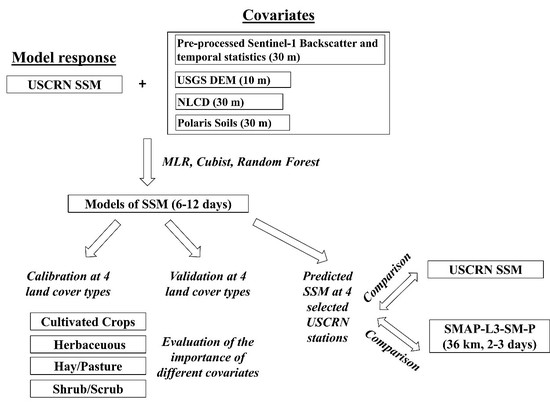
To retrieve surface soil moisture (SSM) (at the depth of 0–0.05 m) at the USCRN stations using Sentinel-1 data collected from 2016 to 2017 combined with ancillary data (e.g., terrain, land cover, soil properties), and to evaluate the model performance in 2018 for different land cover types and with different algorithms.
(2)
To evaluate the contribution of different ancillary variables for predicting soil moisture dynamics for future SSM retrieval across larger spatial extents.
Two hypotheses will be tested in the study: (1) SSM can be empirically retrieved at the USCRN stations in different land cover by combining Sentinel-1 with other ancillary data, and; (2) Sentinel-1 backscatter and ancillary data have different influences on the SSM model performance.

2. Materials and Methods

In this study, SSM retrieval models were established between the in-situ soil sensor SSM measurements (used as the model response), Sentinel-1 data, and various ancillary data (used as covariates). We describe these in turn below. Note that the acronyms are listed in Table A1.

2.1. U.S. Climate Reference Network SSM Database

In total, 66 USCRN sites were included for building the SSM retrieval models (Figure 1). Soil moisture sensors at the USCRN sites measure soil volumetric water content (VWC) at five depths (i.e., 0–0.05, 0.05–0.10, 0.10–0.20, 0.20–0.50, 0.50–1.00 m) every 30 min. We used the daily average VWC measured at 0–0.05 m to generate models of SSM, as the C-band SAR signal cannot penetrate deeper into the surface of the soil except when there is a very dry soil surface [31].

2.2. Sentinel-1 Data

The Sentinel-1 satellites are C-band dual-polarization Synthetic Aperture Radars (SAR). The Sentinel-1 mission comprises two identical spacecraft, Sentinel-1A (S-1A) and Sentinel-1B (S-1B) launched in 2014 and 2016, respectively. Depending on the number of satellites, the revisit time is every 6 (single satellite) or 12 (double satellites) days. The Sentinel-1 data used in this study were obtained from mid-March to mid-November across the USCRN from 2016 to 2018 to minimize the frozen ground period because of the insensitivity of radar backscatter data to soil moisture in frozen soil. Backscatter measurements were used that were available at two polarizations, VV (vertical transmit/vertical receive) and VV+VH (vertical transmit/horizontal receive). For brevity, we refer them to VV and VH modes. Both VV and VH data were used in the model because they have different sensitivity to SSM under different vegetation and land surface conditions [19].
The data used in this study were the Sentinel-1 Ground Range Detected (GRD) scenes in interferometric wide (IW) swath mode. The backscatter data were preprocessed using Google Earth Engine with thermal noise removal, radiometric calibration, and terrain correction [32]. Terrain correction was done using a 30-m SRTM digital elevation model. The processed backscatter data were available at a 10-m scale.
To remove the speckle effect of the backscatter data, we used an aggregation approach following [19] to resample the 10-m backscatter images to the 30-m scale. We describe this briefly here: First, dynamic masks were applied to the raw images to exclude the backscatter values larger than –5 dB and smaller than –20 dB for the VV mode and to exclude the backscatter values larger than –10 dB and smaller than –30 dB for the VH mode. The upper limits of the masks were determined according to Bauer-Marschallinger et al. and represented urban features [19]; the lower limits of the masks were determined empirically based on the distribution of backscatter data over the three years and represented the sensor’s noises. Second, the processed images were passed through a Gaussian filter with a 3 × 3 kernel ( 1 16 [ 1 2 1 2 4 2 1 2 1 ] ). Third, the filtered images at the 10-m scale were aggregated to the 30-m scale by the arithmetic mean. The aggregated backscatter will be used in this study for building the retrieval model for SSM across the USCRN stations.
We derived a number of indices from the aggregated backscatter data such as temporal mean and standard deviation (SD) of VV and VH backscatter and the ratios of the temporal SD to temporal mean. The VV and VH backscatter data were calculated pixel-wise at the 30-m sampling-scale from 2016 to 2018.

2.3. Ancillary Data

Different ancillary data were used to retrieve SSM in combination with Sentinel-1 data. These include land cover, terrain parameters, and soil properties. These datasets are shown in Table 1 and described below. Precipitation data were not used as covariates as they did not directly affect the relationship between SSM and backscatter data. Conventionally, precipitation measurements are used as quality control flags for the retrieving algorithms [16].

2.3.1. Land Cover

Land cover (LC) affects soil moisture [33]. The LC information was derived from the National Land Cover Database (https://www.mrlc.gov/data/type/land-cover) which provides 30-m land cover across the USA in the year of 2016 [34]. The land cover types include Developed, Water, Wetland, Shrub/Scrub, Herbaceous, Hay/Pasture, Forest and Cultivated Crops. We combined Shrub/Scrub and Dwarf scrub into Shrub/Scrub, and Deciduous Forest, Evergreen Forest, and Mixed Forest into Forest. We excluded Developed and Water, and Forest because the C-band Sentinel-1 data cannot penetrate the dense vegetation cover [35]. Wetland was also excluded. Four merged LC types were used as covariates: Cultivated Crops, Hay/Pasture, Herbaceous, and Shrub/Scrub. The final LC types are shown in Figure 1.

2.3.2. Terrain Parameters

The interaction between SSM and SAR backscatter measurements is affected by topography characteristics [36] and soil conditions such as ground roughness [16,21,37]. We used terrain parameters to model this relationship. The 10-m U.S. Geological Survey (USGS) National Digital Elevation Model (DEM) was used (www.nd.gov/gis). Slope, aspect, terrain ruggedness index (TRI), and topographic wetness index (TWI) were computed using the DEM data with the “terrain” function from the “raster” R package [38]. TRI and TWI are geo-morphometric parameters and have an impact on soil moisture distribution and dynamics [39,40]. Although these large-scale terrain parameters do not directly affect the backscattering behavior of the ground surface, we used them to model the spatial and temporal variations of soil VWC that were measured at the USCRN stations and were averaged daily assuming that surface soil water redistribution occurs due to topographic differences over this period.

2.3.3. Soil Properties

Soil properties influence soil moisture dynamics across the spatial and temporal scale. The Probabilistic Remapping of Soil Survey Geographic (POLARIS) dataset was used [41]. The POLARIS provides a 30-m probabilistic estimation of soil properties at six different depths across the USA, which are spatially continuous and internally consistent. The mean values of estimated properties at 0–0.05 m, including bulk density (BD), sand, silt and clay contents, and soil organic matter (SOM) content were used as covariates in the empirical models given their role in controlling of soil moisture storage [42].
To extract the Sentinel-1 and ancillary data to the USCRN stations for establishing SSM retrieval models and for mapping the SSM across the field, approximately 10 × 10 km regions of interest (ROIs) were selected for all USCRN stations with the USCRN sensors located in the center of the ROIs as they were large enough to observe the soil water variation in different vegetation, terrain, and soil conditions. We cannot choose an ROI that is too large because the Sentinel-1 sensor cannot capture the regions within one day and the composite Sentinel-1 image does not represent SSM within a specific day. Sentinel-1 data, LC types, terrain parameters, and soil properties were extracted within these ROIs onto 30 × 30 m grids. Sentinel-1 data were aggregated onto the 30-m using the method described earlier. LC types and soil properties data had 30-m resolutions and did not require further manipulation. Terrain parameters were extracted onto the 30-m grid using the bilinear interpolation algorithm. Along with the measured soil VWC from the USCRN sensors, these ancillary data were compiled, extracted onto the USCRN measuring stations and used for establishing empirical models to retrieve SSM at the USCRN stations over three years.

2.4. Establishing Empirical SSM Retrieval Models

Once the SSM data were collected and Sentinel-1 and ancillary data were extracted onto the USCRN stations, three models were explored to establish SSM retrieval algorithms, including multiple linear regression, Cubist and the Random Forest models. The covariates of the models included the backscatter data (VV, VH, and angle) and temporal statistics (e.g., temporal mean and SD) of VV and VH, as well as other ancillary data such as terrain parameters, land cover, and soil properties (e.g., clay, silt, bulk density). We describe each of the models in turn. The overall flow chart of the methodology used in this study is shown in Figure 2.

2.4.1. MLR Model

A multiple linear regression (MLR) was built with data listed in Table 1. In brief, the model response was the SSM measured at the USCRN stations and the predictors included Sentinel-1 backscatter and incidence angle, soil properties (e.g., sand content), terrain parameters (e.g., slope), and land cover types. In this study, the Sentinel-1 data varied in space and time while soil properties, terrain parameters, and land cover types only varied in space. Here, we used backward elimination to select the predictors. Afterward, we fitted the model parameters using the ordinary least square algorithm.

2.4.2. Cubist Model

The cubist model is an M5 regression tree algorithm [43]. Regression tree algorithm yields rule-based models comprising one or more rules. For each rule there is a set of conditions related to a linear sub-model. It can explain the nonlinear relationship between target variables and independent variables [44,45]. Cubist models have been used previously for the estimation of soil moisture [46], precipitation [47], net ecosystem carbon exchange [48], percent land cover [45], and soil properties e.g., pH, organic carbon, total nitrogen and phosphorus, texture, depth, and clay content [49].
Similar to the MLR, a Cubist model was constructed to predict SSM measured at the USCRN using Sentinel-1 and other ancillary data as predictors (Table 1). We fitted 20 committee models for the optimal Cubist model to predict soil VWC. The mean values of the predictions from all the committee models were used to represent the final VWC. To fit the Cubist model, the “train” function from the R “caret” package was used to find the optimal model parameters [50].

2.4.3. Random Forest Model

Random Forest is a nonparametric algorithm based on similarities among observations to fit decision trees. To build a tree, a bootstrap sample (a random sample with replacement) is taken from observations. To determine a split at a node in a tree, a random subsample of predictor variables is taken to select the predictor that minimizes the regression error [51]. Nodes continue to be split until no further improvement in error is achieved. Omitted observations, termed the “out-of-bag” samples, are used to compute the regression errors for trees [51]. Random Forest has recently been widely applied to map various soil properties and water dynamics using remote sensing data (e.g., [52,53]).
Similar to MLR and Cubist, the Random Forest algorithm was used to fit SSM at the USCRN from a combination of Sentinel-1 data and other environmental covariates as predictors. The “train” function in the “caret” package in R software [50] was used to fit the Random Forest parameters. The number of resampling iterations, number of variables tried at each split, and number of trees were selected as 10, 11, and 500, respectively, for the optimum model selection after repeated 10-fold cross-validation.

2.4.4. Model Performance Analysis

To evaluate the model performance and the contribution of different controlling factors on SSM retrieval, we used the USCRN VWC measurements from 2016 to 2017 as the calibration dataset and VWC measurements in 2018 as the validation dataset. The coefficient of determination (R2), mean error (ME), and root mean square error (RMSE) were calculated for both calibration and validation datasets using the measured VWC at the USCRN stations and predicted VWC from different empirical SSM models.

2.4.5. SMAP Soil Moisture Product

To validate and compare the performance of three empirical SSM models, the NASA SMAP L3 SSM product was used (accessed from https://nsidc.org/data/smap/spl3smp/data-fields). The dataset was developed using physical models and was available at 36 km every 2–3 days. SMAP SSM data were extracted onto four selected locations representing different LC types (Figure 1).

3. Results

3.1. Performance of Different Models

3.1.1. Multiple Linear Regression

As shown in Table 2, the covariates selected in the MLR model can be divided into four categories, including backscatter and their temporal statistics (VV, VH, Mean of VV, Mean of VH, SD/Mean of VV), terrain parameters (slope, aspect, TPI, TRI, TWI), soil properties (BD, clay, silt), and LC types. It can be interpreted from Table 2 that all the covariates listed were significant at the 5% level of significance (p < 0.05) except for the Shrub/Scrub LC type. The overall MLR model was significant at the 5% level of significance. The MLR was moderately accurate (R2 = 0.556 and RMSE = 0.058 m3 m−3) for the calibration data (from 2016 to 2017). In terms of the validation datasets in 2018, the model had a moderate performance (R2 = 0.551 and RMSE = 0.059 m3 m−3) (Figure 3).
In the MLR model, the importance of different covariates can be evaluated based on the P values. As shown in Table 2, VV was the most significant covariate, followed by soil properties such as silt, clay, and LC type. By comparison, terrain parameters (e.g., aspect, TPI) were less important and angle was the least important covariate in the MLR model.

3.1.2. Cubist

In the Cubist model, four categories of covariates were used, including backscatter and their temporal statistics (VV, VH, Mean of VV, Mean of VH, SD/Mean of VV), terrain parameters (slope, aspect, TPI, TRI, TWI), soil properties (BD, clay, silt), and LC types. In total, 20 committees were fitted for the optimal Cubist model and each of the committees had several rule-based sub-models. For example, the first, second, and third committee had 27, 10, and 21 number of rules that were chosen for optimum model building inside the “caret” package in R. Each rule fitted a regression equation between VWC and other covariates based on the mean, range, and estimated error of selected covariates (e.g., sand, SOM, VV, VH). The coefficents of the regression equations were selected based on the weightage decided by the optimum model build inside the “caret” package in R. The summary of the Cubist model formula is shown in Appendix A (Figure A1).
In the Cubist model, different conditions and predictors were determined and indicate the covariate usage in the model. As shown in Table 3, SOM (57% of usage), silt (39%), sand (34%), clay (26%), SD of VV (18%), aspect (18%), VV (18%), VH (17%) and other covariates were used as the conditions for selecting the rules of the Cubist model, whereas VV (90% of usage), silt (76%), sand (68%), VH (58%), SOM (55%) and others were used as the optimum model predictors. The weightages of the conditions and optimum model predictors were decided by the optimum model build inside the “caret” package in R. In terms of the model performance, it was improved compared to the MLR with R2 = 0.810 and 0.682, and RMSE = 0.051 and 0.064 m3 m−3 for the calibration and validation, respectively (Figure 3).

3.1.3. Random Forest

The Random Forest was established with the same four categories of covariates as the MLR and Cubist model. The importance of the covariates is shown in Table 4. The most important covariates were silt (%IncNodePurity = 9.3%) and sand (6.2%), followed by VV backscatter measurements (4.2%), SOM (3.5%), VH (3.4%), incidence angle (2.9%), and other covariates.
In terms of the model performance, the Random Forest model had the largest R2 (0.941) and the smallest RMSE (0.029 m3 m−3) for the calibration data as compared to the MLR and Cubist model. In terms of the validation data, the model was not good compared to the Cubist (R2 = 0.676 and RMSE = 0.065 m3 m−3) (Figure 3). In this study, the optimal numbers of trees and other hyperparameters were chosen by the “train” function in the R “caret” package and the final optimal model had 500 trees. This suggested that the Random Forest model was over-fitted to the calibration data compared to the Cubist model.

3.2. Model Performance within Different LC Types

The SSM retrieval models had different performance within different LC types (Table 5). In terms of the MLR model, the coefficient of determination (R2) calculated between measured VWC and predicted VWC for calibration datasets was largest in Herbaceous areas (0.503), followed by Shrub/Scrub (0.351), Cultivated Crops (0.264), and Hay/Pasture (0.230). In terms of the validation dataset, the patterns were slightly different, whereby Cultivated Crops had the largest R2 (0.451), followed by Herbaceous (0.351), Shrub/Scrub (0.314), and Hay/Pasture (0.104). Note that Cultivated Crops and Herbaceous land cover types always outperformed the Shrub/Scrub and Hay/Pasture.
This was not the case for Cubist and Random Forest models. When these two models were used, the model performance was best within the Herbaceous, followed by Shrub/Scrub, Hay/Pasture, and Cultivated Crops, for calibration datasets and within Shrub/Scrub, followed by Herbaceous, Cultivated Crops, and Hay/Pasture for validation datasets.
In terms of the importance of the covariates, the temporal Mean of VV and VH backscatter data (Mean of VV, Mean of VH), soil texture, and aspect were important in all three models (Table 2, Table 3 and Table 4). This indicated that these factors had strong influences on SSM. The land cover type was only important in the MLR and Random Forest model. This was possible because the Cubist model used other continuous covariates (e.g. SOM, sand, silt, clay content, SD of VV, aspect) to define the conditions that performed better than the land cover type (Table 3).
The temporal variations of measured and predicted SSM using the Cubist model are plotted for different LC types at four USCRN stations over 2016–2018 (Figure 4). The measured SSM was collected from the ground soil moisture probes at the measuring stations. The predicted SSM values were extracted from the Cubist model on to the measuring stations. This type of comparison was similarly used by Bauer-Marschallinger et al. [19] and Das et al. [29] to evaluate the performance of the SSM retrieval models. The performance of the SSM retrieval models varied with the stations. In general, soil VWC was well predicted in 2018 using historical (2016–2017) Sentinel-1 data with ancillary data in stations with Shrub/Scrub (MS_Newton), Herbaceous (SD_Pierre), and Cultivated Crops (MO_Chillicothe). Soil VWC was poorly retrieved in Hay/Pasture (KY_Versailles).
To compare the empirical model with the SMAP products, SMAP L3 Radiometer SSM estimates were also extracted on to the USCRN stations assuming the 36-km pixel values represent SSM measured at the stations (Figure 4). In general, the SMAP products have a larger model error compared to the empirical model established using Sentinel-1 data at these four locations.

4. Discussion

4.1. Importance of Covariates on SSM Retrieval at USCRN Stations

Compared with other “black-box” models such as artificial neural networks used to retrieve SSM (e.g., [27]), the use of MLR, Cubist and Random Forest algorithms makes the empirical models relatively easy to interpret. They also illustrate the relative importance of the covariates for retrieving SSM. As shown in Table 2, Table 3 and Table 4, the SSM dynamics at the USCRN stations are influenced by backscatter data and environmental variables, including soil properties, LC, terrain parameters. Among the three models, backscatter data and soil properties are most important in retrieving SSM, followed by several terrain parameters, and then LC types.
This highlights the need for measurement of high-resolution backscatter data from SAR sensors, as well as the development of high-resolution maps of soil properties for the future improvement of SSM empirical or physical retrieval models. Besides, high-resolution digital elevation models are also important as aspect, TPI, and TRI were used in the conditions and model of the Cubist model and found to be significant in the MLR and Random Forest model.

4.2. Implications of the Empirical SSM Retrieval Models

The empirical models established in this study have several advantages. First, the Cubist model is more accurate than the SMAP Level 3 radiometer-based SSM product (a resolution of 36 km) at the selected USCRN stations, particularly within Shrub/Scrub, Herbaceous, and Cultivated Crops (Figure 4). This was most likely due to the use of fine-resolution environmental covariates as compared to the SMAP model [16].
Second, the MLR model was worse than the Cubist and Random Forest models because the simplicity of the MLR model cannot account for the complex relationship between VWC and microwave data. This suggests that non-linear models should be used to retrieve SSM using Sentinel-1 data and is consistent with the previous studies that use non-linear models for predicting SSM (e.g., [54,55,56]). The Random Forest model over-fits the calibration dataset, so it should be used with caution for the future development of SSM retrieval models.
Third, the Cubist model is simple as no detailed information such as the ground roughness, emissivity, and opacity of the vegetation are required unlike those used in the physical models (e.g., [16,21]). Instead, we only used environmental covariates (soil properties, land cover, terrain parameters) that have become available across large spatial extents from various sources of remote sensing and ancillary data. When historical SSM measurements are available from the ground monitoring networks, SSM dynamics can be retrieved using a combination of Sentinel-1 and ancillary data in the future under similar land surface conditions. Because these environmental covariates are widely available across the US and the world [57,58,59], it is worth further exploring this approach to a large spatial extent (across the US or globally) by including more SSM network measurements [9].

4.3. Limitations of the Empirical SSM Retrieval Models

There are a few limitations of the empirical models. First, the empirical model established in this study can only retrieve SSM well in three LC types (Shrub/Scrub, Herbaceous, and Cultivated Crops). Future work is required to establish SSM retrieval models in other LC types, such as Hay/Pasture and Forest. The effective measuring depth of C-band SAR is around 0.05 m, so it is possible to combine Sentinel-1 data with other microwave data, such as the radiometer of the SMAP mission [29] and AMSR2. In a similar study, Alexakis et al. showed that Sentinel-1 backscatter data can be combined with vegetation indices (e.g., NDVI) to estimate SSM using a non-linear approach such as an artificial neural network (ANN) [56].
Alternatively, active and passive remote sensing data could be used to retrieve soil moisture coupled with statistical, empirical, and backscattering models [60]. It is also possible to assimilate these microwave data with other remote sensing satellite products, including optical and thermal bands, such as LANDSAT and Sentinel-2 (e.g., [61]) and ECOSTRESS [62] satellites to better account for the differences in leaf area and land surface radiance due to the spatial-temporal variations in SSM. Alternatively, a physical model such as Water Cloud Model could be effectively used for SSM retrieval from Synthetic Aperture Radar (SAR) imagery [63]. It is also feasible to combine multi-sensor satellite data from microwave and optical sensors to retrieve SSM using a hybrid approach [64].
Second, to implement this SSM model for irrigation scheduling whereby SSM measurements from sparse soil moisture measurements are available in the field (e.g., [65]), process models are required to forecast soil water storage and movement within the root-zone (e.g., [66,67]). This can be achieved by assimilating VWC measurements at multiple depths from soil moisture probes with mechanistic models using ensemble Kalman filtering (e.g., [68,69]). Alternatively, empirical and mechanistic models may be used to obtain deeper-layer soil water content from the satellite-derived SSM measurements [70,71,72].
Lastly, the small-scale roughness element is often used to model the backscatter signal from microwave radar [21,37,73]. Because most DEM data has a limited resolution (10 m), it is also possible to include high-resolution tomography radar imaging for improved terrain delineation under certain regions [74]. To apply the SSM model across a larger spatial extent, it is worth exploring how to downscale the roughness parameters from coarse-resolution DEM for developing the soil water retrieval model.

5. Conclusions

Empirical models are established for predicting surface soil moisture (SSM, 0–0.05 m) in 2018 based on historical (2016–2017) Sentinel-1 and ancillary data at the U.S. Climate Reference Network soil moisture. Multiple linear regression (MLR), Cubist, and Random Forest models are compared to fit the models using 30-m Sentinel-1 data, a 10-m digital elevation model, 30-m Polaris soil property maps, and 30-m land cover maps of the USA.
The Cubist model is better than the MLR and Random Forest (R2 = 0.68 and RMSE = 0.06 m3 m−3 for validation). The Cubist model performs best in Shrub/Scrub, followed by Herbaceous and Cultivated Crops but poorly in Hay/Pasture and shows better performance than the SSM retrieved by SMAP Radiometer at the 36-km resolution at several USCRN stations due to the use of fine-resolution environmental covariates. The SSM model performance is mostly affected by backscatter data, soil properties and terrain parameters, followed by land cover types. This indicates the need to improve the spatial resolution and accuracy of these land surface parameter products at the regional and global scales.
Future work is required to improve the model performance by including more SSM measurements, assimilating Sentinel-1 data with other remote sensing products such as microwave (SMAP, AMSR2), optical and thermal (LANDSAT, Sentinel-2, ECOSTRESS) satellites as well as developing high-resolution topography maps.

Author Contributions

S.C. and J.H. designed the study for soil water retrieval. S.C. performed the analysis. S.C., J.H., and A.E.H. wrote the paper. All authors have read and agreed to the published version of the manuscript.

Acknowledgments

We acknowledge the United States Department of Agriculture Hatch multi-state research formula fund for providing support for the project. The first author acknowledges the Indian Council of Agricultural Research for granting study leave and providing financial support. We acknowledge the editors and three anonymous reviewers for providing constructive comments that have helped us improve the quality of the manuscript.

Conflicts of Interest

The authors declare no conflict of interest.

Appendix A

Table A1. List of acronyms used in the paper.
AcronymsFull Form
USCRNU.S. Climate Reference Network
S-1Sentinel-1
SARSynthetic Aperture Radar
VVVertical transmit/vertical receive
VHVertical transmit/horizontal receive
SMAPSoil Moisture Active Passive
AMSR2Advanced Microwave Scanning Radiometer 2
SSMSurface Soil Moisture
VWCVolumetric Water Content
LCLand Cover
ROIRegion of Interest
GRDGround Range Detected
SRTMShuttle Radar Topography Mission
DEMDigital Elevation Model
USGSU.S. Geological Survey
TRITerrain Ruggedness Index
TWITopographic Wetness Index
TPITopographic Position Index
NDVINormalized Difference Vegetation Index
POLARISProbabilistic Remapping of Soil Survey Geographic
SOMSoil Organic Matter
BDBulk Density
MLRMultiple Linear Regression
RFRandom Forest
ANNArtificial Neural Netwrok
SDStandard Deviation
MEMean Error
RMSERoot Mean Square Error
R2Coefficient of Determination
Figure A1. Summary of Cubist rules.
Remotesensing 12 01242 g0a1

References

  1. Dorigo, W.; de Jeu, R. Satellite soil moisture for advancing our understanding of earth system processes and climate change. Inter. J. Appl. Earth Obs. Geoinf. 2016, 48, 1–4. [Google Scholar] [CrossRef]
  2. Cui, Y.; Long, D.; Hong, Y.; Zeng, C.; Zhou, J.; Han, Z.; Liu, R.; Wan, W. Validation and reconstruction of FY-3B/MWRI soil moisture using an artificial neural network based on reconstructed MODIS optical products over the Tibetan Plateau. J. Hydrol. 2016, 543, 242–254. [Google Scholar] [CrossRef]
  3. Fang, B.; Lakshmi, V. Soil moisture at watershed scale: Remote sensing techniques. J. Hydrol. 2014, 516, 258–272. [Google Scholar] [CrossRef]
  4. Seneviratne, S.I.; Corti, T.; Davin, E.L.; Hirschi, M.; Jaeger, E.B.; Lehner, I.; Orlowsky, B.; Teuling, A.J. Investigating soil moisture–climate interactions in a changing climate: A review. Earth-Sci. Rev. 2010, 99, 125–161. [Google Scholar] [CrossRef]
  5. Walker, J.P. Estimating Soil Moisture Profile Dynamics from Near-Surface Soil Moisture Measurements and Standard Meteorological Data. Ph.D. Thesis, University of Newcastle, Newcastle, UK, 1999. [Google Scholar]
  6. Calamita, G.; Brocca, L.; Perrone, A.; Piscitelli, S.; Lapenna, V.; Melone, F.; Moramarco, T. Electrical resistivity and TDR methods for soil moisture estimation in central Italy test-sites. J. Hydrol. 2012, 454, 101–112. [Google Scholar] [CrossRef]
  7. Vereecken, H.; Huisman, J.A.; Pachepsky, Y.; Montzka, C.; Van Der Kruk, J.; Bogena, H.; Weihermüller, L.; Herbst, M.; Martinez, G.; Vanderborght, J. On the spatio-temporal dynamics of soil moisture at the field scale. J. Hydrol. 2014, 516, 76–96. [Google Scholar] [CrossRef]
  8. Quiring, S.M.; Ford, T.W.; Wang, J.K.; Khong, A.; Harris, E.; Lindgren, T.; Goldberg, D.W.; Li, Z. The North American soil moisture database: Development and applications. Bull. Am. Meteorol. Soc. 2016, 97, 1441–1459. [Google Scholar] [CrossRef]
  9. Dorigo, W.A.; Wagner, W.; Hohensinn, R.; Hahn, S.; Paulik, C.; Xaver, A.; Gruber, A.; Drusch, M.; Mecklenburg, S.; van Oevelen, P.; et al. The International Soil Moisture Network: A data hosting facility for global in situ soil moisture measurements. Hydrol. Earth Syst. Sci. 2011, 15, 1675–1698. [Google Scholar] [CrossRef] [Green Version]
  10. Al Bitar, A.; Leroux, D.; Kerr, Y.H.; Merlin, O.; Richaume, P.; Sahoo, A.; Wood, E.F. Evaluation of SMOS soil moisture products over continental US using the SCAN/SNOTEL network. IEEE Trans. Geosci. Remote Sens. 2012, 50, 1572–1586. [Google Scholar] [CrossRef] [Green Version]
  11. Ochsner, T.E.; Linde, E.; Haffner, M.; Dong, J. Mesoscale Soil Moisture Patterns Revealed Using a Sparse In Situ Network and Regression Kriging. Water Resour. Res. 2019, 55, 4785–4800. [Google Scholar] [CrossRef]
  12. Li, X.; Shao, M.; Zhao, C.; Liu, T.; Jia, X.; Ma, C. Regional spatial variability of root-zone soil moisture in arid regions and the driving factors—A case study of Xinjiang, China. Can. J. Soil Sci. 2019, 99, 277–291. [Google Scholar] [CrossRef]
  13. Wagner, W.; Dorigo, W.; de Jeu, R.; Fernandez, D.; Benveniste, J.; Haas, E.; Ertl, M. Fusion of active and passive microwave observations to create an essential climate variable data record on soil moisture. ISPRS Ann. 2012, 7, 315–321. [Google Scholar]
  14. Engman, E.T. Applications of microwave remote sensing of soil moisture for water resources and agriculture. Remote Sens. Environ. 1991, 35, 213–226. [Google Scholar] [CrossRef]
  15. Petropoulos, G.P.; Ireland, G.; Barrett, B. Surface soil moisture retrievals from remote sensing: Current status, products & future trends. Phys. Chem. Earth Parts A/B/C 2015, 83, 36–56. [Google Scholar]
  16. Entekhabi, D.; Njoku, E.G.; O’Neill, P.E.; Kellogg, K.H.; Crow, W.T.; Edelstein, W.N.; Entin, J.K.; Goodman, S.D.; Jackson, T.J.; Johnson, J.; et al. The soil moisture active passive (SMAP) mission. Proc. IEEE 2010, 98, 704–716. [Google Scholar] [CrossRef]
  17. Mecklenburg, S.; Drusch, M.; Kerr, Y.H.; Font, J.; Martin-Neira, M.; Delwart, S.; Buenadicha, G.; Reul, N.; Daganzo-Eusebio, E.; Oliva, R.; et al. ESA’s soil moisture and ocean salinity mission: Mission performance and operations. IEEE Trans. Geosci. Remote Sens. 2012, 50, 1354–1366. [Google Scholar] [CrossRef] [Green Version]
  18. Parinussa, R.M.; Holmes, T.R.; Wanders, N.; Dorigo, W.A.; de Jeu, R.A. A preliminary study toward consistent soil moisture from AMSR2. J. Hydrometeorol. 2015, 16, 932–947. [Google Scholar] [CrossRef]
  19. Bauer-Marschallinger, B.; Freeman, V.; Cao, S.; Paulik, C.; Schaufler, S.; Stachl, T.; Modanesi, S.; Massari, C.; Ciabatta, L.; Brocca, L.; et al. Toward global soil moisture monitoring with Sentinel-1: Harnessing assets and overcoming obstacles. IEEE Trans. Geosci. Remote Sens. 2018, 57, 520–539. [Google Scholar] [CrossRef]
  20. Vreugdenhil, M.; Dorigo, W.A.; Wagner, W.; De Jeu, R.A.; Hahn, S.; Van Marle, M.J. Analyzing the vegetation parameterization in the TU-Wien ASCAT soil moisture retrieval. IEEE Trans. Geosci. Remote Sens. 2016, 54, 3513–3531. [Google Scholar] [CrossRef]
  21. Chaubell, M.J.; Yueh, S.H.; Dunbar, R.S.; Colliander, A.; Chen, F.; Chan, S.K.; Entekhabi, D.; Bindlish, R.; O’Neill, P.E.; Asanuma, J.; et al. Improved SMAP Dual-Channel Algorithm for the Retrieval of Soil Moisture. IEEE Trans. Geosci. Remote Sens. 2020. [Google Scholar] [CrossRef]
  22. Thoma, D.P.; Moran, M.S.; Bryant, R.; Rahman, M.M.; Collins, C.H.; Keefer, T.O.; Noriega, R.; Osman, I.; Skrivin, S.M.; Tischler, M.A.; et al. Appropriate scale of soil moisture retrieval from high resolution radar imagery for bare and minimally vegetated soils. Remote Sens. Environ. 2008, 112, 403–414. [Google Scholar] [CrossRef]
  23. Santi, E.; Paloscia, S.; Pettinato, S.; Fontanelli, G. Application of artificial neural networks for the soil moisture retrieval from active and passive microwave spaceborne sensors. Int. J. Appl. Earth Obs. Geoinf. 2016, 48, 61–73. [Google Scholar] [CrossRef]
  24. Wang, L.; Qu, J.J. Satellite remote sensing applications for surface soil moisture monitoring: A review. Front. Earth Sci. China 2009, 3, 237–247. [Google Scholar] [CrossRef]
  25. García, M.; Riaño, D.; Chuvieco, E.; Salas, J.; Danson, F.M. Multispectral and LiDAR data fusion for fuel type mapping using Support Vector Machine and decision rules. Remote Sens. Environ. 2011, 115, 1369–1379. [Google Scholar] [CrossRef]
  26. Lievens, H.; Reichle, R.H.; Liu, Q.; De Lannoy, G.J.M.; Dunbar, R.S.; Kim, S.B.; Das, N.N.; Cosh, M.; Walker, J.P.; Wagner, W. Joint Sentinel-1 and SMAP data assimilation to improve soil moisture estimates. Geophys. Res. Lett. 2017, 44, 6145–6153. [Google Scholar] [CrossRef] [PubMed]
  27. Santi, E.; Paloscia, S.; Pettinato, S.; Brocca, L.; Ciabatta, L.; Entekhabi, D. On the synergy of SMAP, AMSR2 AND SENTINEL-1 for retrieving soil moisture. Int. J. Appl. Earth Obs. Geoinf. 2018, 65, 114–123. [Google Scholar] [CrossRef]
  28. Bauer-Marschallinger, B.; Paulik, C.; Hochstöger, S.; Mistelbauer, T.; Modanesi, S.; Ciabatta, L.; Massari, C.; Brocca, L.; Wagner, W. Soil moisture from fusion of scatterometer and SAR: Closing the scale gap with temporal filtering. Remote Sens. 2018, 10, 1030. [Google Scholar] [CrossRef] [Green Version]
  29. Das, N.N.; Entekhabi, D.; Dunbar, R.S.; Chaubell, M.J.; Colliander, A.; Yueh, S.; Jagdhuber, T.; Chen, F.; Crow, W.; O’Neill, P.E.; et al. The SMAP and Copernicus Sentinel 1A/B microwave active-passive high resolution surface soil moisture product. Remote Sens. Environ. 2019, 233, 111380. [Google Scholar] [CrossRef]
  30. Bell, J.E.; Palecki, M.A.; Baker, C.B.; Collins, W.G.; Lawrimore, J.H.; Leeper, R.D.; Hall, M.E.; Kochendorfer, J.; Meyers, T.P.; Wilson, T.; et al. US Climate Reference Network soil moisture and temperature observations. J. Hydrometeorol. 2013, 14, 977–988. [Google Scholar] [CrossRef]
  31. Paloscia, S.; Pettinato, S.; Santi, E.; Notarnicola, C.; Pasolli, L.; Reppucci, A. Soil moisture mapping using Sentinel-1 images: Algorithm and preliminary validation. Remote Sens. Environ. 2013, 134, 234–248. [Google Scholar] [CrossRef]
  32. Rabus, B.; Eineder, M.; Roth, A.; Bamler, R. The shuttle radar topography mission—A new class of digital elevation models acquired by spaceborne radar. ISPRS J. Photogramm. Remote Sens. 2003, 57, 241–262. [Google Scholar] [CrossRef]
  33. Jawson, S.D.; Niemann, J.D. Spatial patterns from EOF analysis of soil moisture at a large scale and their dependence on soil, land-use, and topographic properties. Adv. Water Resour. 2007, 30, 366–381. [Google Scholar] [CrossRef]
  34. Yang, L.; Jin, S.; Danielson, P.; Homer, C.; Gass, L.; Bender, S.M.; Case, A.; Costello, C.; Dewitz, J.; Fry, J.; et al. A new generation of the United States National Land Cover Database: Requirements, research priorities, design, and implementation strategies. ISPRS J. Photogramm. Remote Sens. 2018, 146, 108–123. [Google Scholar] [CrossRef]
  35. Verhegghen, A.; Eva, H.; Ceccherini, G.; Achard, F.; Gond, V.; Gourlet-Fleury, S.; Cerutti, P. The potential of Sentinel satellites for burnt area mapping and monitoring in the Congo Basin forests. Remote Sens. 2016, 8, 986. [Google Scholar] [CrossRef] [Green Version]
  36. Mohanty, B.P.; Skaggs, T.H. Spatio-temporal evolution and time-stable characteristics of soil moisture within remote sensing footprints with varying soil, slope, and vegetation. Adv. Water Resour. 2001, 24, 1051–1067. [Google Scholar] [CrossRef]
  37. Neelam, M.; Colliander, A.; Mohanty, B.P.; Cosh, M.H.; Misra, S.; Jackson, T.J. Multiscale Surface Roughness for Improved Soil Moisture Estimation. IEEE Trans. Geosci. Remote Sens. 2020. [Google Scholar] [CrossRef]
  38. Hijmans, R.J.; Van Etten, J.; Cheng, J.; Mattiuzzi, M.; Sumner, M.; Greenberg, J.A.; Lamigueiro, O.P.; Bevan, A.; Racine, E.B.; Shortridge, A.; et al. Package ‘raster’. Available online: https://cran.r-project.org/web/packages/raster/raster.pdf (accessed on 13 April 2020).
  39. Różycka, M.; Migoń, P.; Michniewicz, A. Topographic Wetness Index and Terrain Ruggedness Index in geomorphic characterisation of landslide terrains, on examples from the Sudetes, SW Poland. Z. für Geomorphol. Suppl. Issues 2017, 61, 61–80. [Google Scholar] [CrossRef] [Green Version]
  40. Raduła, M.W.; Szymura, T.H.; Szymura, M. Topographic wetness index explains soil moisture better than bioindication with Ellenberg’s indicator values. Ecol. Indic. 2018, 85, 172–179. [Google Scholar] [CrossRef]
  41. Chaney, N.W.; Minasny, B.; Herman, J.D.; Nauman, T.W.; Brungard, C.W.; Morgan, C.L.; McBratney, A.B.; Wood, E.F.; Yimam, Y. POLARIS soil properties: 30-m probabilistic maps of soil properties over the contiguous United States. Water Resour. Res. 2019, 55, 2916–2938. [Google Scholar] [CrossRef]
  42. Yost, J.L.; Hartemink, A.E. Effects of carbon on moisture storage in soils of the Wisconsin Central Sands, USA. Eur. J. Soil Sci. 2019, 70, 565–577. [Google Scholar] [CrossRef]
  43. Quinlan, J.R. Learning with continuous classes. In Proceedings of the 5th Australian Joint Conference on Artificial Intelligence, Hobart, Tasmania, 16–18 November 1992; World Scientific: Singapore, 1992; pp. 343–348. [Google Scholar]
  44. Yang, C.C.; Prasher, S.O.; Enright, P.; Madramootoo, C.; Burgess, M.; Goel, P.K.; Callum, I. Application of decision tree technology for image classification using remote sensing data. Agric. Syst. 2003, 76, 1101–1117. [Google Scholar] [CrossRef]
  45. Huang, C.; Townshend, J.R.G. A stepwise regression tree for nonlinear approximation: Applications to estimating subpixel land cover. Int. J. Remote Sens. 2003, 24, 75–90. [Google Scholar] [CrossRef]
  46. Morellos, A.; Pantazi, X.E.; Moshou, D.; Alexandridis, T.; Whetton, R.; Tziotzios, G.; Wiebensohn, J.; Bill, R.; Mouazen, A.M. Machine learning based prediction of soil total nitrogen, organic carbon and moisture content by using VIS-NIR spectroscopy. Biosyst. Eng. 2016, 152, 104–116. [Google Scholar] [CrossRef] [Green Version]
  47. Ma, Z.; Shi, Z.; Zhou, Y.; Xu, J.; Yu, W.; Yang, Y. A spatial data mining algorithm for downscaling TMPA 3B43 V7 data over the Qinghai–Tibet Plateau with the effects of systematic anomalies removed. Remote Sens. Environ. 2017, 200, 378–395. [Google Scholar] [CrossRef]
  48. Xiao, J.; Zhuang, Q.; Baldocchi, D.D.; Law, B.E.; Richardson, A.D.; Chen, J.; Oren, R.; Starr, G.; Noormets, A.; Ma, S.; et al. Estimation of net ecosystem carbon exchange for the conterminous United States by combining MODIS and AmeriFlux data. Agric. For. Meteorol. 2008, 148, 1827–1847. [Google Scholar] [CrossRef] [Green Version]
  49. Henderson, B.L.; Bui, E.N.; Moran, C.J.; Simon, D.A.P. Australia-wide predictions of soil properties using decision trees. Geoderma 2005, 124, 383–398. [Google Scholar] [CrossRef]
  50. Kuhn, M. A Short Introduction to the caret Package. Available online: https://mran.microsoft.com/snapshot/2015-03-04/web/packages/caret/vignettes/caret.pdf (accessed on 13 April 2020).
  51. Hastie, T.; Tibshirani, R.; Friedman, J. Random forests. In The Elements of Statistical Learning; Springer Science & Business Media: New York, NY, USA, 2009; pp. 587–604. [Google Scholar]
  52. Ramcharan, A.; Hengl, T.; Nauman, T.; Brungard, C.; Waltman, S.; Wills, S.; Thompson, J. Soil property and class maps of the conterminous United States at 100-meter spatial resolution. Soil Sci. Soc. Am. J. 2018, 82, 186–201. [Google Scholar] [CrossRef] [Green Version]
  53. Tyralis, H.; Papacharalampous, G.; Langousis, A. A brief review of random forests for water scientists and practitioners and their recent history in water resources. Water 2019, 11, 910. [Google Scholar] [CrossRef] [Green Version]
  54. Baghdadi, N.; Cresson, R.; El Hajj, M.; Ludwig, R.; La Jeunesse, I. Estimation of soil parameters over bare agriculture areas from C-band polarimetric SAR data using neural networks. Hydrol. Earth Syst. Sci. 2012, 16, 1607. [Google Scholar] [CrossRef] [Green Version]
  55. Pierdicca, N.; Pulvirenti, L.; Pace, G. A prototype software package to retrieve soil moisture from Sentinel-1 data by using a bayesian multitemporal algorithm. IEEE J. Appl. Earth Obs. Remote Sens. 2014, 7, 153–166. [Google Scholar] [CrossRef]
  56. Alexakis, D.; Mexis, F.D.; Vozinaki, A.E.; Daliakopoulos, I.; Tsanis, I. Soil moisture content estimation based on Sentinel-1 and auxiliary earth observation products. A hydrological approach. Sensors 2017, 17, 1455. [Google Scholar] [CrossRef] [PubMed] [Green Version]
  57. Reuter, H.I.; Nelson, A.; Jarvis, A. An evaluation of void-filling interpolation methods for SRTM data. Int. J. Geogr. Inf. Sci. 2007, 21, 983–1008. [Google Scholar] [CrossRef]
  58. Chen, J.; Chen, J.; Liao, A.; Cao, X.; Chen, L.; Chen, X.; He, C.; Han, G.; Peng, S.; Lu, M.; et al. Global land cover mapping at 30 m resolution: A POK-based operational approach. ISPRS J. Photogram. Remote Sens. 2015, 103, 7–27. [Google Scholar] [CrossRef] [Green Version]
  59. Hengl, T.; de Jesus, J.M.; Heuvelink, G.B.; Gonzalez, M.R.; Kilibarda, M.; Blagotić, A.; Shangguan, W.; Wright, M.N.; Geng, X.; Bauer-Marschallinger, B.; et al. SoilGrids250m: Global gridded soil information based on machine learning. PLoS ONE 2017, 12, e0169748. [Google Scholar] [CrossRef] [Green Version]
  60. Ahmed, A.; Zhang, Y.; Nichols, S. 2011. Review and evaluation of remote sensing methods for soil-moisture estimation. SPIE Rev. 2011, 2, 028001. [Google Scholar]
  61. Gao, Q.; Zribi, M.; Escorihuela, M.; Baghdadi, N. Synergetic use of Sentinel-1 and Sentinel-2 data for soil moisture mapping at 100 m resolution. Sensors 2017, 17, 1966. [Google Scholar] [CrossRef] [Green Version]
  62. Hulley, G.; Hook, S.; Fisher, J.; Lee, C. ECOSTRESS, A NASA Earth-Ventures Instrument for studying links between the water cycle and plant health over the diurnal cycle. In Proceedings of the 2017 IEEE International Geoscience and Remote Sensing Symposium (IGARSS), Fort Worth, TX, USA, 23–28 July 2017; pp. 5494–5496. [Google Scholar]
  63. Saradjian, M.R.; Hosseini, M. Soil moisture estimation by using multipolarization SAR image. Adv. Space Res. 2011, 48, 278–286. [Google Scholar] [CrossRef]
  64. Hosseini, M.; Saradjian, M.R. Soil moisture estimation based on integration of optical and SAR images. Can. J. Remote Sens. 2011, 37, 112. [Google Scholar] [CrossRef]
  65. Huang, J.; Hartemink, A.E.; Arriaga, F.; Chaney, N.W. Unraveling Location-specific and Time-dependent Interactions between Soil Water Content and Environmental Factors in Cropped Sandy Soils Using Sentinel-1 and Moisture Probes. J. Hydrol. 2019, 575, 780–793. [Google Scholar] [CrossRef]
  66. Liang, X.; Liakos, V.; Wendroth, O.; Vellidis, G. Scheduling irrigation using an approach based on the van Genuchten model. Agric. Water Manag. 2016, 176, 170–179. [Google Scholar] [CrossRef] [Green Version]
  67. Montzka, C.; Herbst, M.; Weihermüller, L.; Verhoef, A.; Vereecken, H. A global data set of soil hydraulic properties and sub-grid variability of soil water retention and hydraulic conductivity curves. Earth Syst. Sci. 2017, 9, 529–543. [Google Scholar] [CrossRef] [Green Version]
  68. Das, N.N.; Mohanty, B.P. Root zone soil moisture assessment using remote sensing and vadose zone modeling. Vadose Zone J. 2006, 5, 296–307. [Google Scholar] [CrossRef] [Green Version]
  69. Huang, J.; McBratney, A.B.; Minasny, B.; Triantafilis, J. Monitoring and modelling soil water dynamics using electromagnetic conductivity imaging and the ensemble Kalman filter. Geoderma 2017, 285, 76–93. [Google Scholar] [CrossRef]
  70. Wagner, W.; Lemoine, G.; Rott, H. A method for estimating soil moisture from ERS scatterometer and soil data. Remote Sens. Environ. 1999, 70, 191–207. [Google Scholar] [CrossRef]
  71. Albergel, C.; Rüdiger, C.; Pellarin, T.; Calvet, J.C.; Fritz, N.; Froissard, F.; Suquia, D.; Petitpa, A.; Piguet, B.; Martin, E. From near-surface to root-zone soil moisture using an exponential filter: An assessment of the method based on in-situ observations and model simulations. Hydrol. Earth Syst. Sci. 2008, 12, 1323–1337. [Google Scholar] [CrossRef] [Green Version]
  72. Sadeghi, M.; Ebtehaj, A.; Crow, W.T.; Gao, L.; Purdy, A.J.; Fisher, J.B.; Jones, S.B.; Babaeian, E.; Tuller, M. Global Estimates of Land Surface Water Fluxes from SMOS and SMAP Satellite Soil Moisture Data. J. Hydrometeorol. 2020, 21, 241–253. [Google Scholar] [CrossRef]
  73. Fung, A.K.; Liu, W.Y.; Chen, K.S.; Tsay, M.K. An improved IEM model for bistatic scattering from rough surfaces. J. Electromagn. Waves Appl. 2002, 16, 689–702. [Google Scholar] [CrossRef]
  74. Ludeno, G.; Catapano, I.; Renga, A.; Vetrella, A.R.; Fasano, G.; Soldovieri, F. Assessment of a micro-UAV system for microwave tomography radar imaging. Remote Sens. Environ. 2018, 212, 90–102. [Google Scholar] [CrossRef]
Figure 1. The U.S. Climate Reference Network (USCRN) stations used to retrieve surface soil moisture. The land cover map is obtained from the National Land Cover Database (https://www.mrlc.gov/data/type/land-cover). The red data points are the four USCRN stations of interest in this study.
Remotesensing 12 01242 g001
Figure 2. Block diagram of the method used in this study.
Remotesensing 12 01242 g002
Figure 3. Comparison of model performance based on the 66 U.S. Climate Reference Network stations over 2016–2018 for different machine learning algorithms including multiple linear regression model (a), Cubist model (c), and Random Forest (e) for the calibration dataset and multiple linear regression model (b), Cubist model (d), and Random Forest (f) for the validation dataset. Abbreviations: R2, coefficient of determination; RMSE, root mean square error (m3 m−3); ME, mean error (m3 m−3).
Remotesensing 12 01242 g003
Figure 4. Measured (black line) and predicted soil volumetric water content (VWC, m3 m−3) using the empirical model (red dots) and SMAP-L3-SM-P (blue dots) at four USCRN stations representing Cultivated Crops (MO_Chillicothe), Herbaceous (SD_Pierre), Hay/Pasture (KY_Versailles), and Shrub/Scrub (MS_Newton) during 2016–2018.
Remotesensing 12 01242 g004
Table 1. Remote sensing and environmental covariates used to retrieve soil moisture across the US.
DatasetsSpatial ResolutionTemporal ResolutionDepth (m)Comments
Soil water content measurements at the USCRNN.A.1-day0–0.05Empirical model response
ESA – Sentinel-1 backscatter measured at two polarizations (VV and VH) and incidence angle10 m6–12 days0–0.05Empirical model covariates
Land cover map from National Land Cover Dataset30 mN.A.Empirical model covariate
Terrain parameters from the USGS10 mN.A.Empirical model covariates
Soil property maps of the US (Polaris)30 mN.A.0–0.05Empirical model covariates
NASA-SMAP Level 3 radiometer-based surface soil moisture product36 km1-day0–0.05Independent validation dataset
Table 2. Multiple linear regression (MLR) model for retrieving soil volumetric water content (VWC, m3 m−3) at 0–0.05 m depth. Note: coefficient of determination, R2; VH, backscatter in vertical transmit/horizontal receive mode; VV, backscatter in vertical transmit/vertical receive mode; Mean of VV and VH refer to the temporal mean values of VV and VH backscatter measurements during the 2016–2018; TPI, topographic position index; BD, bulk density; and LC, land cover.
(a) Summary of fit
R20.556
R2 Adjusted0.554
Root mean square error0.078
No. of observations2,882
(b) Parameter estimates
CovariatesEstimateStandard Errort RatioProbability > |t|
Intercept0.1560.0227.072.0×10−12
VV0.0150.00115.382.0×10−51
angle0.0010.0002.628.8×10−3
Mean of VV−0.0230.002−11.324.0×10−29
Mean of VH0.0010.0015.836.3×10−9
aspect 0.0000.0108.321.0×10−16
TPI0.0540.0143.967.6×10−5
BD−0.0630.010−5.992.4×10−9
clay0.0040.00013.455×10−40
silt0.0020.00014.014×10−43
LC == Cultivated Crops0.0490.00412.334×10−34
LC == Herbaceous−0.0200.003−5.592.5×10−8
LC == Hay/Pasture0.0300.0038.956×10−19
LC == Shrub/Scrub−0.061
(c) Analysis of variance
SourceDegree of freedomSum of squares
Model1221.91
Error2,86917.50
Corrected total2,88139.41
F ratio299.40
Probability > F<0.0001
Table 3. Covariates usage in the Cubist model. Abbreviations: VH, backscatter measured in vertical transmit/horizontal receive mode; VV, backscatter measured in vertical transmit/vertical receive mode; Mean and SD of VV and VH refer to the temporal mean and temporal standard deviation values of VV and VH backscatter measurements during 2016–2018; TPI, topographic position index; TRI, terrain ruggedness index; TWI, topographic wetness index; BD, bulk density; SOM, soil organic matter; and LC, land cover.
CovariatesConditionsModel
SOM57%55%
silt39%76%
sand34%68%
clay26%44%
SD of VV18%47%
aspect18%30%
VV18%90%
VH17%58%
TPI15%25%
TWI11%28%
SD of VH10%45%
SD/Mean (VV)8%51%
Mean of VV8%39%
angle6%32%
slope5%38%
TRI3%29%
BD3%47%
Mean of VH3%31%
SD/Mean (VH)3%47%
Table 4. Covariates importance in the Random Forest model. Abbreviations: %IncNodePurity means a total decrease in node impurities from splitting on the variable, averaged over all trees; VH, backscatter measured in vertical transmit/horizontal receive mode; VV, backscatter measured in vertical transmit/vertical receive mode; Mean and SD of VV and VH refer to the temporal mean and temporal standard deviation values of VV and VH backscatter measurements during 2016–2018; TPI, topographic position index; TRI, terrain ruggedness index; TWI, topographic wetness index; BD, bulk density; SOM, soil organic matter; and LC, land cover.
Covariates%IncNodePurity
silt9.3
sand6.2
VV4.2
SOM3.5
VH3.4
angle2.9
LC1.6
clay1.0
aspect0.8
SD/Mean (VH)0.7
TPI0.7
BD0.5
Mean of VV0.4
SD of VV0.4
SD of VH0.4
SD/Mean (VV)0.4
slope0.4
Mean of VH0.3
TRI0.3
TWI0.3
Table 5. Model performance for different methods within different land cover types calculated for calibration and validation datasets. Abbreviations: N, number of samples; R2, coefficient of determination; RMSE, root mean square error (m3 m−3); ME, mean error (m3 m−3); RF, Random Forest.
CalibrationValidation
Cultivated CropsHay/PastureHerbaceousShrub/ScrubCultivated CropsHay/PastureHerbaceousShrub/Scrub
N303730934986210502550842
R2
MLR0.2640.2300.5030.3510.4510.1040.3510.314
Cubist0.5670.6710.8090.7230.5120.4570.5130.522
RF0.8950.9030.9430.9160.5090.3980.5230.543
RMSE
MLR0.0840.0920.0800.0590.0710.0980.0790.057
Cubist0.0620.0610.0490.0390.0670.0760.0720.048
RF0.0340.0360.0280.0230.0680.0800.0730.046
ME
MLR0.0000.0000.0000.0000.005−0.0080.005−0.000
Cubist−0.0010.001−0.001−0.003−0.000−0.0010.003−0.004
RF0.0000.045−0.000−0.0000.002−0.0010.0050.000

