Point Cloud Semantic Segmentation Using a Deep Learning Framework for Cultural Heritage

 ,
,  ,
,  , ,
, ,  ,
,  ,
,  and
and
Abstract
1. Introduction
2. State of the Art
2.1. Classification and Semantic Segmentation in the Field of Dch
2.2. Semantic Segmentation of Point Clouds
- Multiview-based: creation of a set of images from Point Clouds, on which ConvNets can be applied, having shown to achieve very high accuracy both in terms of classification and segmentation;
- Voxel-based: rasterization of Point Clouds in voxels, which allow to have an ordered grid of Point Clouds, while maintaining the continous properties and the third dimension, thus permitting the application of CNNs;
- Point-based: the classification and semantic segmentation are performed by applying features-based approaches; the DL has shown good results in numerous fields, but has not been applied to DCH oriented dataset yet.
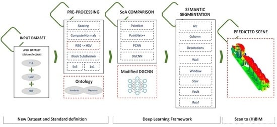
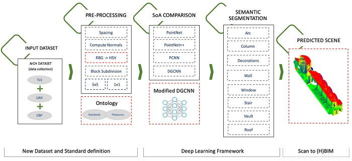
3. Materials and Methods
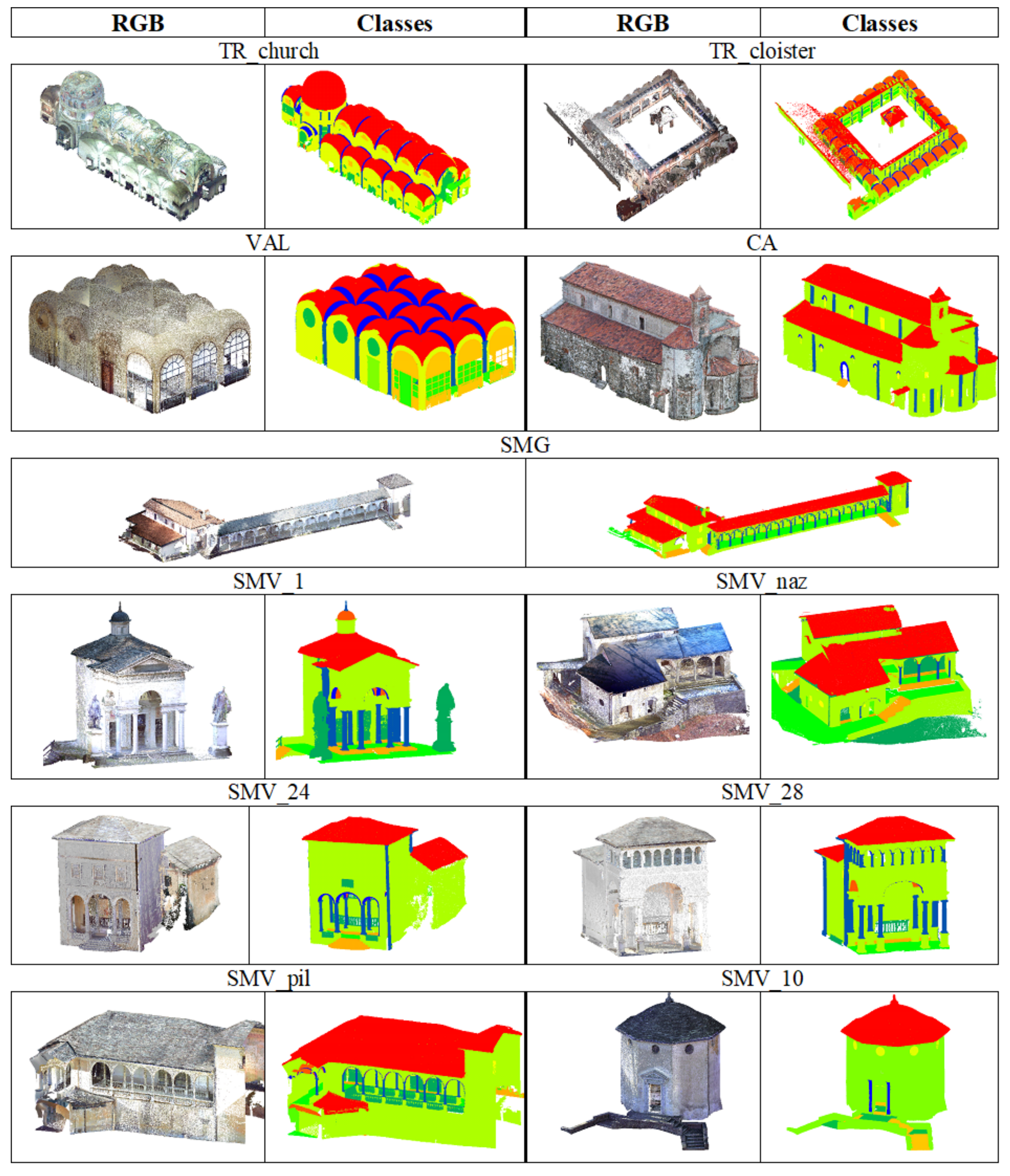
3.1. ArCH Dataset for Point Cloud Semantic Segmentation
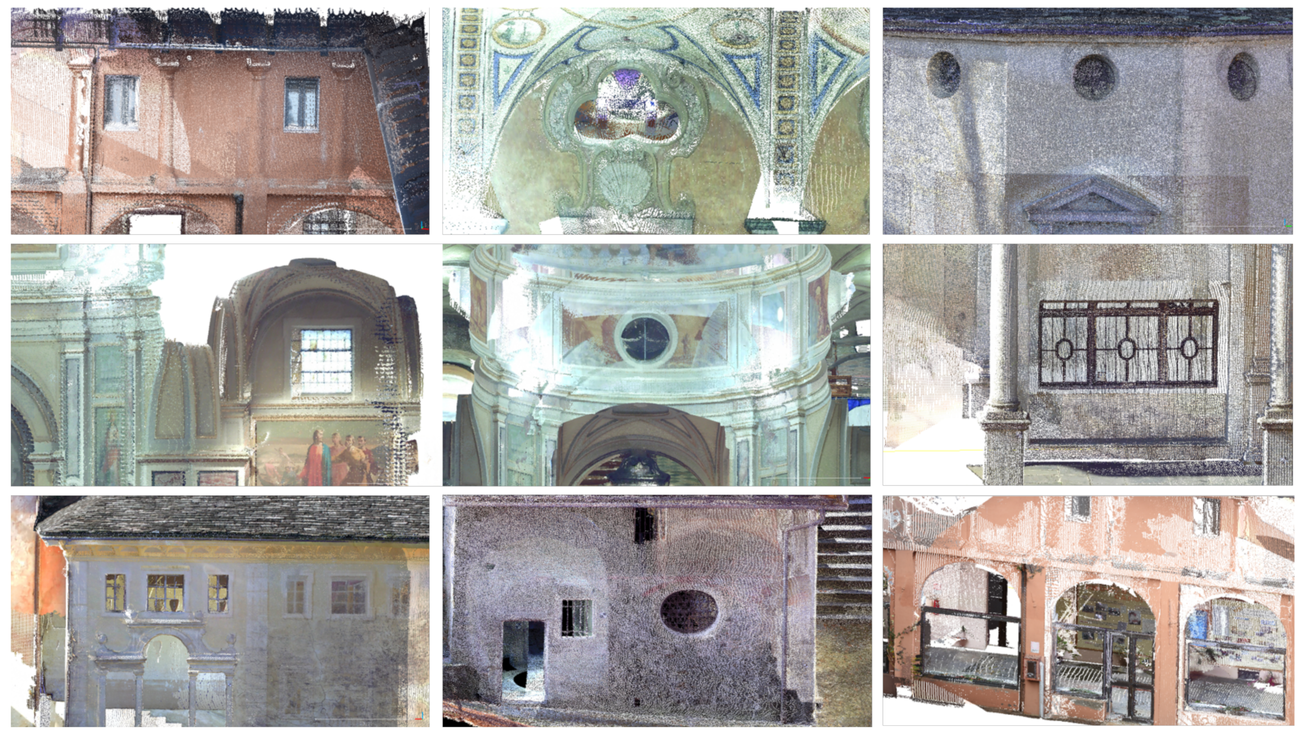
- The Sacri Monti (Sacred Mounts) of Ghiffa and Varallo. These two devotional complexes in northern Italy have been included in the UNESCO World Heritage List (WHL) in 2003. In the case of the Sacro Monte di Ghiffa, a 30 m loggia with tuscanic stone columns and half pilasters has been chosen; while for the Sacro Monte of Varallo 6 buildings have been included in the dataset, containing a total of 16 chapels, some of which very complex from an architectural point of view: barrel vaults, sometimes with lunettes, cross vaults, arcades, balustrades and so on.
- The Sanctuary of Trompone (TR). This is a wide complex dating back to the 16th century and it consists of a church (about 40 × 10 m) and a cloister (about 25 × 25 m), both included in the dataset. The internal structure of the church is composed of 3 naves covered by cross vaults supported in turn by stone columns. There is also a wide dome at the apse and a series of half-pilasters covering the sidewalls.
- The Church of Santo Stefano (CA) has a completely different compositional structure if compared with the previous one, being a small rural church from the 11th century. There is a stone masonry, not plastered, brick arches above the small windows and a series of Lombard band defining a decorated moulding under the tiled roof.
- The indoor scene of the Castello del Valentino (VA) is a courtly room part of an historical building recast from the 17th century. This hall is covered by cross vaults leaning on six sturdy breccia columns. Wide French windows illuminate the room and oval niches surrounded by decorative stuccoes are placed on the sidewalls. This case study is part of a serial site inserted in the WHL. of UNESCO in 1997.
3.2. Data Pre-Processing
3.3. Deep Learning for Point Cloud Semantic Segmentation
- PointNet [21], as it was the pioneer of this approach, obtaining permutation invariance of points by operating on each point independently and applying a symmetric function to accumulate features.
- its extensions PointNet++ [22] that analyzes neighborhoods of points in preference of acting on each separately, allowing the exploitation of local features even if with still some important limitations.
- PCNN [71], a DL framework for applying CNN to Point Clouds generalizing image CNNs. The extension and restriction operators are involved, permitting the use of volumetric functions associated to the Point Cloud.
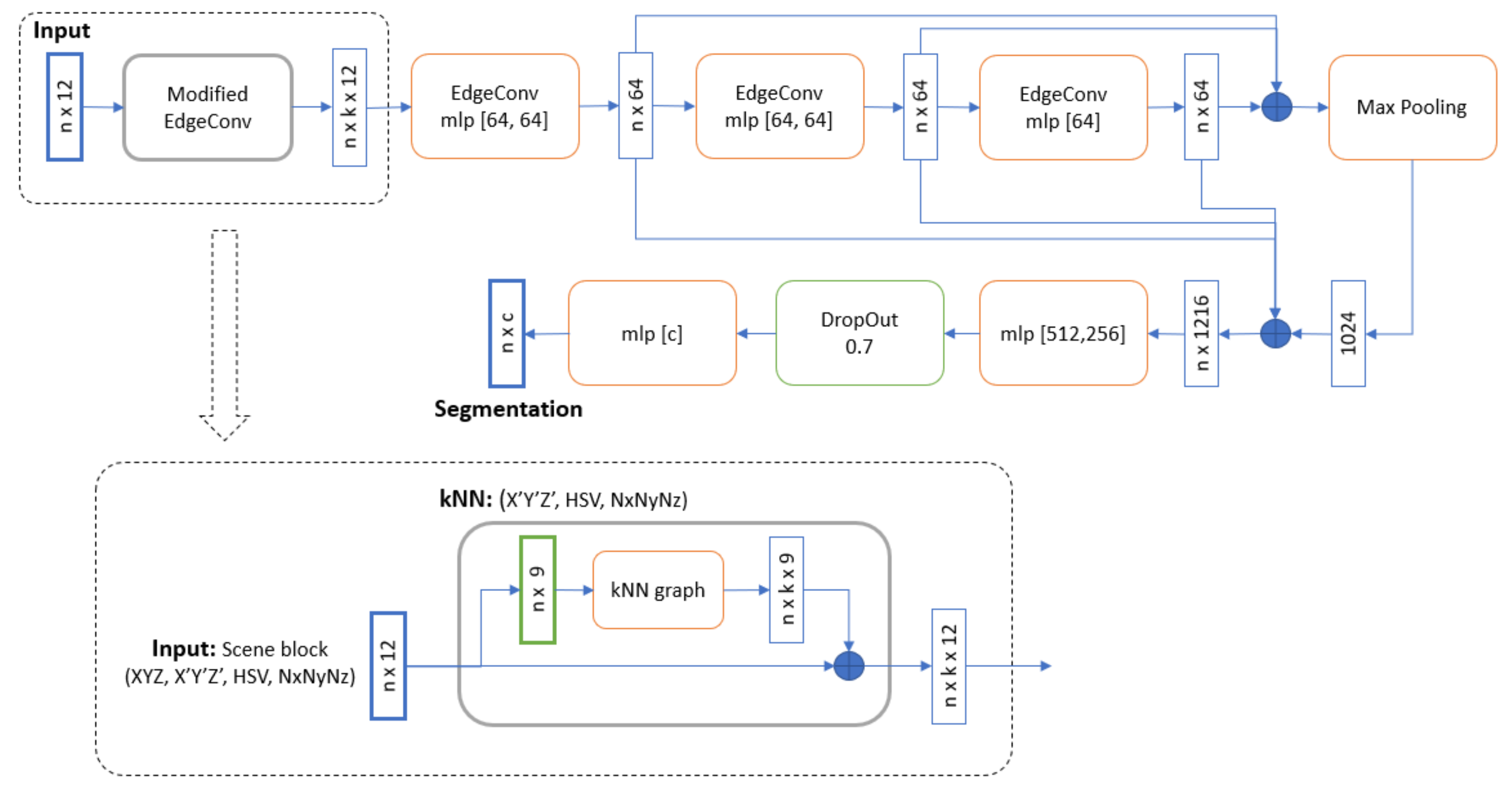
- DGCNN [32] that addresses these shortcomings by adding the EdgeConv operation. EdgeConv is a module that creates edge features describing the relationships between a point and its neighbors rather than generating point features directly from their embeddings. This module is permutation invariant and it is able to group points thanks to local graph, learning from the edges that link points.
3.4. DGCNN for DCH Point Cloud Dataset
4. Results
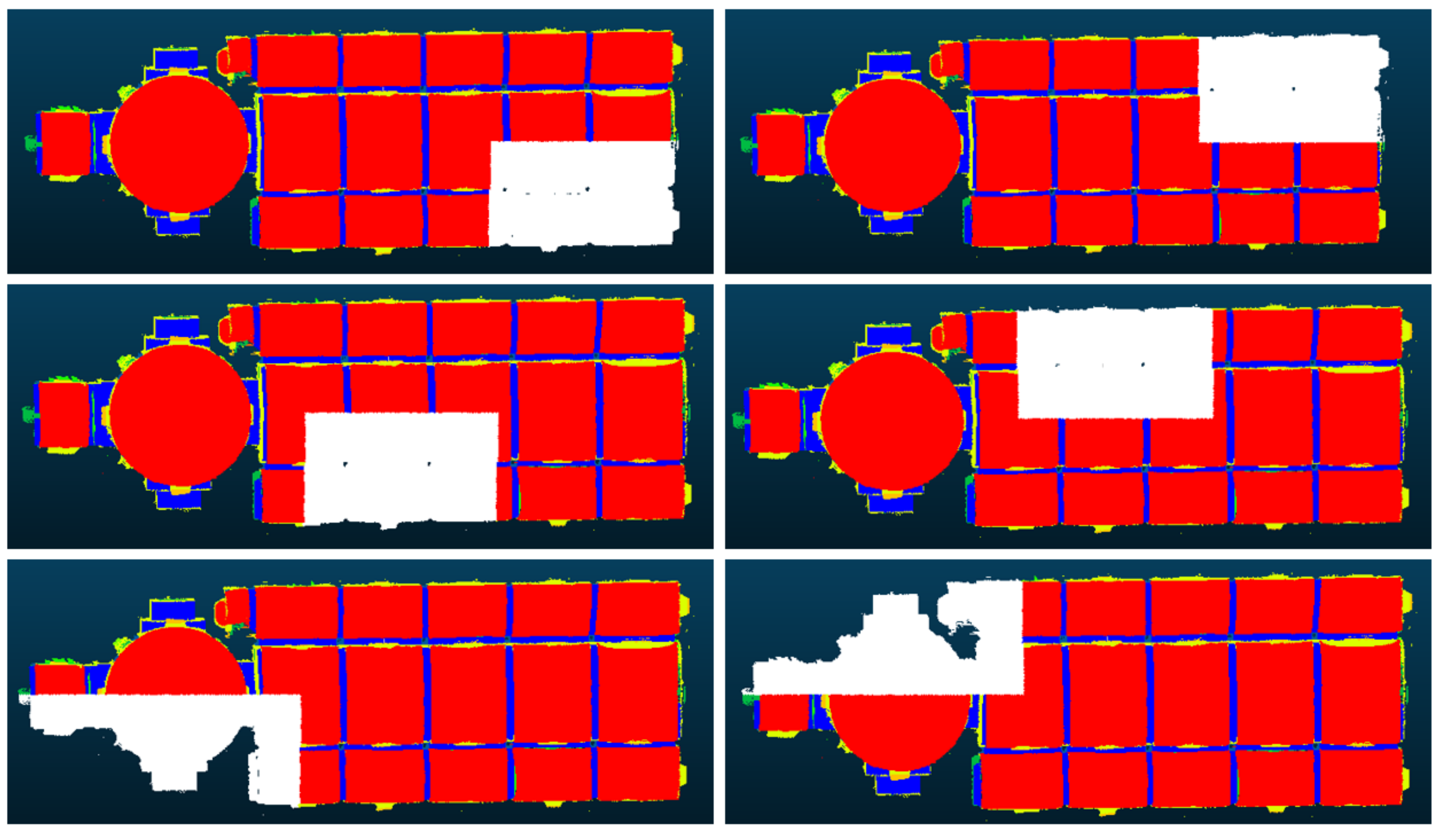
4.1. Segmentation of Partially Annotated Scene
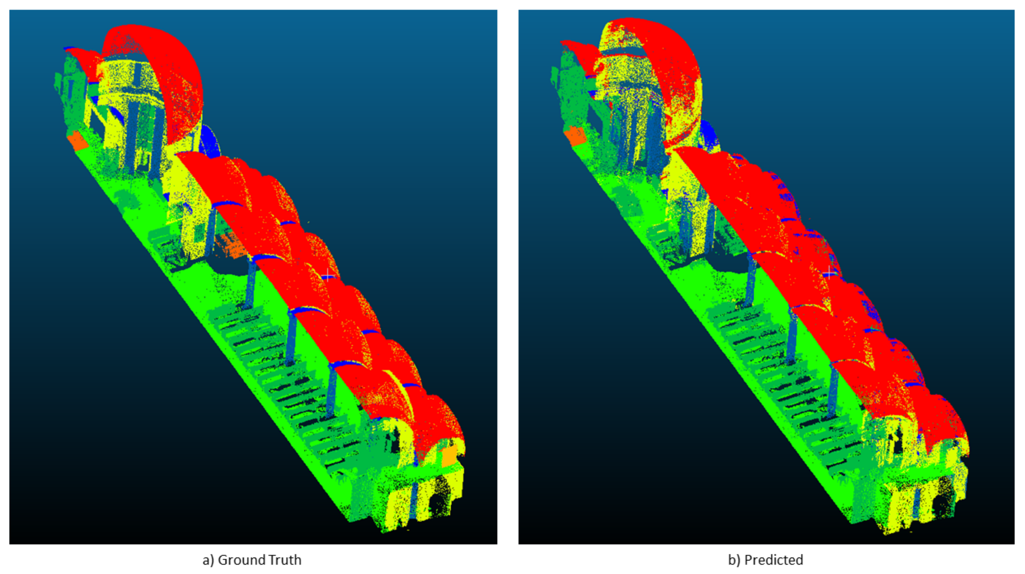
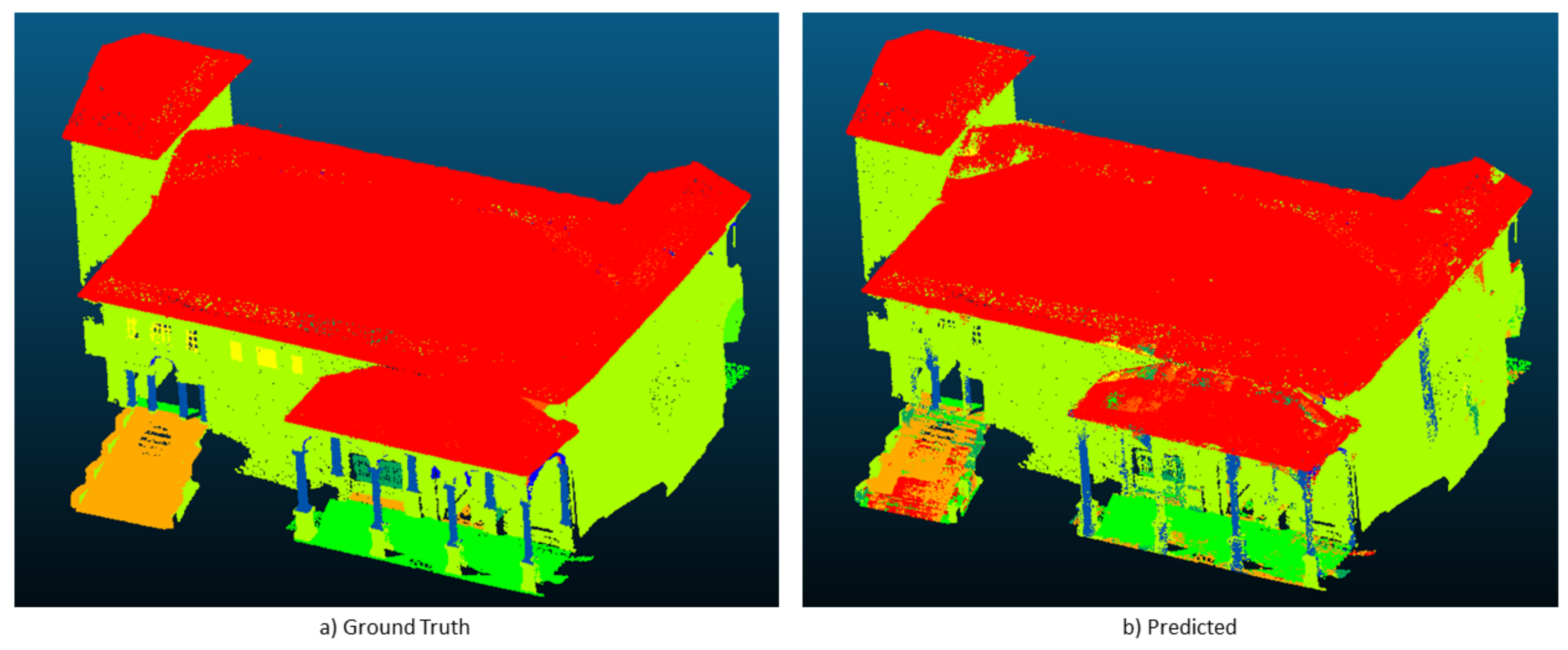
4.2. Segmentation of an Unseen Scene
5. Discussion
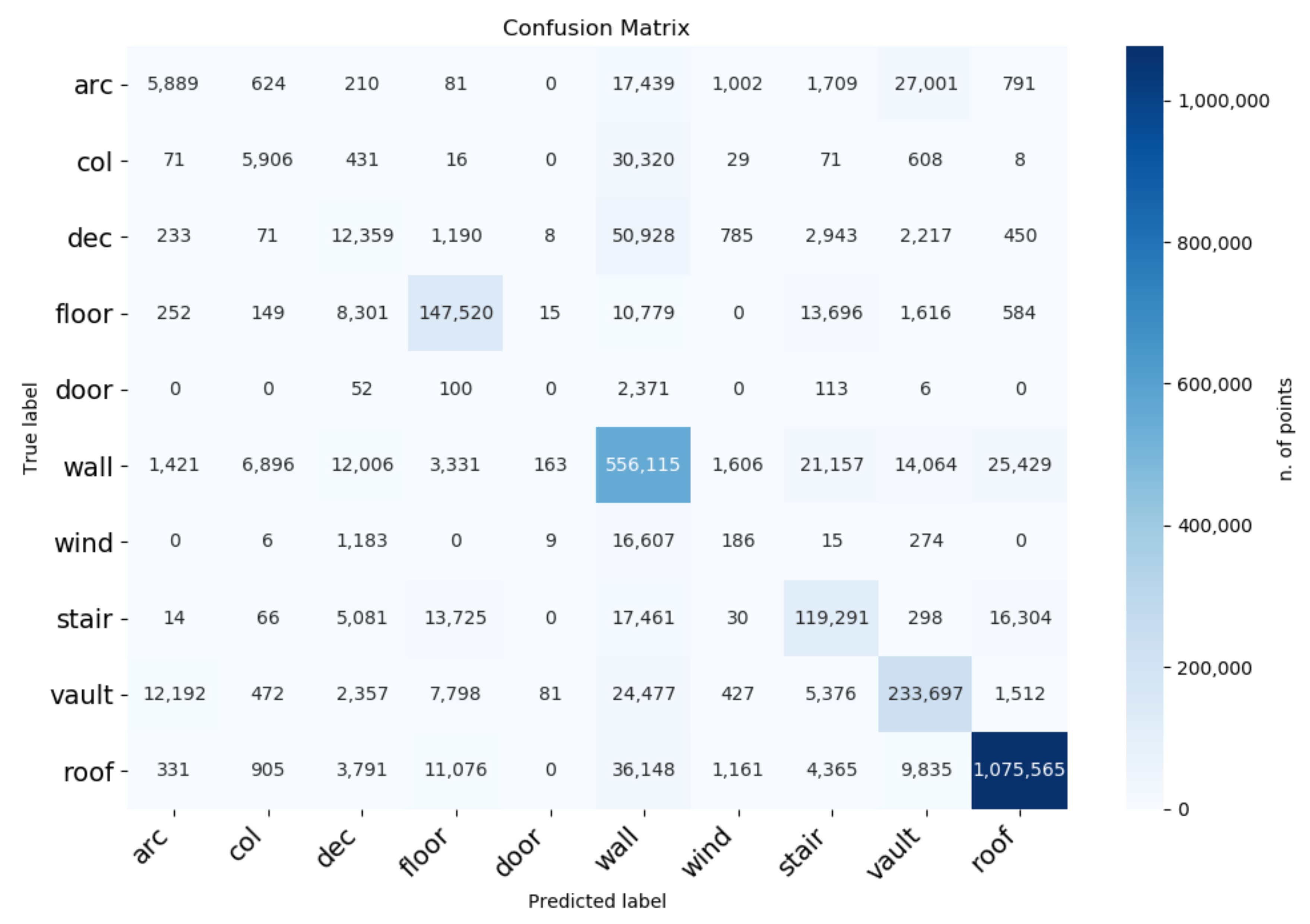
- Arc: the geometry of the elements of this class is very similar to that of the vaults and, although the dimensions of the arcs are not similar to the latter, most of the time they are really close to the vaults, almost a continuation of these elements. For these reasons the result is partly justifiable and could lead to the merging of these two classes.
- Dec: in this class, which can also be defined as “Others” or “Unassigned”, all the elements that are not part of the other classes (such as benches, paintings, confessionals…) are included. Therefore it is not fully considered among the results.
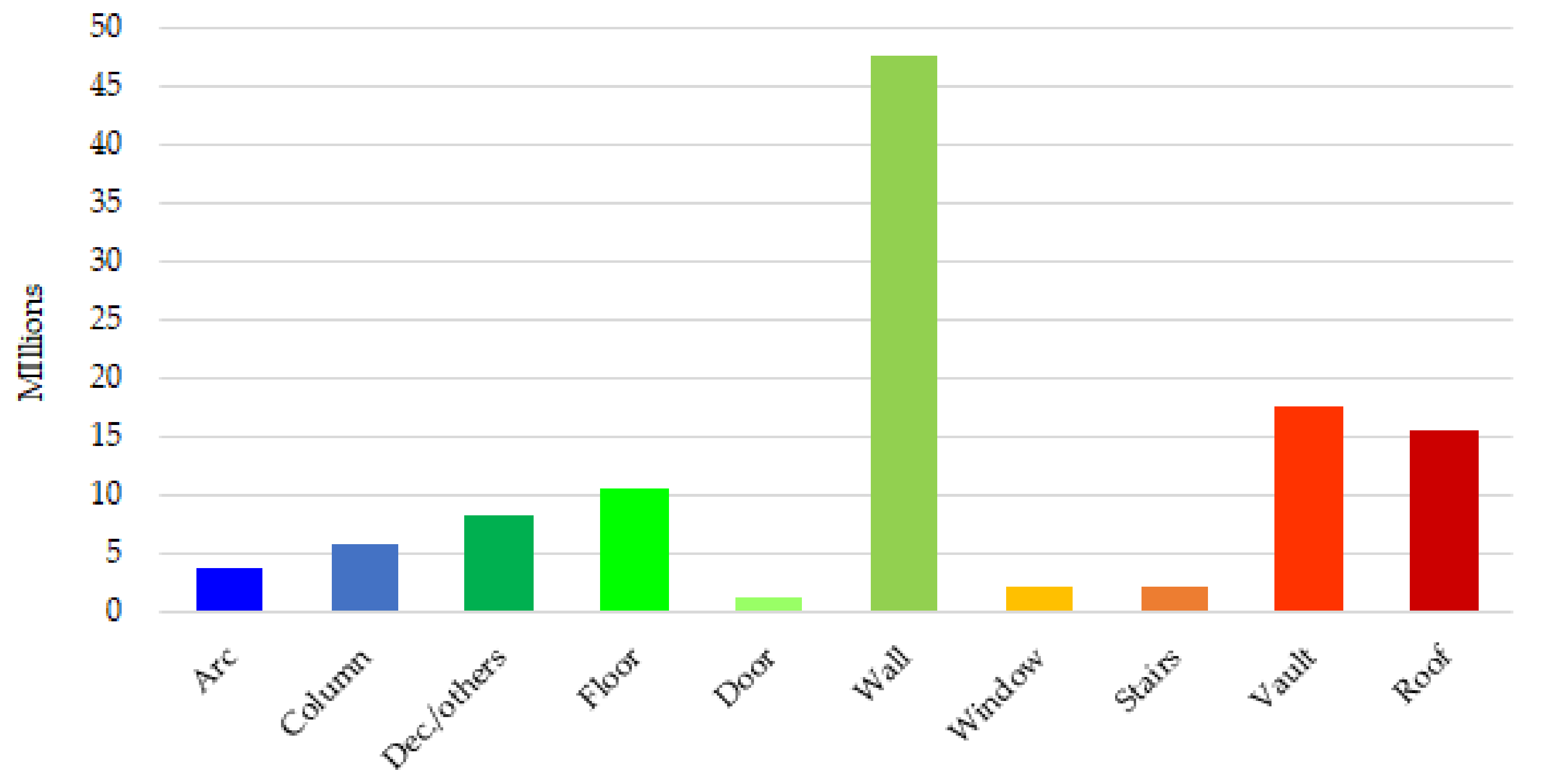
- Door: the null result is almost certainly due to the very low number of points present in this class (Figure 8). This is due to the fact that, in the proposed case studies of CH, it is more common to find large arches that mark the passage from one space to another and the doors are barely present. In addition, many times, the doors were open or with occlusions, generating a partial view and acquisition of these elements.
- Window: in this case the result is not due to the low number of windows present in the case study, but to the high heterogeneity between them. In fact, although the number of points in this class is greater, the shapes of the openings are very different from each other (three-foiled, circular, elliptical, square and rectangular) (Figure 9). Moreover, being mostly composed of glazed surfaces, these surfaces are not detected by the sensors involved such as the TLS, therefore, unlike the use of images, in this case the number of points useful to describe these elements is reduced.
6. Conclusions
Author Contributions
Funding
Acknowledgments
Conflicts of Interest
References
- Grilli, E.; Dininno, D.; Petrucci, G.; Remondino, F. From 2D to 3D supervised segmentation and classification for cultural heritage applications. Int. Arch. Photogramm. Remote Sens. Spat. Inf. Sci. 2018, 42, 399–406. [Google Scholar] [CrossRef]
- Masiero, A.; Fissore, F.; Guarnieri, A.; Pirotti, F.; Visintini, D.; Vettore, A. Performance Evaluation of Two Indoor Mapping Systems: Low-Cost UWB-Aided Photogrammetry and Backpack Laser Scanning. Appl. Sci. 2018, 8, 416. [Google Scholar] [CrossRef]
- Bronzino, G.; Grasso, N.; Matrone, F.; Osello, A.; Piras, M. Laser-Visual-Inertial Odometry based solution for 3D Heritage modeling: The sanctuary of the blessed Virgin of Trompone. Int. Arch. Photogramm. Remote Sens. Spat. Inf. Sci. 2019, 4215, 215–222. [Google Scholar] [CrossRef]
- Barazzetti, L.; Banfi, F.; Brumana, R.; Oreni, D.; Previtali, M.; Roncoroni, F. HBIM and augmented information: Towards a wider user community of image and range-based reconstructions. In Proceedings of the 25th International CIPA Symposium 2015 on the International Archives of the Photogrammetry, Remote Sensing and Spatial Information Sciences, Taipei, Taiwan, 31 August–4 September 2015; Volume XL-5/W7, pp. 35–42. [Google Scholar]
- Osello, A.; Lucibello, G.; Morgagni, F. HBIM and virtual tools: A new chance to preserve architectural heritage. Buildings 2018, 8, 12. [Google Scholar] [CrossRef]
- Balletti, C.; D’Agnano, F.; Guerra, F.; Vernier, P. From point cloud to digital fabrication: A tangible reconstruction of Ca’Venier dei Leoni, the Guggenheim Museum in Venice. ISPRS Ann. Photogramm. Remote Sens. Spat. Inf. Sci. 2016, 3, 43. [Google Scholar] [CrossRef]
- Bolognesi, C.; Garagnani, S. From a Point Cloud Survey to a mass 3D modelling: Renaissande HBIM in Poggio a Caiano. Int. Arch. Photogramm. Remote Sens. Spat. Inf. Sci. 2018, 42. [Google Scholar] [CrossRef]
- Chiabrando, F.; Sammartano, G.; Spanò, A. Historical buildings models and their handling via 3D survey: From points clouds to user-oriented HBIM. Int. Arch. Photogramm. Remote Sens. Spat. Inf. Sci. 2016, 41. [Google Scholar] [CrossRef]
- Fregonese, L.; Taffurelli, L.; Adami, A.; Chiarini, S.; Cremonesi, S.; Helder, J.; Spezzoni, A. Survey and modelling for the BIM of Basilica of San Marco in Venice. Int. Arch. Photogramm. Remote Sens. Spat. Inf. Sci. 2017, 42, 303. [Google Scholar] [CrossRef]
- Barazzetti, L.; Previtali, M. Vault Modeling with Neural Networks. In Proceedings of the 8th International Workshop on 3D Virtual Reconstruction and Visualization of Complex Architectures, 3D-ARCH 2019. Copernicus GmbH, Bergamo, Italy, 6–8 February 2019; Volume 42, pp. 81–86. [Google Scholar]
- Borin, P.; Cavazzini, F. Condition Assessment of RC Bridges. Integrating Machine Learning, Photogrammetry and BIM. Int. Arch. Photogramm. Remote Sens. Spat. Inf. Sci. 2019, 42. [Google Scholar] [CrossRef]
- Bruno, N.; Roncella, R. A restoration oriented HBIM system for Cultural Heritage documentation: The case study of Parma cathedral. Int. Arch. Photogramm. Remote Sens. Spat. Inf. Sci. 2018, 42. [Google Scholar] [CrossRef]
- Oreni, D.; Brumana, R.; Della Torre, S.; Banfi, F. Survey, HBIM and conservation plan of a monumental building damaged by earthquake. Int. Arch. Photogramm. Remote Sens. Spat. Inf. Sci. 2017, 42. [Google Scholar] [CrossRef]
- Bitelli, G.; Dellapasqua, M.; Girelli, V.; Sanchini, E.; Tini, M. 3D Geomatics Techniques for an integrated approach to Cultural Heritage knowledge: The case of San Michele in Acerboli’s Church in Santarcangelo di Romagna. Int. Arch. Photogramm. Remote Sens. Spat. Inf. Sci. 2017, 42. [Google Scholar] [CrossRef]
- Quattrini, R.; Pierdicca, R.; Morbidoni, C. Knowledge-based data enrichment for HBIM: Exploring high-quality models using the semantic-web. J. Cult. Herit. 2017, 28, 129–139. [Google Scholar] [CrossRef]
- Capone, M.; Lanzara, E. Scan-to-BIM vs 3D ideal model HBIM: Parametric tools to study domes geometry. Int. Arch. Photogramm. Remote Sens. Spat. Inf. Sci. 2019, 42. [Google Scholar] [CrossRef]
- Murtiyoso, A.; Grussenmeyer, P. Point Cloud Segmentation and Semantic Annotation Aided by GIS Data for Heritage Complexes. In Proceedings of the 8th International Workshop 3D-ARCH “3D Virtual Reconstruction and Visualization of Complex Architecture”, Bergamo, Italy, 6–8 February 2019; pp. 523–528. [Google Scholar]
- Murtiyoso, A.; Grussenmeyer, P. Automatic Heritage Building Point Cloud Segmentation and Classification Using Geometrical Rules. Int. Arch. Photogramm. Remote Sens. Spat. Inf. Sci. 2019, 42. [Google Scholar] [CrossRef]
- Grilli, E.; Özdemir, E.; Remondino, F. Application of Machine and Deep Learning strategies for the classification of Heritage Point Clouds. Int. Arch. Photogramm. Remote Sens. Spat. Inf. Sci. 2019, 42. [Google Scholar] [CrossRef]
- Spina, S.; Debattista, K.; Bugeja, K.; Chalmers, A. Point cloud segmentation for cultural heritage sites. In Proceedings of the 12th International conference on Virtual Reality, Archaeology and Cultural Heritage, Prato, Italy, 18–21 October 2011; pp. 41–48. [Google Scholar]
- Qi, C.R.; Su, H.; Mo, K.; Guibas, L.J. Pointnet: Deep learning on point sets for 3d classification and segmentation. In Proceedings of the IEEE Conference on Computer Vision and Pattern Recognition, Honolulu, HI, USA, 21–26 July 2017; pp. 652–660. [Google Scholar]
- Qi, C.R.; Yi, L.; Su, H.; Guibas, L.J. Pointnet++: Deep hierarchical feature learning on point sets in a metric space. Advances in Neural Information Processing Systems. arXiv 2017, arXiv:1706.02413. [Google Scholar]
- Wang, W.; Yu, R.; Huang, Q.; Neumann, U. Sgpn: Similarity group proposal network for 3d point cloud instance segmentation. In Proceedings of the IEEE Conference on Computer Vision and Pattern Recognition, Salt Lake City, UT, USA, 18–23 June 2018; pp. 2569–2578. [Google Scholar]
- Zhang, K.; Hao, M.; Wang, J.; de Silva, C.W.; Fu, C. Linked Dynamic Graph CNN: Learning on Point Cloud via Linking Hierarchical Features. arXiv 2019, arXiv:1904.10014. [Google Scholar]
- Song, S.; Xiao, J. Sliding shapes for 3d object detection in depth images. In Proceedings of the ECCV 2014, European Conference on Computer Vision, Zurich, Switzerland, 6–12 September 2014; Springer: Berlin, Germany, 2014; pp. 634–651. [Google Scholar]
- Song, S.; Xiao, J. Deep sliding shapes for amodal 3d object detection in rgb-d images. In Proceedings of the IEEE Conference on Computer Vision and Pattern Recognition, Las Vegas, NV, USA, 26 June–1 July 2016; pp. 808–816. [Google Scholar]
- Ma, L.; Liu, Y.; Zhang, X.; Ye, Y.; Yin, G.; Johnson, B.A. Deep learning in remote sensing applications: A meta-analysis and review. ISPRS J. Photogramm. Remote Sens. 2019, 152, 166–177. [Google Scholar] [CrossRef]
- Tang, P.; Huber, D.; Akinci, B.; Lipman, R.; Lytle, A. Automatic reconstruction of as-built building information models from laser-scanned point clouds: A review of related techniques. Autom. Constr. 2010, 19, 829–843. [Google Scholar] [CrossRef]
- Tamke, M.; Evers, H.L.; Zwierzycki, M.; Wessel, R.; Ochmann, S.; Vock, R.; Klein, R. An Automated Approach to the Generation of Structured Building Information Models from Unstructured 3d Point Cloud Scans. In Proceedings of the IASS Annual Symposia. International Association for Shell and Spatial Structures (IASS), Tokio, Japan, 26–30 September 2016; Volume 2016, pp. 1–10. [Google Scholar]
- Macher, H.; Landes, T.; Grussenmeyer, P. From point clouds to building information models: 3D semi-automatic reconstruction of indoors of existing buildings. Appl. Sci. 2017, 7, 1030. [Google Scholar] [CrossRef]
- Thomson, C.; Boehm, J. Automatic geometry generation from point clouds for BIM. Remote Sens. 2015, 7, 11753–11775. [Google Scholar] [CrossRef]
- Wang, Y.; Sun, Y.; Liu, Z.; Sarma, S.E.; Bronstein, M.M.; Solomon, J.M. Dynamic graph cnn for learning on point clouds. ACM Trans. Graph. TOG 2019, 38, 146. [Google Scholar] [CrossRef]
- Mathias, M.; Martinovic, A.; Weissenberg, J.; Haegler, S.; Van Gool, L. Automatic architectural style recognition. ISPRS-Int. Arch. Photogramm. Remote Sens. Spat. Inf. Sci. 2011, 3816, 171–176. [Google Scholar] [CrossRef]
- Oses, N.; Dornaika, F.; Moujahid, A. Image-based delineation and classification of built heritage masonry. Remote Sens. 2014, 6, 1863–1889. [Google Scholar] [CrossRef]
- Stathopoulou, E.; Remondino, F. Semantic photogrammetry: Boosting image-based 3D reconstruction with semantic labeling. Int. Arch. Photogramm. Remote Sens. Spat. Inf. Sci. 2019, 42. [Google Scholar] [CrossRef]
- Llamas, J.; M Lerones, P.; Medina, R.; Zalama, E.; Gómez-García-Bermejo, J. Classification of architectural heritage images using deep learning techniques. Appl. Sci. 2017, 7, 992. [Google Scholar] [CrossRef]
- Grilli, E.; Remondino, F. Classification of 3D Digital Heritage. Remote Sens. 2019, 11, 847. [Google Scholar] [CrossRef]
- Barsanti, S.G.; Guidi, G.; De Luca, L. Segmentation of 3D Models for Cultural Heritage Structural Analysis–Some Critical Issues. ISPRS Ann. Photogramm. Remote Sens. Spat. Inf. Sci. 2017, 4, 115. [Google Scholar] [CrossRef]
- Zaheer, M.; Kottur, S.; Ravanbakhsh, S.; Poczos, B.; Salakhutdinov, R.R.; Smola, A.J. Deep sets. Advances in Neural Information Processing Systems. arXiv 2017, arXiv:1703.06114. [Google Scholar]
- Weinmann, M.; Jutzi, B.; Hinz, S.; Mallet, C. Semantic point cloud interpretation based on optimal neighborhoods, relevant features and efficient classifiers. ISPRS J. Photogramm. Remote Sens. 2015, 105, 286–304. [Google Scholar] [CrossRef]
- Maturana, D.; Scherer, S. Voxnet: A 3d convolutional neural network for real-time object recognition. In Proceedings of the 2015 IEEE/RSJ International Conference on Intelligent Robots and Systems (IROS), Hamburg, Germany, 28 September–2 October 2015; pp. 922–928. [Google Scholar]
- Shi, S.; Wang, X.; Li, H. Pointrcnn: 3D object proposal generation and detection from point cloud. In Proceedings of the IEEE Conference on Computer Vision and Pattern Recognition, Lonch Beach, CA, USA, 26–20 June 2019; pp. 770–779. [Google Scholar]
- Zhou, Y.; Tuzel, O. Voxelnet: End-to-end learning for point cloud based 3d object detection. In Proceedings of the IEEE Conference on Computer Vision and Pattern Recognition, Salt Lake City, UT, USA, 18–23 June 2018; pp. 4490–4499. [Google Scholar]
- Zhang, R.; Li, G.; Li, M.; Wang, L. Fusion of images and point clouds for the semantic segmentation of large-scale 3D scenes based on deep learning. ISPRS J. Photogramm. Remote Sens. 2018, 143, 85–96. [Google Scholar] [CrossRef]
- Li, Y.; Wu, B.; Ge, X. Structural segmentation and classification of mobile laser scanning point clouds with large variations in point density. ISPRS J. Photogramm. Remote Sens. 2019, 153, 151–165. [Google Scholar] [CrossRef]
- Che, E.; Jung, J.; Olsen, M.J. Object recognition, segmentation, and classification of mobile laser scanning point clouds: A state of the art review. Sensors 2019, 19, 810. [Google Scholar] [CrossRef] [PubMed]
- Xie, Y.; Tian, J.; Zhu, X.X. A Review of Point Cloud Semantic Segmentation. arXiv 2019, arXiv:1908.08854. [Google Scholar]
- Boulch, A.; Le Saux, B.; Audebert, N. Unstructured Point Cloud Semantic Labeling Using Deep Segmentation Networks. 3DOR 2017, 2, 7. [Google Scholar]
- Boulch, A.; Guerry, J.; Le Saux, B.; Audebert, N. SnapNet: 3D point cloud semantic labeling with 2D deep segmentation networks. Comput. Graph. 2018, 71, 189–198. [Google Scholar] [CrossRef]
- Yavartanoo, M.; Kim, E.Y.; Lee, K.M. Spnet: Deep 3d object classification and retrieval using stereographic projection. In Asian Conference on Computer Vision; Springer: Berlin, German, 2018; pp. 691–706. [Google Scholar]
- Feng, Y.; Zhang, Z.; Zhao, X.; Ji, R.; Gao, Y. GVCNN: Group-view convolutional neural networks for 3D shape recognition. In Proceedings of the IEEE Conference on Computer Vision and Pattern Recognition, Salt Lake City, UT, USA, 18–23 June 2018; pp. 264–272. [Google Scholar]
- Zhao, R.; Pang, M.; Wang, J. Classifying airborne LiDAR point clouds via deep features learned by a multi-scale convolutional neural network. Int. J. Geogr. Inf. Sci. 2018, 32, 960–979. [Google Scholar] [CrossRef]
- Wu, Z.; Song, S.; Khosla, A.; Yu, F.; Zhang, L.; Tang, X.; Xiao, J. 3D shapenets: A deep representation for volumetric shapes. In Proceedings of the IEEE Conference on Computer Vision and Pattern Recognition, Boston, MA, USA, 7–12 June 2015; pp. 1912–1920. [Google Scholar]
- Wang, Z.; Lu, F. VoxSegNet: Volumetric CNNs for semantic part segmentation of 3D shapes. IEEE Trans. Vis. Comput. Graph. 2019. [Google Scholar] [CrossRef]
- Li, Y.; Bu, R.; Sun, M.; Wu, W.; Di, X.; Chen, B. Pointcnn: Convolution on x-transformed points. Advances in Neural Information Processing Systems. arXiv 2018, arXiv:1801.07791. [Google Scholar]
- Su, H.; Jampani, V.; Sun, D.; Maji, S.; Kalogerakis, E.; Yang, M.H.; Kautz, J. Splatnet: Sparse lattice networks for point cloud processing. In Proceedings of the IEEE Conference on Computer Vision and Pattern Recognition, Salt Lake City, UT, USA, 18–23 June 2018; pp. 2530–2539. [Google Scholar]
- Wu, W.; Qi, Z.; Fuxin, L. Pointconv: Deep convolutional networks on 3d point clouds. In Proceedings of the IEEE Conference on Computer Vision and Pattern Recognition, Long Beach, CA, USA, 16–20 June 2019; pp. 9621–9630. [Google Scholar]
- Klokov, R.; Lempitsky, V. Escape from cells: Deep kd-networks for the recognition of 3d point cloud models. In Proceedings of the IEEE International Conference on Computer Vision, Honolulu, HI, USA, 21–26 July 2017; pp. 863–872. [Google Scholar]
- Li, J.; Chen, B.M.; Hee Lee, G. So-net: Self-organizing network for point cloud analysis. In Proceedings of the IEEE conference on computer vision and pattern recognition, Salt Lake City, UT, USA, 18–23 June 2018; pp. 9397–9406. [Google Scholar]
- Zeng, W.; Gevers, T. 3DContextNet: Kd Tree Guided Hierarchical Learning of Point Clouds Using Local and Global Contextual Cues. In Proceedings of the European Conference on Computer Vision (ECCV), Munich, Germany, 8–14 September 2018; pp. 1–16. [Google Scholar]
- Roveri, R.; Rahmann, L.; Oztireli, C.; Gross, M. A network architecture for point cloud classification via automatic depth images generation. In Proceedings of the IEEE Conference on Computer Vision and Pattern Recognition, Salt Lake City, UT, USA, 18–23 June 2018; pp. 4176–4184. [Google Scholar]
- Landrieu, L.; Simonovsky, M. Large-scale point cloud semantic segmentation with superpoint graphs. In Proceedings of the IEEE Conference on Computer Vision and Pattern Recognition, Salt Lake City, UT, USA, 18–23 June 2018; pp. 4558–4567. [Google Scholar]
- Simonovsky, M.; Komodakis, N. Dynamic edge-conditioned filters in convolutional neural networks on graphs. In Proceedings of the IEEE Conference on Computer Vision and Pattern Recognition, Honolulu, HI, USA, 21–26 July 2017; pp. 3693–3702. [Google Scholar]
- Wang, L.; Huang, Y.; Hou, Y.; Zhang, S.; Shan, J. Graph Attention Convolution for Point Cloud Semantic Segmentation. In Proceedings of the IEEE Conference on Computer Vision and Pattern Recognition, Long Beach, CA, USA, 16–20 June 2019; pp. 10296–10305. [Google Scholar]
- Geiger, A.; Lenz, P.; Stiller, C.; Urtasun, R. Vision meets Robotics: The KITTI Dataset. Int. J. Robot. Res. IJRR 2013, 32, 1231–1237. [Google Scholar] [CrossRef]
- De Deuge, M.; Quadros, A.; Hung, C.; Douillard, B. Unsupervised feature learning for classification of outdoor 3D scans. In Proceedings of the Australasian Conference on Robitics and Automation, Sydney, Australia, 2–4 December 2013; Volume 2, p. 1. [Google Scholar]
- Hackel, T.; Savinov, N.; Ladicky, L.; Wegner, J.D.; Schindler, K.; Pollefeys, M. SEMANTIC3D.NET: A new large-scale point cloud classification benchmark. ISPRS Ann. Photogramm. Remote Sens. Spat. Inf. Sci. 2017, IV-1-W1, 91–98. [Google Scholar] [CrossRef]
- Armeni, I.; Sener, O.; Zamir, A.R.; Jiang, H.; Brilakis, I.; Fischer, M.; Savarese, S. 3d semantic parsing of large-scale indoor spaces. In Proceedings of the IEEE Conference on Computer Vision and Pattern Recognition, Las Vegas, NV, USA, 27–30 June 2016; pp. 1534–1543. [Google Scholar]
- Munoz, D.; Bagnell, J.A.; Vandapel, N.; Hebert, M. Contextual classification with functional max-margin markov networks. In Proceedings of the 2009 IEEE Conference on Computer Vision and Pattern Recognition, Miami, FL, USA, 20–26 June 2009; pp. 975–982. [Google Scholar]
- Hana, X.F.; Jin, J.S.; Xie, J.; Wang, M.J.; Jiang, W. A comprehensive review of 3d point cloud descriptors. arXiv 2018, arXiv:1802.02297. [Google Scholar]
- Atzmon, M.; Maron, H.; Lipman, Y. Point convolutional neural networks by extension operators. arXiv 2018, arXiv:1803.10091. [Google Scholar] [CrossRef]
- Sural, S.; Qian, G.; Pramanik, S. Segmentation and histogram generation using the HSV color space for image retrieval. In Proceedings of the International Conference on Image Processing, Rochester, NY, USA, 22–25 September 2002; Volume 2, p. II. [Google Scholar]
- Pierdicca, R.; Mameli, M.; Malinverni, E.S.; Paolanti, M.; Frontoni, E. Automatic Generation of Point Cloud Synthetic Dataset for Historical Building Representation. In International Conference on Augmented Reality, Virtual Reality and Computer Graphics; Springer: Berlin, Germany, 2019; pp. 203–219. [Google Scholar]
- Budden, D.; Fenn, S.; Mendes, A.; Chalup, S. Evaluation of colour models for computer vision using cluster validation techniques. In Robot Soccer World Cup; Springer: Berlin, Germany, 2012; pp. 261–272. [Google Scholar]
- Clini, P.; Quattrini, R.; Bonvini, P.; Nespeca, R.; Angeloni, R.; Mammoli, R.; Dragoni, A.F.; Morbidoni, C.; Sernani, P.; Mengoni, M.; et al. Digit(al)isation in Museums: Civitas Project—AR, VR, Multisensorial and Multiuser Experiences at the Urbino’s Ducal Palace. In Virtual and Augmented Reality in Education, Art, and Museums; IGI Global: Hershey, PA, USA, 2020; pp. 194–228. [Google Scholar] [CrossRef]


| Scene/Class | Arc | Column | Decoration | Floor | Door | Wall | Window | Stairs | Vault | Roof | TOTAL |
|---|---|---|---|---|---|---|---|---|---|---|---|
| 0 | 1 | 2 | 3 | 4 | 5 | 6 | 7 | 8 | 9 | ||
| TR_cloister | 900,403 | 955,791 | 765,864 | 1,948,029 | 779,019 | 10,962,235 | 863,792 | 2806 | 2,759,284 | 1,223,300 | 21,160,523 |
| TR_church_r | 466,472 | 658,100 | 1,967,398 | 1,221,331 | 85,001 | 3,387,149 | 145,177 | 84,118 | 2,366,115 | 0 | 10,380,861 |
| TR_church_l | 439,269 | 554,673 | 1,999,991 | 1,329,265 | 44,241 | 3,148,777 | 128,433 | 38,141 | 2,339,801 | 0 | 10,022,591 |
| VAL | 300,923 | 409,123 | 204,355 | 1,011,034 | 69,830 | 920,418 | 406,895 | 0 | 869,535 | 0 | 4,192,113 |
| CA | 17,299 | 172,044 | 0 | 0 | 30,208 | 3,068,802 | 33,780 | 11,181 | 0 | 1,559,138 | 4,892,452 |
| SMG | 309,496 | 1,131,090 | 915,282 | 1,609,202 | 18,736 | 7,187,003 | 137,954 | 478,627 | 2,085,185 | 7,671,775 | 21,544,350 |
| SMV_1 | 46,632 | 314,723 | 409,441 | 457,462 | 0 | 1,598,516 | 2011 | 274,163 | 122,522 | 620,550 | 3,846,020 |
| SMV_naz | 472,004 | 80,471 | 847,281 | 1,401,120 | 42,362 | 2,846,324 | 16,559 | 232,748 | 4,378,069 | 527,490 | 10,844,428 |
| SMV_24 | 146,104 | 406,065 | 154,634 | 20,085 | 469 | 366,2361 | 6742 | 131,137 | 305,086 | 159,480 | 4,992,163 |
| SMV_28 | 36,991 | 495,794 | 18,826 | 192,331 | 1,965,782 | 4481 | 13,734 | 184,261 | 197,679 | 3,109,879 | |
| SMV_pil | 584,981 | 595,117 | 1,025,534 | 1,146,079 | 26,081 | 7,358,536 | 313,925 | 811,724 | 2,081,080 | 3,059,959 | 17,003,016 |
| SMV_10 | 0 | 16,621 | 0 | 125,731 | 0 | 1,360,738 | 106,186 | 113,287 | 0 | 499,159 | 2,221,722 |
| TOTAL | 3,720,574 | 5,789,612 | 8,308,606 | 10,461,669 | 1,095,947 | 47,466,641 | 2,165,935 | 2,191,666 | 17,490,938 | 15,518,530 | 114,210,118 |
| Network | Features | Mean Acc. |
|---|---|---|
| DGCNN | XYZ + RGB | 0.897 |
| PointNet++ | XYZ | 0.543 |
| PointNet | XYZ | 0.459 |
| PCNN | XYZ | 0.742 |
| DGCNN-Mod | XYZ + Norm | 0.781 |
| Ours | XYZ + HSV + Norm | 0.918 |
| Network | Train Acc. | Valid Acc. | Test Acc. | Prec. | Rec. | F1-Score | Supp. |
|---|---|---|---|---|---|---|---|
| DGCNN | 0.993 | 0.799 | 0.733 | 0.721 | 0.733 | 0.707 | 1,437,696 |
| PointNet++ | 0.887 | 0.387 | 0.441 | 0.480 | 0.487 | 0.448 | 1,384,448 |
| PointNet | 0.890 | 0.320 | 0.307 | 0.405 | 0.306 | 0.287 | 1,335,622 |
| PCNN | 0.961 | 0.687 | 0.623 | 0.642 | 0.608 | 0.636 | 1,254,631 |
| Ours | 0.992 | 0.745 | 0.743 | 0.748 | 0.742 | 0.722 | 1,437,696 |
| Network | Metrics | Arc | Col | Dec | Floor | Door | Wall | Wind | Stair | Vault |
|---|---|---|---|---|---|---|---|---|---|---|
| DGCNN | Precision | 0.484 | 0.258 | 0.635 | 0.983 | 0.000 | 0.531 | 0.222 | 0.988 | 0.819 |
| Recall | 0.389 | 0.564 | 0.920 | 0.943 | 0.000 | 0.262 | 0.013 | 0.211 | 0.918 | |
| F1-Score | 0.431 | 0.354 | 0.751 | 0.963 | 0.000 | 0.351 | 0.024 | 0.348 | 0.865 | |
| Support | 69,611 | 36,802 | 240,806 | 287,064 | 8562 | 285,128 | 20,619 | 14,703 | 474,401 | |
| IoU | 0.275 | 0.215 | 0.602 | 0.929 | 0.000 | 0.213 | 0.012 | 0.210 | 0.764 | |
| PointNet++ | Precision | 0.000 | 0.000 | 0.301 | 0.717 | 0.000 | 0.531 | 0.000 | 0.000 | 0.654 |
| Recall | 0.000 | 0.000 | 0.792 | 0.430 | 0.000 | 0.284 | 0.000 | 0.000 | 0.765 | |
| F1-Score | 0.000 | 0.000 | 0.437 | 0.538 | 0.000 | 0.370 | 0.000 | 0.000 | 0.705 | |
| Support | 74,427 | 59,611 | 235,615 | 230,033 | 12,327 | 334,080 | 40,475 | 13,743 | 384,137 | |
| IoU | 0.000 | 0.000 | 0.311 | 0.409 | 0.000 | 0.215 | 0.000 | 0.000 | 0.681 | |
| PointNet | Precision | 0.000 | 0.000 | 0.155 | 0.588 | 0.000 | 0.424 | 0.175 | 0.000 | 0.600 |
| Recall | 0.000 | 0.000 | 0.916 | 0.422 | 0.000 | 0.078 | 0.004 | 0.000 | 0.387 | |
| F1-Score | 0.000 | 0.000 | 0.265 | 0.492 | 0.000 | 0.132 | 0.008 | 0.000 | 0.470 | |
| Support | 30,646 | 11,020 | 29,962 | 43,947 | 1851 | 69,174 | 3212 | 1057 | 87,659 | |
| IoU | 0.000 | 0.000 | 0.213 | 0.406 | 0.000 | 0.051 | 0.003 | 0.000 | 0.311 | |
| PCNN | Precision | 0.426 | 0.214 | 0.546 | 0.816 | 0.000 | 0.478 | 0.193 | 0.178 | 0.704 |
| Recall | 0.338 | 0.474 | 0.782 | 0.754 | 0.000 | 0.231 | 0.012 | 0.188 | 0.744 | |
| F1-Score | 0.349 | 0.294 | 0.608 | 0.809 | 0.000 | 0.281 | 0.021 | 0.306 | 0.779 | |
| Support | 65,231 | 32,138 | 220,776 | 212,554 | 8276 | 253,122 | 18,688 | 12,670 | 431,176 | |
| IoU | 0.298 | 0.273 | 0.592 | 0.722 | 0.000 | 0.210 | 0.010 | 0.172 | 0.703 | |
| Ours | Precision | 0.574 | 0.317 | 0.621 | 0.991 | 0.952 | 0.571 | 0.722 | 0.872 | 0.825 |
| Recall | 0.424 | 0.606 | 0.932 | 0.920 | 0.002 | 0.324 | 0.006 | 0.284 | 0.907 | |
| F1-Score | 0.488 | 0.417 | 0.746 | 0.954 | 0.005 | 0.413 | 0.011 | 0.428 | 0.865 | |
| Support | 69,460 | 36,766 | 240,331 | 286,456 | 8420 | 285,485 | 20,542 | 14,790 | 475,446 | |
| IoU | 0.322 | 0.263 | 0.594 | 0.913 | 0.002 | 0.260 | 0.005 | 0.272 | 0.761 |
| Network | Valid Acc. | Test Acc. | Prec. | Rec. | F1-Score | Supp. |
|---|---|---|---|---|---|---|
| DGCNN | 0.756 | 0.740 | 0.768 | 0.740 | 0.738 | 2,613,248 |
| PointNet++ | 0.669 | 0.528 | 0.532 | 0.528 | 0.479 | 2,433,024 |
| PointNet | 0.453 | 0.351 | 0.536 | 0.351 | 0.269 | 2,318,440 |
| PCNN | 0.635 | 0.629 | 0.653 | 0.622 | 0.635 | 2,482,581 |
| Ours | 0.831 | 0.825 | 0.809 | 0.825 | 0.814 | 2,613,248 |
| Network | Metrics | Arc | Col | Dec | Floor | Door | Wall | Wind | Stair | Vault | Roof |
|---|---|---|---|---|---|---|---|---|---|---|---|
| DGCNN | Precision | 0.135 | 0.206 | 0.179 | 0.496 | 0.000 | 0.745 | 0.046 | 0.727 | 0.667 | 0.954 |
| Recall | 0.098 | 0.086 | 0.407 | 0.900 | 0.000 | 0.760 | 0.007 | 0.205 | 0.703 | 0.880 | |
| F1-Score | 0.114 | 0.121 | 0.249 | 0.640 | 0.000 | 0.752 | 0.012 | 0.319 | 0.684 | 0.916 | |
| Support | 54,746 | 37,460 | 71,184 | 182,912 | 2642 | 642,188 | 18,280 | 172,270 | 288,389 | 1,143,177 | |
| IoU | 0.060 | 0.064 | 0.142 | 0.470 | 0.000 | 0.603 | 0.006 | 0.190 | 0.520 | 0.845 | |
| PointNet++ | Precision | 0.000 | 0.000 | 0.124 | 0.635 | 0.000 | 0.387 | 0.000 | 0.000 | 0.110 | 0.738 |
| Recall | 0.000 | 0.000 | 0.002 | 0.012 | 0.000 | 0.842 | 0.000 | 0.000 | 0.091 | 0.639 | |
| F1-Score | 0.000 | 0.000 | 0.004 | 0.023 | 0.000 | 0.530 | 0.000 | 0.000 | 0.099 | 0.685 | |
| Support | 52,866 | 49,826 | 88,578 | 161,741 | 3032 | 756,905 | 26,682 | 165,169 | 245,929 | 882,296 | |
| IoU | 0.000 | 0.000 | 0.002 | 0.009 | 0.000 | 0.514 | 0.000 | 0.000 | 0.074 | 0.608 | |
| PointNet | Precision | 0.000 | 0.000 | 0.240 | 0.763 | 0.000 | 0.299 | 0.000 | 0.000 | 0.298 | 0.738 |
| Recall | 0.000 | 0.000 | 0.001 | 0.354 | 0.000 | 0.984 | 0.000 | 0.000 | 0.566 | 0.106 | |
| F1-Score | 0.000 | 0.000 | 0.001 | 0.484 | 0.000 | 0.458 | 0.000 | 0.000 | 0.391 | 0.186 | |
| Support | 51,280 | 46,836 | 85,920 | 155,271 | 2880 | 726,628 | 25,614 | 158,562 | 236,091 | 829,358 | |
| IoU | 0.000 | 0.000 | 0.001 | 0.294 | 0.000 | 0.411 | 0.000 | 0.000 | 0.337 | 0.094 | |
| PCNN | Precision | 0.119 | 0.181 | 0.143 | 0.441 | 0.000 | 0.633 | 0.041 | 0.582 | 0.580 | 0.801 |
| Recall | 0.086 | 0.070 | 0.330 | 0.783 | 0.000 | 0.608 | 0.006 | 0.164 | 0.605 | 0.783 | |
| F1-Score | 0.103 | 0.108 | 0.217 | 0.544 | 0.000 | 0.654 | 0.010 | 0.268 | 0.616 | 0.824 | |
| Support | 52,008 | 35,587 | 67,624 | 173,766 | 2509 | 610,078 | 17,366 | 163,656 | 273,969 | 1,086,018 | |
| IoU | 0.072 | 0.062 | 0.198 | 0.482 | 0.000 | 0.581 | 0.004 | 0.082 | 0.468 | 0.658 | |
| Ours | Precision | 0.288 | 0.391 | 0.270 | 0.798 | 0.000 | 0.729 | 0.035 | 0.707 | 0.806 | 0.959 |
| Recall | 0.107 | 0.157 | 0.173 | 0.806 | 0.000 | 0.868 | 0.010 | 0.692 | 0.810 | 0.940 | |
| F1-Score | 0.156 | 0.224 | 0.211 | 0.802 | 0.000 | 0.791 | 0.015 | 0.699 | 0.808 | 0.950 | |
| Support | 54,746 | 37,460 | 71,184 | 182,912 | 2642 | 642,188 | 18,280 | 172,270 | 288,389 | 1,143,177 | |
| IoU | 0.085 | 0.126 | 0.118 | 0.669 | 0.000 | 0.655 | 0.008 | 0.538 | 0.678 | 0.905 |
© 2020 by the authors. Licensee MDPI, Basel, Switzerland. This article is an open access article distributed under the terms and conditions of the Creative Commons Attribution (CC BY) license (http://creativecommons.org/licenses/by/4.0/).
Share and Cite
Pierdicca, R.; Paolanti, M.; Matrone, F.; Martini, M.; Morbidoni, C.; Malinverni, E.S.; Frontoni, E.; Lingua, A.M. Point Cloud Semantic Segmentation Using a Deep Learning Framework for Cultural Heritage. Remote Sens. 2020, 12, 1005. https://doi.org/10.3390/rs12061005
Pierdicca R, Paolanti M, Matrone F, Martini M, Morbidoni C, Malinverni ES, Frontoni E, Lingua AM. Point Cloud Semantic Segmentation Using a Deep Learning Framework for Cultural Heritage. Remote Sensing. 2020; 12(6):1005. https://doi.org/10.3390/rs12061005
Chicago/Turabian StylePierdicca, Roberto, Marina Paolanti, Francesca Matrone, Massimo Martini, Christian Morbidoni, Eva Savina Malinverni, Emanuele Frontoni, and Andrea Maria Lingua. 2020. "Point Cloud Semantic Segmentation Using a Deep Learning Framework for Cultural Heritage" Remote Sensing 12, no. 6: 1005. https://doi.org/10.3390/rs12061005
APA StylePierdicca, R., Paolanti, M., Matrone, F., Martini, M., Morbidoni, C., Malinverni, E. S., Frontoni, E., & Lingua, A. M. (2020). Point Cloud Semantic Segmentation Using a Deep Learning Framework for Cultural Heritage. Remote Sensing, 12(6), 1005. https://doi.org/10.3390/rs12061005