Nonlocal CNN SAR Image Despeckling

Abstract

We propose a new method for SAR image despeckling, which performs nonlocal filtering with a deep learning engine. Nonlocal filtering has proven very effective for SAR despeckling. The key idea is to exploit image self-similarities to estimate the hidden signal. In its simplest form, pixel-wise nonlocal means, the target pixel is estimated through a weighted average of neighbors, with weights chosen on the basis of a patch-wise measure of similarity. Here, we keep the very same structure of plain nonlocal means, to ensure interpretability of results, but use a convolutional neural network to assign weights to estimators. Suitable nonlocal layers are used in the network to take into account information in a large analysis window. Experiments on both simulated and real-world SAR images show that the proposed method exhibits state-of-the-art performance. In addition, the comparison of weights generated by conventional and deep learning-based nonlocal means provides new insight into the potential and limits of nonlocal information for SAR despeckling.

1. Introduction

Synthetic Aperture Radar (SAR) images are becoming more and more relevant for a large number of applications. They represent a perfect complement to optical remote sensing images, because of their completely unrelated imaging mechanisms and their ability to ensure all-time all-weather coverage. SAR-optical fusion is arguably a major topic in remote sensing image processing [1,2,3,4]. Unfortunately, extracting reliable information from full-resolution (single-look) SAR images is a very difficult task due to the presence of intense multiplicative speckle noise. Further problems arise because of the non-stationary nature of noise, and the peculiar statistics of SAR images, markedly different from those of natural images. In this challenging scenario, a SAR despeckling technique should satisfy multiple contrasting requirements, as outlined in [5]:

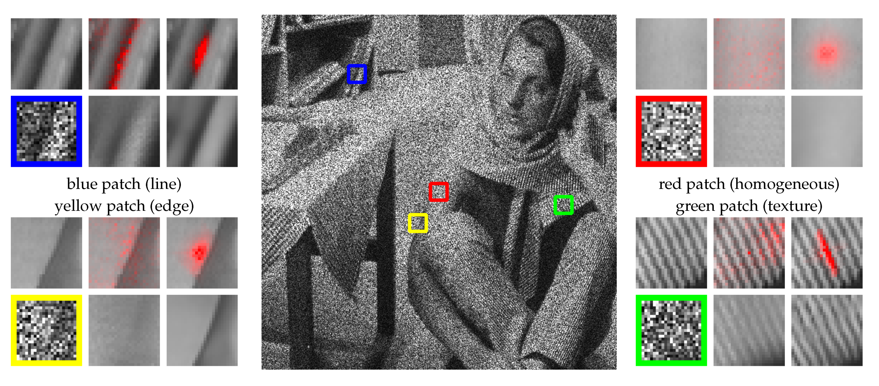
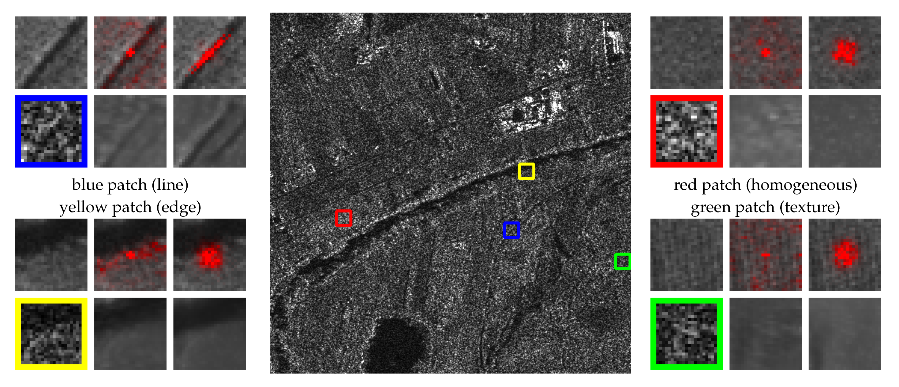
• suppress most of the speckle in homogeneous regions;
• preserve textures;
• preserve region boundaries and other linear structures;
• avoid altering natural or man-made permanent scatterers; and
• avoid introducing filtering artifacts.

Research on SAR image despeckling has been going on for several decades [6]. Early methods were based on spatial-domain filtering [7,8], with some forms of local adaptivity to deal with signal non-stationarity. In general, they ensure only a limited speckle reduction. Then, the diffusion of wavelet transform spawned a new generation of filters based on transform-domain coefficient shrinkage. For example, Xie et al. [9] used a Markov random field (MRF) prior to improve regularity in wavelet-domain shrinkage, while Solbo and Eltoft [10] performed homomorphic wavelet maximum a posteriori filtering. Despite a stronger speckle rejection, however, these methods ensured limited detail preservation and introduced disturbing artifacts. More recently, nonlocal methods gained large popularity due to their superior performance. The nonlocal approach was first proposed in the seminal paper of Buades et al. [11], together with the nonlocal means (NLM) algorithm for denoising images corrupted by additive white Gaussian noise (AWGN). Then, in [12], Dabov et al. proposed the highly effective block-matching 3D algorithm (BM3D), a de facto baseline in the field. These ideas and tools proved effective also for SAR despeckling, and several effective nonlocal despeckling filters were soon proposed, including PPB [13], SAR-BM3D [14], FANS [15], NL-SAR [16], and the NLM variants proposed in [17].

In the last few years, deep learning ensured a quantum leap in many image processing tasks in remote sensing, from land cover classification [18], to segmentation [19], pansharpening [20], and data fusion [21]. Therefore, there is a growing interest also for deep learning-based SAR image despeckling. Methods based on convolutional neural networks (CNN) [22,23] and generative adversarial networks (GAN) [24] have been proposed already back in 2017, and new methods keep appearing at a growing rate [25,26]. Nonetheless, improvements over the previous state of the art have been quite limited to date. This is probably due to the scarcity of high-quality training data, but also to a still insufficient comprehension of the despeckling problem and of the potential of deep learning methods towards its solution. Under this point of view, nonlocal methods are especially interesting as they shed some light on despeckling mechanisms. They rely on the idea of separating the filtering process in two key steps: (i) finding the best predictors of the target, not necessarily close to it; and (ii) performing the actual estimate based on them. The separate analysis of these two steps provides precious insight on method’s strengths and weaknesses.

In this work, we try to blend the nonlocal concept with CNN-based image processing, with the aim of exploiting their complementary strengths for SAR despeckling. Although some CNN-based nonlocal methods have been proposed for AWGN denoising, in the last few years (e.g., [27,28,29,30]), only very recently, researchers have begun to explore this promising approach for SAR despeckling [31,32]. In particular, here we follow our recent conference paper [31], and propose a simple CNN-powered nonlocal means filter, that is, plain pixel-wise nonlocal means in which the filter weights are computed by means of a dedicated convolutional network. By doing so, we pursue a two-fold goal. On the one hand, we look for sheer performance, aiming at improving objective and subjective quality indicators with respect to the current state of the art. On the other hand, we look for interpretable results, which shed light on the potential of this approach and on ways to achieve it. Therefore, we do not use deep learning to blindly separate signal from noise, but rather use a strongly constrained CNN-based architecture that provides interpretable results, in terms of relationships among target and predictor pixels. That is, we try to gain some new insights on SAR despeckling by studying the strategy followed by data-driven methods to address this problem.

Following the Introduction, in Section 2, we analyze the related work on deep learning-based despeckling. Then, in Section 3, we describe the proposed approach, with two implementations based on different CNN architectures. Section 4 presents experimental results on synthetic and real-world SAR data, while Section 5 discusses results. Finally, Section 6 draws conclusions and outlines future work.

2. Related Work

To the best of our knowledge, the first papers using deep learning for SAR image despeckling date back to 2017. The SAR-CNN proposed in [22] uses homomorphic processing to adapt the DnCNNN denoiser, proposed originally in [33] for AWGN data, to perform SAR despeckling. Training relies on 25-look SAR data taken as clean reference and a suitable SAR-oriented loss derived from the measure proposed in [13,34]. A significant performance improvement is observed with respect to state-of-the-art conventional methods, but the lack of truly clean (infinite-look) SAR data is pointed out as a major limiting factor to performance.

In addition, the Image Despeckling CNN (ID-CNN) proposed in [23] resorts to residual learning to estimate the noise component of the image. However, it works directly in the original domain, and the despeckled image is obtained by dividing the original image by the estimated noise, which seems to be an unreliable practice. To circumvent the problem of missing clean data, training is performed on simulated SAR images, obtained by injecting synthetic speckle on optical (e.g., GoogleEarth) images. A combination of Euclidean and Total Variation (TV) losses is used. This approach to training, call it synthetic, is followed by the majority of subsequent papers. Although it allows for virtually unlimited training data, they do not possess the statistical properties of real-world SAR images. The underlying clean signal differs from a true SAR signal (just think of the double reflection lines in urban areas) while the hypothesis of uncorrelated speckle holds only in special circumstances.

In [24], the same authors of [23] proposed a despeckling method based on Generative adversarial networks (GAN). During training, the discriminator distinguishes clean from despeckled images and teaches the generator how to extract high-quality clean images from the original SAR data. To this end, the Euclidean loss is complemented by a perceptual loss (computed on a pretrained VGG16 model [35]) and an adversarial loss. Again, synthetic training is used, casting doubt on the merits of an interesting approach. We also point out that the trained model is not published online, making it virtually impossible to replicate the experiments, given the hardship of GAN training.

In addition, inspired by Wang et al. [24] is SAR-DRN [36] based on a dilated residual network (DRN). Dilated convolutions allow one to keep the lightweight structure and small filter size of ID-CNN but enlarge the receptive field. In addition, skip connections help reduce the vanishing gradient problem. Along the same line, Gui et al. [37] used dilated convolution and residual learning with a densely connected network. In addition, Li et al. [38] relied on dilated convolution and residual training, the main innovation being the use of a convolutional block attention module to enhance representation power and performance. All these methods use synthetic training on the UC-Merced [39] dataset. Dense connections are used also in [40] to face the vanishing gradient problem, but, to further reduce computation, a limited block-wise connectivity is considered. Moreover, to help the network preserve image details, a preliminary single-level wavelet transform is computed, and the stacked subbands are fed to the net, using a loss function based on wavelet features. Again, synthetic training based on UC-Merced images is used.

In [41], the U-Net architecture, originally proposed for segmentation, is adapted to despeckling needs. The loss includes an additional total variation term to better filter smooth areas. After synthetic training on aerial images, the net is fine-tuned on more realistic simulated data, obtained by injecting speckle on multitemporal filtered SAR images. To avoid overfitting, speckle data are generated on the fly. A very simple denoiser is proposed in [42] with the goal to show the value of an additional loss term accounting for the Kullback–Leibler divergence between original and despeckled data, so as to ensure fidelity of first-order statistics. However, a very limited experimental validation is carried out.

Training on SAR data is completely bypassed in [43]. Following the MuLoG approach [44], the idea is to exploit denoising architectures designed for additive white Gaussian noise and pre-trained on abundant AWGN data. Suitable adaptation is applied to deal with Fisher–Tippet distributed log-transformed SAR data, which, for low number of looks, differ significantly from Gaussian data. Pan et al. [45] followed the same approach but replaced the DnCNN denoiser with the faster FFDNet denoiser [46], which uses combined downsampling-upsampling steps to improve efficiency. Then, in [25], homomorphic filtering is performed based on multiple instances of the same CNN [47] trained on Gaussian noise at various levels of intensity. The output images are then combined by means of guided filtering driven by an edge map.

A few very recent papers use noise2noise (N2N) training to circumvent the lack of truly clean SAR data. In [48], it is observed that a CNN denoiser can be trained effectively also in the absence of a clean ground truth provided multiple images with the same signal component and independent noise realizations are available. Therefore, clean targets can be replaced by noisy targets. The noise level of the noisy reference is immaterial (hence, blind despeckling is possible) and is only required that mean value is preserved. In [49], N2N training is used for a slightly modified version of U-Net. Later on, in [50], N2N training is applied to a dense dilated-convolution network without batch normalization. In both cases, however, the authors kept training on images with simulated speckle, hence the true potential of N2N training is never really exploited. A similar flaw affects the method in [51], where samples for N2N training are generated by means of a GAN architecture and a nested U-Net model is used for the final despeckling. In [52], a blind speckle decorrelator is used to pre-process test images and improve their fir to synthetic images used for N2N training.

To the best of our knowledge, the interplay between nonlocal methods and deep learning for SAR despeckling has been first explored in two very recent papers. In [32], the approach of Cruz et al. [29] is followed, in which nonlocal processing is used to refine the output of CNN-based filters. Instead, in [31], we proposed to use nonlocal means filtering with weights computed patch-by-patch by means of a dedicated CNN, so as to compare the weights provided by the network with those output by conventional nonlocal methods.

We conclude this short, and certainly non-exhaustive, review with some general remarks. First, it clearly appears that the use of deep learning for SAR despeckling is raising great interest, and new methods are being proposed by the day. Most of these proposals, however, focus on new architectures, neglecting what is the most critical point, in our view, i.e., the lack of reliable reference data. Synthetic training cannot really make up for this lack, and ad hoc datasets, such as in many other fields, are needed more than new architectures. A further observation is that many papers do not provide code and data to allow for reproducible research, also due to the restrictive policies on data widespread in the remote sensing field. Finally, we note an insufficient attention to previous methods and results. For example, for the well-known SAR-BM3D method, two papers report a ENL indicator below 5 and above 500,000, respectively, fluctuations that can be hardly attributed to differences in the original images.

3. Proposed Method

In this section, we motivate and describe the adopted nonlocal CNN filtering framework, and then propose two implementations of its core CNN, the first one based only on local convolutional layers, and the second one including also a recently proposed nonlocal layer.

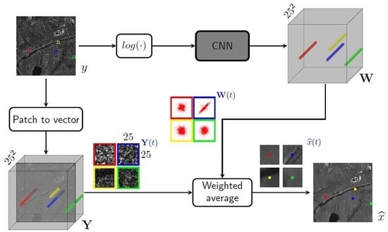
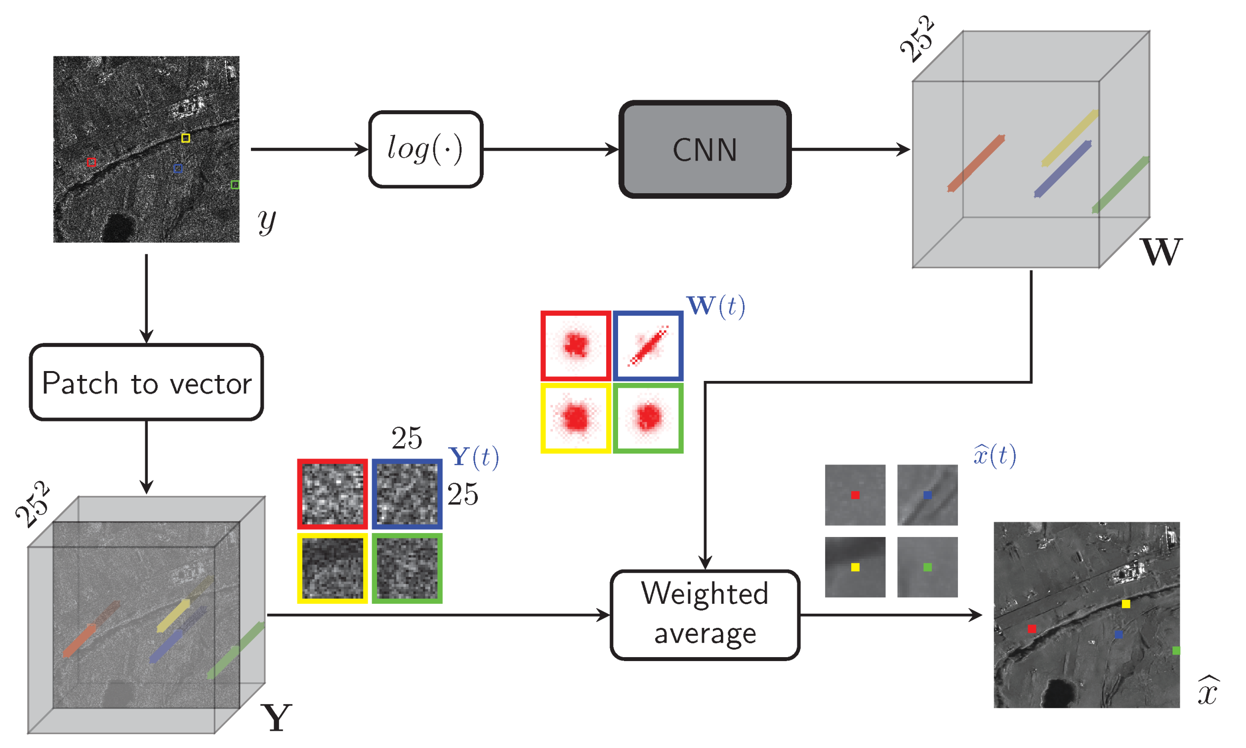
3.1. CNN-Powered Nonlocal Means

In [22], we already proposed a CNN-based despeckling filter, called SAR-CNN, based on residual training in the log-domain, obtaining a state-of-the-art performance. A weak point of that proposal, as well as of all deep learning-based methods, is the difficult interpretation of the results. The filter acts basically as a black box, and we can only observe the output produced in correspondence of a given input. A careful analysis may point out strengths and weaknesses of the method but not their origin and possible solution. Indeed, the problem of interpreting and controlling the network behavior is receiving much attention in the deep learning literature (e.g., [53,54]), but remains open today.

Based on such considerations, this work aims not only at improving performance with respect to the state of the art, but also at providing more interpretable results that can guide us towards future developments. Given the outstanding performance of nonlocal SAR despeckling methods, we propose an architecture which embodies nonlocal processing. However, we also make it interpretable, as far as possible, so as to gain insight into the overall potential of nonlocal processing in the context of CNN-based SAR image despeckling. With this goal in mind, we decided to consider the strongly constrained framework depicted in the block diagram of Figure 1, which implements plain pixel-wise nonlocal means (NLM) [11].

In NLM, each filtered pixel is obtained through the weighted sum of noisy pixels taken in a relatively large neighborhood, that is

$$\widehat{x}\left(t\right)=\sum _{s\in \mathsf{\Omega }\left(t\right)}w(s,t)y\left(s\right)$$

(1)

where $\widehat{x}\left(t\right)$ is the estimate of $x\left(t\right)$, the clean image at site t, $y\left(s\right)$ is a sample of the noisy image at site s, $\mathsf{\Omega }\left(t\right)$ is a neighborhood centered on t, and $w(s,t)$ is the weight of $y\left(s\right)$ in the estimate of $x\left(t\right)$. Crucial for the success of nonlocal means is the selection of suitable weights, such to exploit the dependencies among the target pixel and its noisy estimators. In [11], weights are made to depend on a measure of dis-similarity $d\left[x\right(s),x(t\left)\right]$ between estimator and target,

$$w(s,t)=C{e}^{-\lambda d\left[x\right(s),x(t\left)\right]}$$

(2)

with $\lambda$ a bandwidth parameter, governing filtering smoothness, and C a normalizing constant. Lacking any prior knowledge, besides the observed noisy data, this measure relies on patch-based contextual information, that is

$$d[x\left(s\right),x\left(t\right)]={\parallel \mathbf{y}\left(s\right)-\mathbf{y}\left(t\right)\parallel }^2$$

(3)

where $\mathbf{y}\left(t\right)$ and $\mathbf{y}\left(s\right)$ are two small patches centered on t and s, respectively. By using patches, rather than individual pixels, one takes into account the context and reduces the impact of noise on dissimilarity estimation. The choice of the Euclidean distance can be shown to be optimal in the AWGN case, while other distances are more suited to different noise distributions.

In this work, we keep using the pixel-wise NLM of Equation (1), but rely on a CNN to select the most appropriate weights for each target pixel. Given a large number of examples, we expect the CNN to learn how to best exploit spatial dependencies. It should be clear that pixel-wise NLM is far from the state of the art; much improved versions have been proposed in time, and filters based on the blending of multiple approaches, such as BM3D, are definitely more effective. However, besides the main goal of improving results, we aim at gaining insight into the CNN “reasoning”, and this is relatively easy based on the analysis of the NLM weights.

Going back to Figure 1, the clean signal at site t is estimated through NLM, based on the patch of noisy data extracted around it, $\mathbf{Y}\left(t\right)=\left\{y\right(s),s\in \mathsf{\Omega }(t\left)\right\}$. To fix the ideas, let t be the central pixel of the 25 × 25 patch highlighted with a blue frame in the input image (upper-left). $\widehat{x}\left(t\right)$ is simply given by the weighted average of $\mathbf{Y}\left(t\right)$ using weights $\mathbf{W}\left(t\right)$ computed by the CNN. On the upper path of the scheme, the whole input y is first log-transformed, and then fed to the CNN, which outputs the weights $\mathbf{W}\left(t\right)=\left\{w\right(s,t),s\in \mathsf{\Omega }(t\left)\right\}$ corresponding to each location t in form of ${25}^2$-vectors. Irrespective of the specific CNN architecture, its last layer is always a ${25}^2$-way softmax, so as to ensure non-negative weights with unitary sum over each patch-vector. Note that the log is only introduced to avoid the instabilities caused by the multiplicative nature of the speckle, and does not imply homomorphic processing. In fact, the SAR data are filtered in their original format, that is, the NLM block implements exactly the formula of Equation (1).

The key processing block is the CNN, responsible for selecting the best weights for each individual target. In the following subsection, we describe two alternative architectures, a more conventional one, already described in our preliminary conference paper [31], and a more innovative solution, proposed here for the first time, including new nonlocal layers. In Figure 2, the training scheme used for the first architecture is illustrated which, with straightforward modifications, can be adapted also to the second architecture. The lower part of the scheme coincides with the forward processing of Figure 1. In principle, a single noisy training patch $\mathbf{Y}\left(t\right)$ is processed to generate the weights, $\mathbf{W}\left(t\right)$, and hence the estimate, $\widehat{x}\left(t\right)$, of the central target pixel. This latter is then compared with the clean reference $x\left(t\right)$, to compute a loss which is back-propagated to update the CNN weights. In real operations, however, the training images are properly cropped to create minibatches, with multiple target pixels estimated at once, to allow an efficient implementation of the training on the available hardware. This process is also described synthetically in Figure 2.

As loss function we use the SAR-domain distance analyzed in [34]

$$\mathcal{L}(\widehat{x},x)=d_{\mathrm{SAR}}(\widehat{x},x)=log\left[(\widehat{x}+x)/\sqrt{\widehat{x}x}\right]$$

(4)

where image samples are in intensity format.

3.2. Estimating Weights with a Conventional CNN

We now consider a first implementation of the proposed framework based on a fully convolutional neural network. Layers and hyperparameters are summarized in

Table 1. Layers and parameters of the local core CNN.

Layer	Type	Spatial Support	Out. Features	Nonlin.	Batchnorm
1	conv	5 × 5	13${}^2$	leaky ReLU	n
2	conv	3 × 3	15${}^2$	leaky ReLU	y
3	conv	3 × 3	17${}^2$	leaky ReLU	y
⋮	⋮	⋮	⋮	⋮	⋮
11	conv	3 × 3	33${}^2$	leaky ReLU	y
12	conv	1 × 1	25${}^2$	none	n
13	softmax	25 × 25	25${}^2$	softmax	n

. There are 12 convolutional layers, with leaky ReLU nonlinearity and batch normalization (except for the first and last layer). All filters have 3 × 3 spatial support, to limit the number of parameters, except 5 × 5 in the first layer, while the number of features grows with the overall field of view, which reaches 25 × 25 in the last layers. In the 12th layer, the 1089 features are compressed to 625 to match the size of the filtering window, and then the softmax layer ensures meaningful weights.

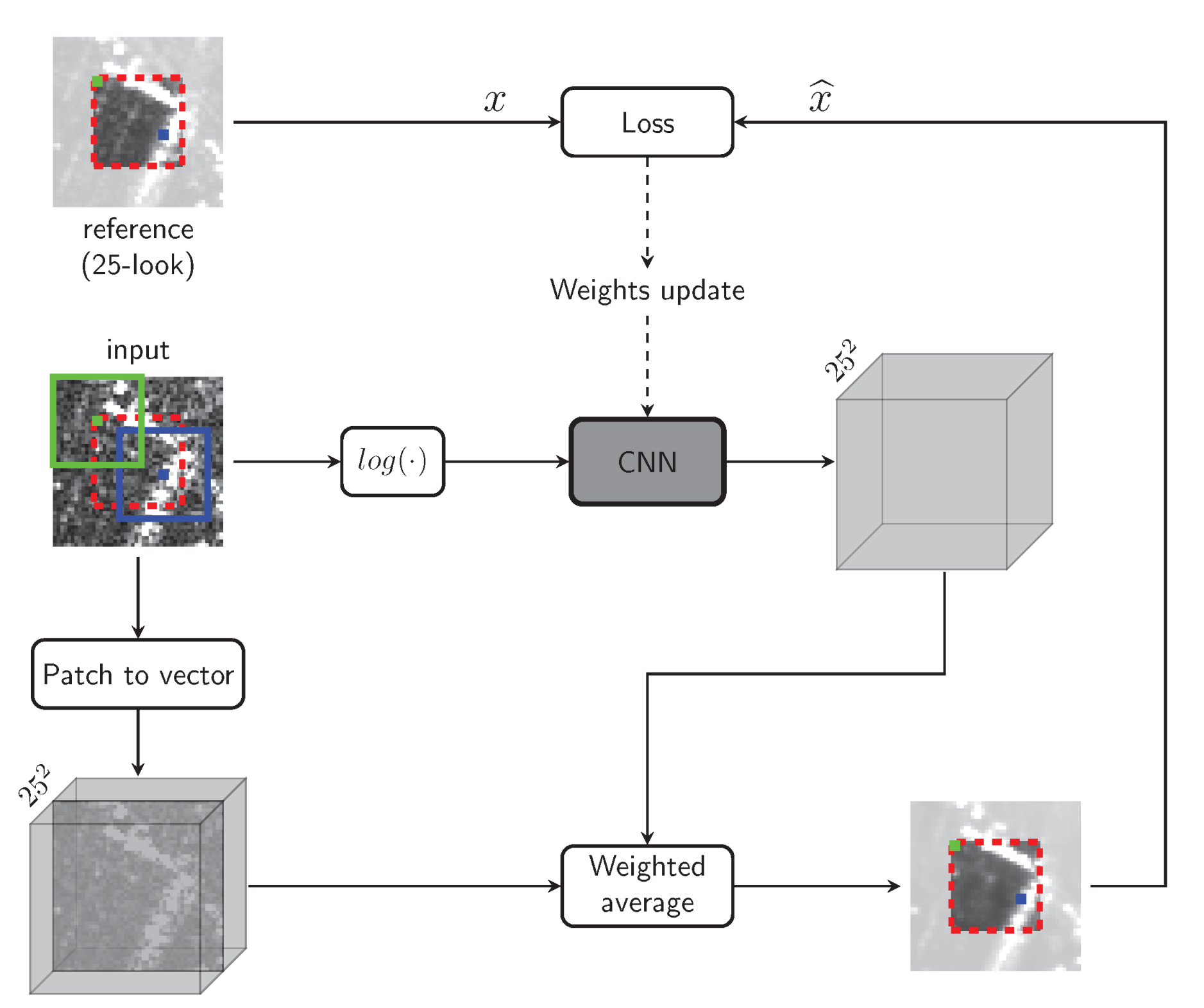
3.3. Estimating Weights with a “Nonlocal” CNN

With our second implementation, we try to encourage a stronger use of nonlocal information. Layers and hyperparameters of this new CNN are summarized in

Table 2. Layers and parameters of the nonlocal core CNN.

Layer	Type	Spatial Support	Out. Features	Nonlin.	Batchnorm
1÷5	conv	3 × 3	64	ReLU	y
6	conv + skip	3 × 3	8	ReLU	n
7	${\mathrm{N}}^3$	80 × 80	64	none	n
8÷12	conv	3 × 3	64	ReLU	y
13	conv + skip	3 × 3	8	ReLU	n
14	${\mathrm{N}}^3$	80 × 80	64	none	n
15÷19	conv	3 × 3	64	ReLU	y
20	conv	3 × 3	25${}^2$	softmax	n

. The main innovations with respect to the previous solution are the use of the ${\mathrm{N}}^3$ nonlocal layer and a quite larger overall field of view.

The ${\mathrm{N}}^3$ layer has been proposed recently [30] to enable nonlocal processing in any general-purpose convolutional network. To obtain such a result, the new layer must embody the principles of nonlocal processing in fully differentiable functions, so as to allow training by backpropagation. This is achieved by engineering a differentiable and continuous version of the K-nearest neighbors (K-NN) rule. Indeed, using nearest neighbors to pursue the task of interest is the quintessential nonlocal process. However, the K-NN selection rule is a non-differentiable function of the input features, and including it in a CNN would not allow backpropagation. Consider as an example the case $K=1$. Let q be the query (target feature) and $\mathcal{F}=\{f_1,\dots ,f_N\}$, a dataset of N features, with $q,f\in R^D$. The function ${\mathrm{NN}}_1:(q,\mathcal{F})\to {\{0,1\}}^N$ outputs a one-hot coded weight vector, ${\mathbf{w}}_1$ with components

$$w_1\left(i\right)=\left\{\begin{array}{cc}1\hfill & \mathrm{for}i=arg\underset{j}{max}[-d_j]\hfill \\ 0\hfill & \mathrm{otherwise}\hfill \end{array}\right.$$

(5)

where $d(·,·)$ is a suitable distance measure in $R^D$, for example the Euclidean distance, and $d_j=d(q,f_j)$. Now, if one of the features, say $f_k$, moves closer to q and becomes the new nearest neighbor, the two weights $w_1\left(i\right)$ and $w_1\left(k\right)$ switch instantaneously from 1 to 0 and vice versa.

A differentiable version of this function, however, is readily obtained by replacing the hard-max with the softmax function, that is

$${\tilde{w}}_1\left(i\right)=\frac{e^{-d_i/T}}{{\sum }_j{e}^{-d_j/T}}$$

(6)

where T is a temperature parameter, such that ${\tilde{\mathbf{w}}}_1\to {\mathbf{w}}_1$ as T approaches 0. Both for the hard and soft versions, the kth weight vector, associated with the kth NN, is obtained by using Equations (3) and (4), respectively, after setting to infinity the distances of the first $k-1$ NNs.

Besides being differentiable, the soft selection rule allows one to define the “continuous” nearest neighbors (cNN) of q,

$${\tilde{f}}^{\left(k\right)}=\sum _i{\tilde{w}}_k\left(i\right)f_i,k=1,\dots ,K$$

(7)

Again, as T approaches 0, these quantities converge to the conventional NNs ${\tilde{f}}^{\left(k\right)}\to f^{\left(k\right)}$. However, for $T\gg 0$, they amount to an average over of a large number of neighbors of the query. It is worth underlining that such smooth averages are largely used in nonlocal filtering to process homogeneous regions of the image.

We can now briefly discuss the architecture summarized in Table 2. The first six layers are borrowed from the AWGN denoiser proposed in [33], including the final skip connection, except for the last layer, which outputs only eight feature maps. Then, for each input feature vector, the subsequent ${\mathrm{N}}^3$ layer computes a local temperature and, based on this, the set of its seven cNNs. These are not combined in any way, but provided in output together with the input feature itself, relying on the net to learn the best way to use all this information. Note that the ${\mathrm{N}}^3$ layer has a quite large field of view, exploring (with stride 5) neighbors in a 80 × 80-pixel window. The six convolutional and the ${\mathrm{N}}^3$ layers are then repeated, and finally another group of six convolutional layers, followed by a softmax nonlinearity, provide the desired weights.

4. Experimental Validation

To assess the proposed approach, we carried out experiments on both simulated and real SAR images. Optical images with injected single-look speckle allowed us to compute objective performance indicators, the peak signal-to-noise ratio (PSNR), and the structural similarity (SSIM), which enabled a simple comparison, in ideal conditions, with the state of the art. However, a solid performance validation could only be based on the analysis of real-world SAR images. In the absence of a clean reference, we used visual inspection of despeckled and ratio images to assess the filters’ properties, especially for what concerns preservation of image details. Instead, speckle suppression ability was measured objectively through the equivalent number of looks (ENL) computed on homogeneous regions of the image and by means of the no-reference image quality index $\mathcal{M}$ proposed in [55,56].

To study the improvement with respect to the state of the art, we considered a number of reference methods, chosen both for their performance and their diffusion in the community. The enhanced-Lee [57] and Kuan [8] local filters operate in the spatial domain with adaptive windows (we used size 5 × 5 pixel) that follow the dominant signal structures. Turning to nonlocal filters, besides plain NLM [11], we considered its SAR-oriented iterative version, PPB [13], and the more advanced NL-SAR [16], together with nonlocal transform-domain shrinkage methods, SAR-BM3D [14] and FANS [15]. Finally, we compared results with two deep learning-based methods, SAR-CNN [22] and ID-CNN [23]. In all cases, the main parameters, e.g., search-area and window size, were set as suggested in the original papers, and the SAR-domain distance proposed in [13] was used. As for the proposed method, the two core CNNs were trained with the ADAM gradient-based optimization method with 32-patch minibatches, and patch-sizes of 48 × 48 and 104 × 104-pixel, respectively. Synthetic training data were obtained by injecting single-look simulated speckle on 400 different optical images. Real SAR data were acquired by the COSMO-SkyMed satellites. In this latter case, lacking true speckle-free data, we resorted to temporally multilooked images (25 dates) as reference, excluding patches where temporal changes occurred. The two datasets comprise a total of 8000 and 12,800 minibatches, respectively. Training proceeded for 50 epochs, with an initial learning rate of ${10}^{-3}$, divided by ten after every 20 epochs. All code was in Tensorflow, running on an Intel Xeon CPU at 2.10 GHz and an Nvidia P100 GPU. The trained models will be made available online upon publication of the present paper.

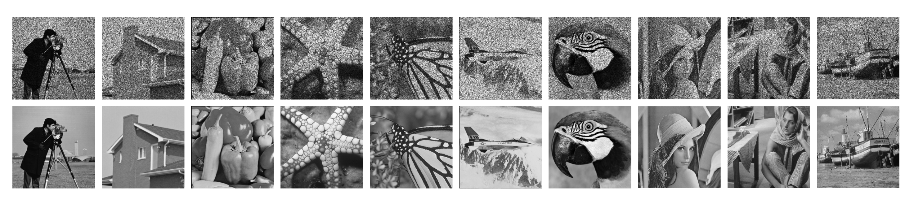
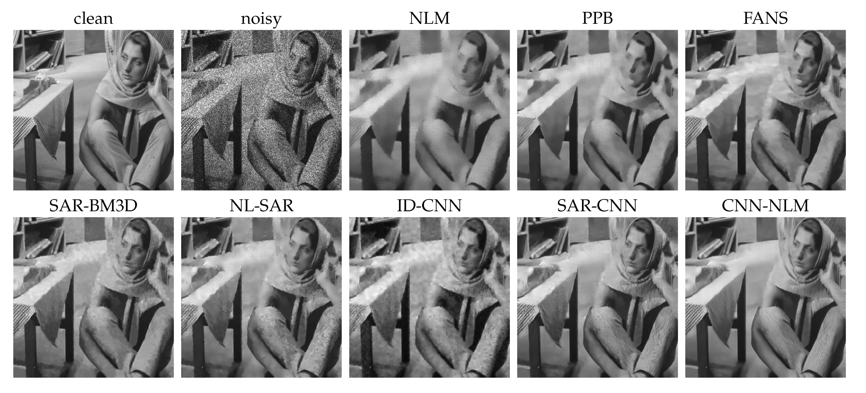
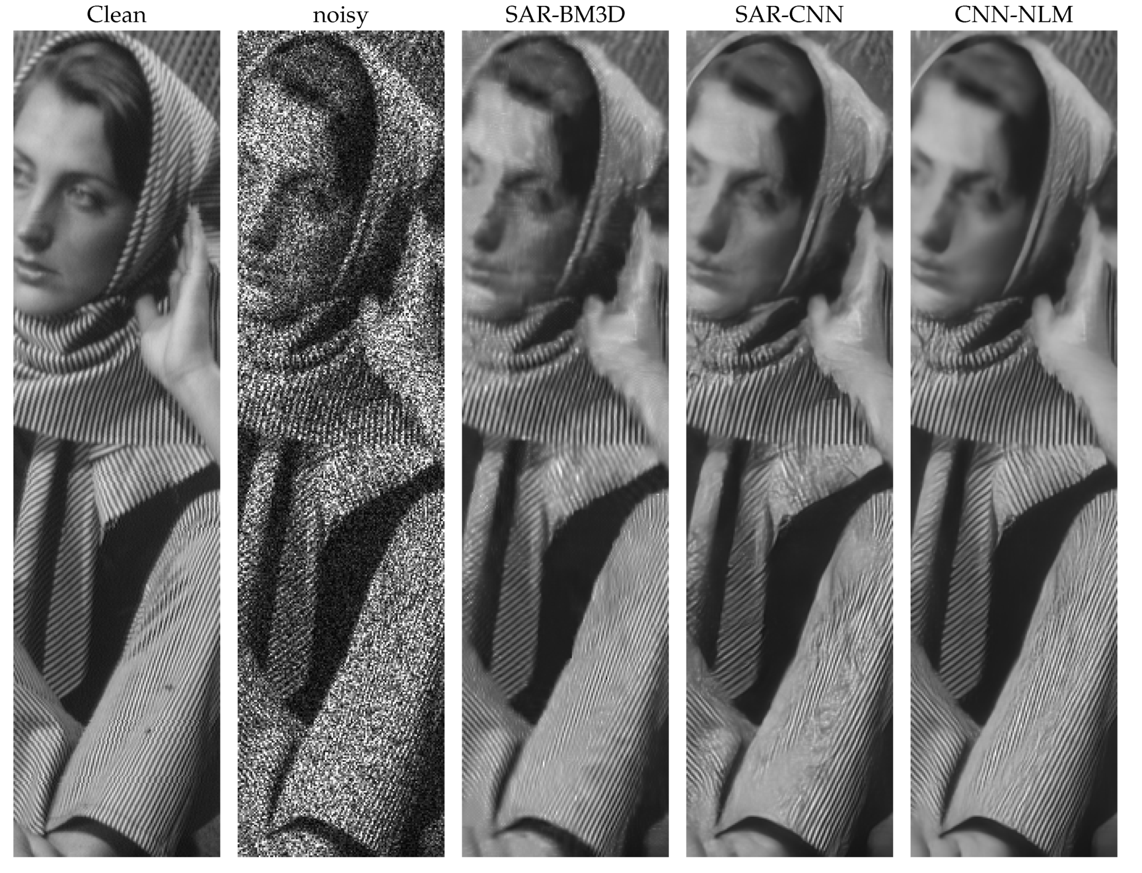
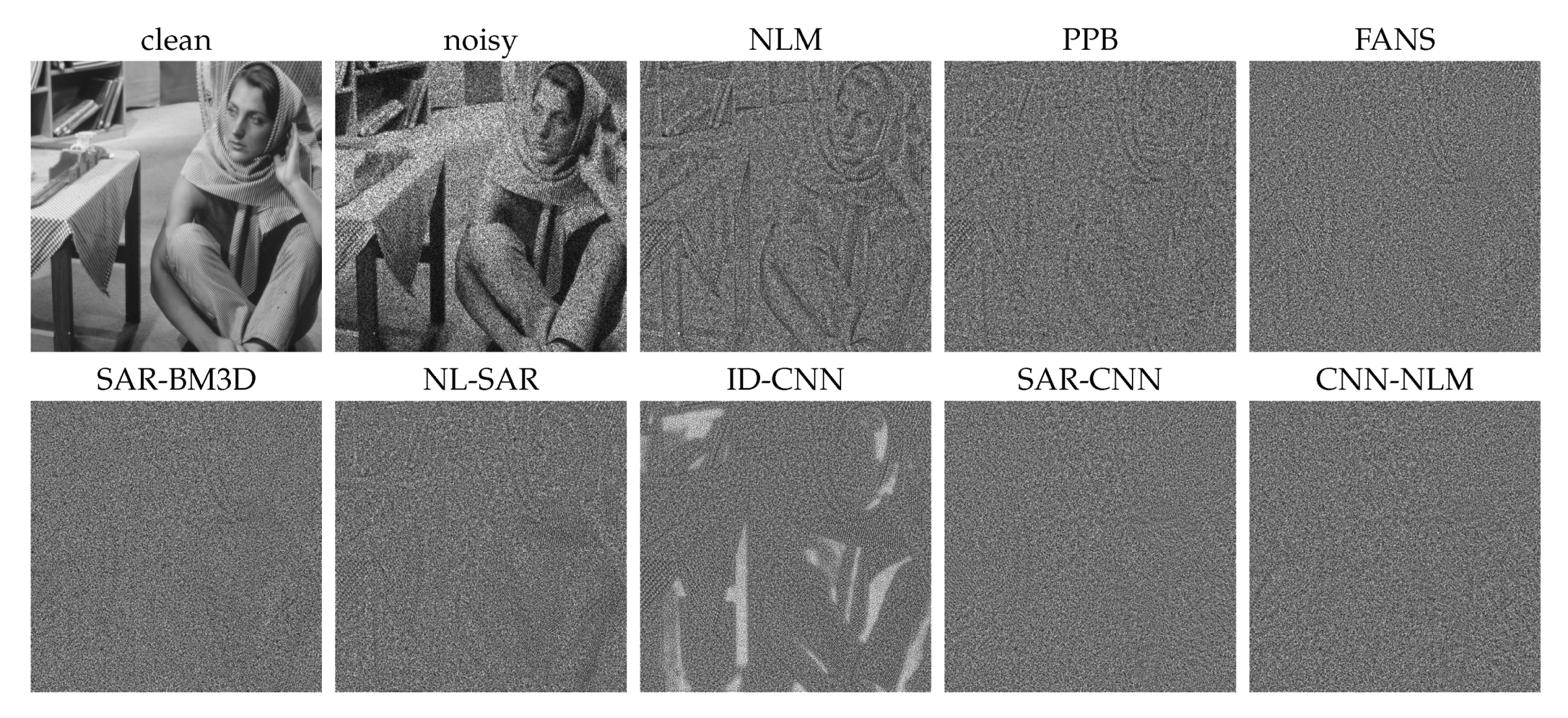
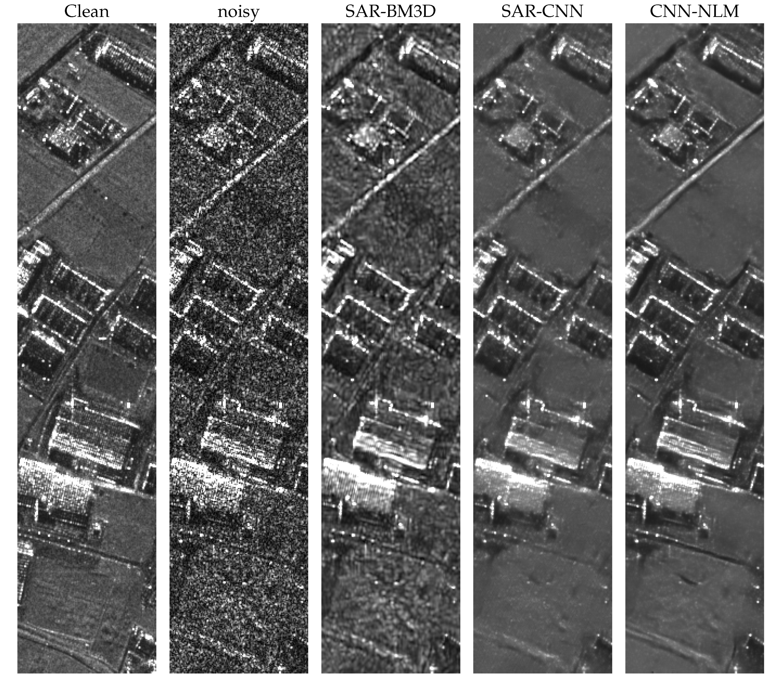
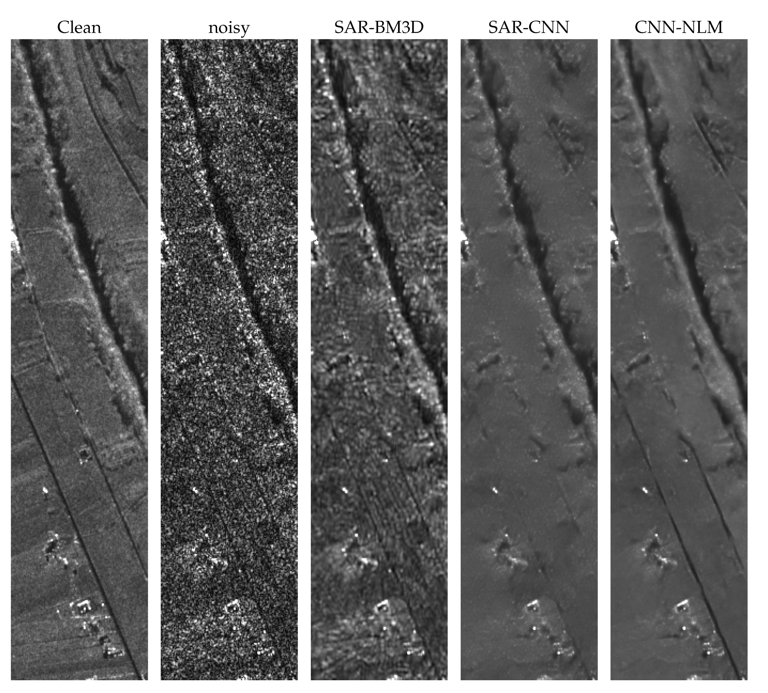
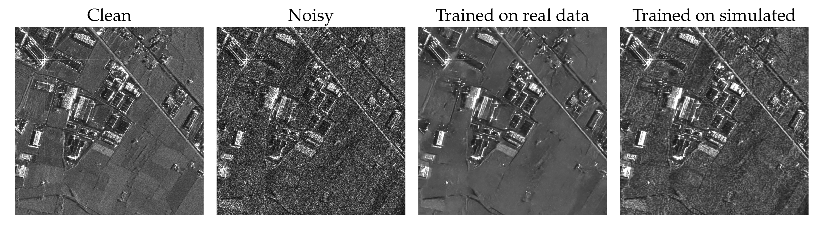
4.1. Experiments on Simulated Images

We generated simulated SAR images through the pixel-wise product of clean optical images with a field of Gamma-distributed independent random variables. In all our experiments, we considered only single-look images, since this is the most challenging case, due to the high intensity of speckle, and also the most interesting for applications, since there is no loss of resolution due to spatial multilooking.

In Figure 3, we show the clean and noisy images used in these experiments. Although in the despeckling literature it is customary to use optical remote sensing images for simulation purposes, we chose to consider general-purpose images to better remark that this approach does not generate faithful approximations of real-world SAR images in any case, and all results must be taken with due care. With these warnings, in

Table 3. Numerical results on simulated single-look images.

Method	PSNR	SSIM	TIME (s)
noisy	11.69	0.183	0.000
enhanced-Lee	20.95	0.474	0.012
Kuan	21.94	0.541	0.017
NLM	22.75	0.599	15.355
PPB	23.43	0.639	32.637
NL-SAR	24.01	0.678	5.944
SAR-BM3D	24.98	0.728	48.085
FANS	24.89	0.736	4.415
ID-CNN	24.22	0.687	0.014
SAR-CNN	25.95	0.762	0.029
CNN-NLM (w/o ${\mathrm{N}}^3$ layers)	25.96	0.758	0.036
CNN-NLM (with ${\mathrm{N}}^3$ layers)	26.45	0.786	0.360

, we show numerical results obtained on such images. Synthetic results were computed as the average over the 10 test images and, for each image, as the average over 10 realizations of the speckle field. Conventional methods are grouped on the upper part of the table, while methods based on deep learning are in the lower part.

Looking at the PSNR indicator, deep learning-based methods appear to have the potential to provide a clear performance gain over conventional ones. Indeed, while ID-CNN is aligned with advanced nonlocal methods, SAR-CNN improves by about 1 dB over the best of them (SAR-BM3D). As for the proposed method, there is no further improvement with respect to SAR-CNN when the NLM weights are estimated with a fully-convolutional CNN. However, about 0.5 dB is gained when the CNN with nonlocal layers is used. Since this is a consistent behavior, in the following experiments we considered only this latter version of the proposed method. Turning to SSIM, quite a similar behavior was observed. The proposed method (with nonlocal layers) provides the best performance with an appreciable improvement over SAR-CNN, and a more significant gain with respect to all conventional methods. In the last column, we report the average processing time. With nonlocal methods, this was an issue. As an example, SAR-BM3D requires about 50 s of CPU, mostly for nearest neighbor search. This is orders of magnitude more than simpler local filters, such as Lee and Kuan, which in fact keep being popular among practitioners also for this reason. For deep learning methods, processing time becomes fully manageable again, provided a GPU is used. Of course, training the models may take very long, but this is carried out off-line.

To gain some insight into the quality of filtered images, Figure 4 shows the output of the best performing methods for the Barbara image. To allow for an overall view of results, and also to limit space, we display these images in a compact format. A suitable zooming is therefore recommended for accurate visual inspection of details. Considering the very noisy input, it seems safe to say that the proposed method provides filtered images of impressive quality. The speckle is effectively suppressed without significantly impairing the image resolution. Moreover, most details are well preserved, even thin lines and complex textures, and no major artifacts are introduced. Even the best conventional nonlocal methods, instead, fail under one or the other of these aspects. For example, SAR-BM3D preserves resolution and details, but ensures only a limited speckle suppression, while NL-SAR removes most speckle but at the price of a significant loss of resolution. As for plain NLM, based on the same filtering engine as the proposed method, it causes a strong loss of resolution, only partially solved with PPB. The most interesting comparison, however, is with SAR-CNN. To better appreciate the improvements, Figure 5 shows a much enlarged strip of Barbara, chosen for the abundance of patterns. Indeed, on such regular patterns, the improvement granted by the new method is striking, with lines that are barely distinguishable in the noisy input that are correctly reproduced in output most of the times. Moreover, the disturbing artifacts produced by both SAR-BM3D and SAR-CNN on Barbara’s face do not longer occur. Nonetheless, the loss of quality with respect to the clean image is still significant. Our sensitivity to the features of a human face allow us to fully appreciate the sharp loss of details that actually occurs. Whether a despeckling engine can ever avoid such losses, without the help of further information, is debatable.

To complete the analysis on simulated images, Figure 6 shows the ratio images for Barbara, that is, the ratios between the noisy input and the despeckled output. An ideal filter should remove only the injected speckle, therefore the ratio image should be a field of uncorrelated speckle samples. This seems to be actually the case for some filters, such as SAR-BM3D, SAR-CNN, and CNN-NLM, while, in some other cases, notably for NLM and PPB, there is a clear leakage of signal structures in the ratio image. ID-CNN, instead, seems to have a bias in very dark regions. The proposed method seems very satisfactory also under this point of view. This is also confirmed numerically by the no-reference quality index $\mathcal{M}$ [55,56], which compares the statistical distribution of the ratio image with that of the theoretical speckle. The analysis was carried out on a set of homogeneous areas of the image, automatically selected by the method. Results are reported in

Table 4. $\mathcal{M}$ quality indicator [55] on simulated test images.

Method	#1	#2	#3	#4	#5	#6	#7	#8	#9	#10	Average
enhanced-Lee	50.70	20.89	49.80	21.80	34.40	28.15	84.86	14.71	15.68	20.57	34.16
Kuan	89.14	20.04	39.24	16.26	52.95	31.32	107.86	12.10	11.27	20.51	40.07
NLM	21.85	17.26	15.99	12.78	27.59	31.52	44.40	12.19	7.57	16.87	20.80
PPB	10.10	13.57	11.29	11.45	15.06	13.93	24.23	7.00	7.51	8.22	12.24
NL-SAR	15.84	15.47	26.24	12.52	19.25	14.54	33.40	6.55	9.49	7.81	16.11
SAR-BM3D	15.92	12.55	10.37	15.25	15.67	13.33	42.46	6.15	7.62	8.12	14.74
FANS	10.41	9.41	9.04	8.87	12.86	7.41	19.91	2.96	6.46	5.21	9.25
ID-CNN	50.08	33.37	3.69	10.08	178.12	3.76	55.74	26.82	3.82	11.01	37.65
SAR-CNN	15.57	11.75	11.84	14.06	14.81	10.64	20.14	4.94	7.03	6.52	11.73
CNN-NLM	11.55	9.62	9.89	11.75	11.73	9.11	19.24	4.03	6.72	4.90	9.85

for each test image, with smaller values (zero in the ideal case) indicating better performance. The proposed method always exhibits one of the smallest values (best in boldface) and the second smallest on the average.

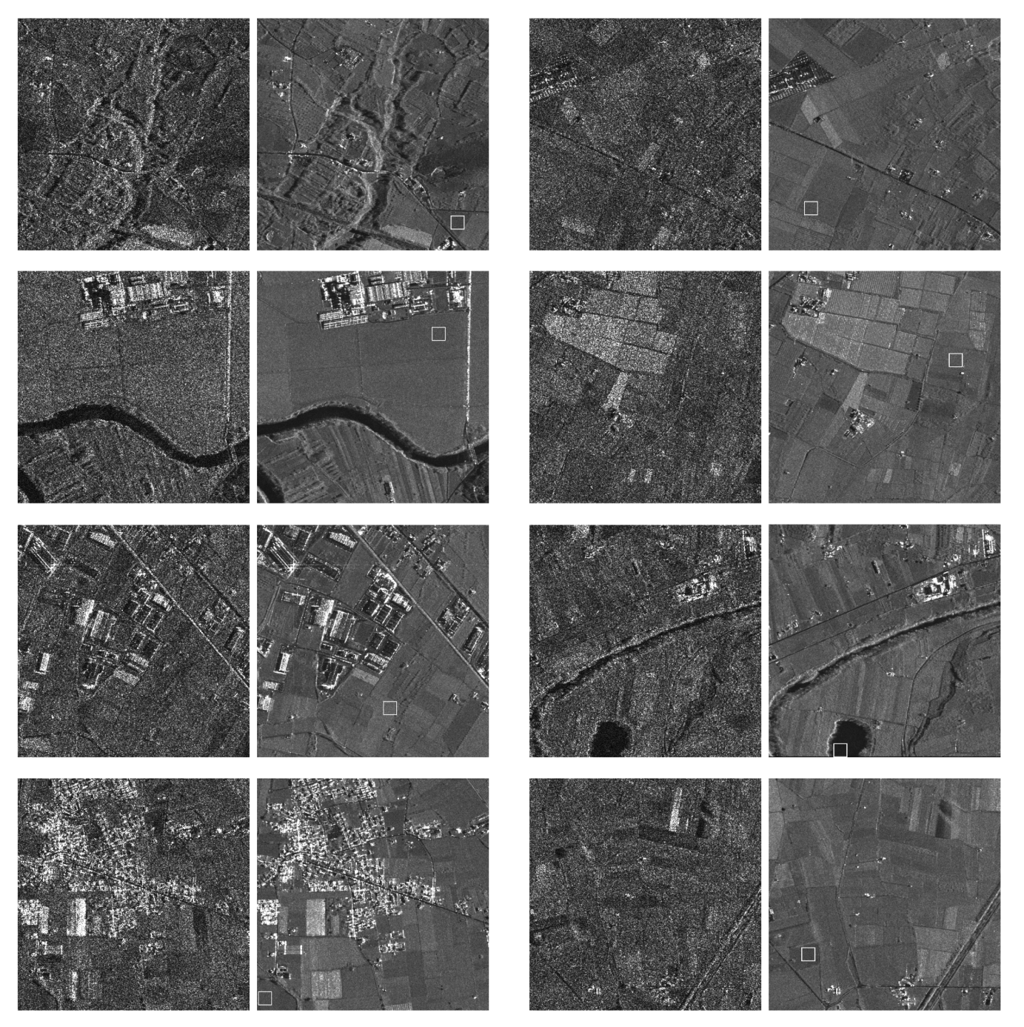
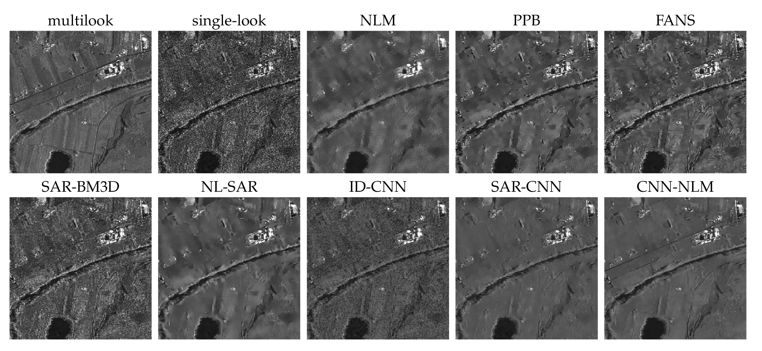
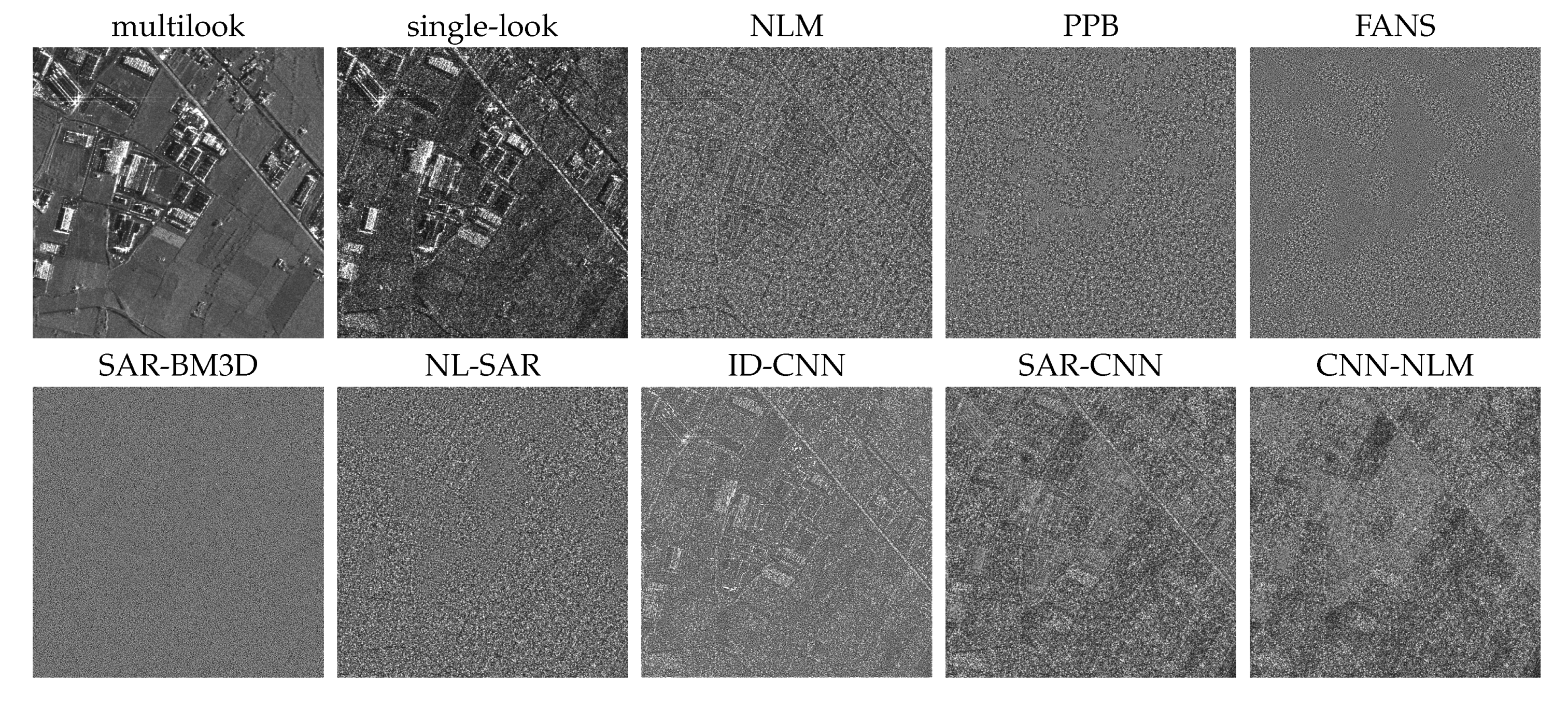
4.2. Experiments on Real-World SAR Images

To validate the proposed method on real-world SAR data, we relied on a stack of 25 co-registered single-look images acquired by the COSMO-SkyMed sensor over the city of Caserta (I), and spanning a temporal interval of about five years, from 26 July 2010 to 23 March 2015. The images cover an area of about 40 km × 40 km, with 3 m/pixel spatial resolution, for a size exceeding 16,000 × 16,000 pixels. Despeckling experiments were all carried on the first image of the stack. Temporal multilooking was used to obtain reference data for training. Of course, such reference is far from the ideal “clean” data, not only for the limited number of looks, which implies imperfect rejection of speckle, but also for the presence of temporal changes. The latter problem was addressed by discarding areas where a significant temporal change was detected. Eight 600 × 600-pixel clips were cropped from the first image and used for testing, sampling various types of land cover. Of course, these areas were excluded from the training set, but nearby areas of similar characteristics were included, so as to guarantee a good alignment between training and testing data. All test clips are shown in Figure 7 together with the corresponding multilook reference. Note that these multilooked images were not used in any way in validation (they even include regions in which temporal changes occurred) and are only shown to gain some insight into how the clean SAR signal might appear. The white boxes on the multilooked images indicate the regions used to compute the ENL.

Table 5. ENL on test images.

Method	#1	#2	#3	#4	#5	#6	#7	#8	Average
noisy	0.98	1.00	1.01	1.01	0.98	0.98	0.99	0.99	0.99
enhanced-Lee	7.69	8.43	6.72	8.63	8.12	7.99	9.14	7.07	7.97
Kuan	14.37	16.74	12.17	16.69	15.14	15.32	15.85	14.35	15.08
NLM	41.54	84.96	33.57	58.15	51.15	49.25	41.31	62.79	52.84
PPB	43.34	101.19	24.70	42.84	45.94	49.43	38.98	27.29	46.71
NL-SAR	59.95	97.17	150.31	131.86	97.72	43.73	102.26	134.14	102.14
SAR-BM3D	5.58	7.85	4.78	6.90	5.01	6.92	6.19	5.90	6.14
FANS	24.35	81.14	16.16	27.34	29.35	30.38	29.88	19.49	32.26
ID-CNN	5.76	9.52	8.10	8.99	6.37	2.82	8.40	6.77	7.09
SAR-CNN	24.97	237.09	177.40	317.63	64.92	117.69	175.53	73.54	148.60
CNN-NLM	316.84	464.88	235.08	271.52	94.18	171.39	346.70	100.19	250.10

reports, for each filter, the ENL measured on all test images and, on the rightmost column, their average. It appears that the proposed CNN-NLM provides always the largest (six images) or second largest (two images) ENL. This reflects in the largest average ENL (about 250) followed by CNN-SAR (150) and NL-SAR (100).

With real-world SAR images, however, even more than with simulated images, visual inspection is necessary for a solid assessment. Therefore, in the following figures, we show detailed visual results for two selected images. Again, for the sake of compactness, we display rather small images which require adequate zooming for analysis, except for two strips shown much enlarged and analyzed in depth later on. In Figure 8 and Figure 9, we show the output of selected filters for Images #5 and #6, respectively, together with the single-look input and the 25-look reference. Visual inspection confirms the good behavior of the proposed method. There is a very effective suppression of speckle, as predicted by the ENL numbers of Table 5, but also a faithful preservation of relevant details, such as man-made structures, field boundaries, and roads, which all keep their original high resolution. In addition, other methods preserve image resolution and details, such as SAR-BM3D, but with very limited speckle suppression. On the other hand, NL-SAR and SAR-CNN suppress speckle very well, but they also degrade resolution or lose entire structures. With the aim of better appreciating such differences, Figure 10 and Figure 11 focus on two narrow horizontal strips of Images #5 and #6 (rotated for better displaying) showing the output of SAR-BM3D, SAR-CNN and the proposed method next to the single-look input and the 25-look reference. As we observed before, SAR-BM3D seems to preserve all the information present in the input, without losing or even blurring informative details, but does not remove much speckle. SAR-CNN, instead, removes speckle very effectively but tends to lose or blur linear structures (roads and boundaries), which, instead, are very well preserved by the proposed method. This is arguably a consequence of nonlocal layers’ ability to take advantage of image self-similarities.

However, turning to the ratio images, shown in Figure 12 for SAR Image #5, we observed also an undesired behavior. The ratio images of all deep learning methods exhibit a clear leakage of signal, concerning not only linear structures but also the average intensity of some fields. Given the black-box nature of CNNs, we have only an indirect explanation for this phenomenon. However, the fact that it involves both our deep learning methods, and it happens only with SAR images and not with simulated data, may suggest that this problem has to do with the imperfect reference images used in training. In fact, a 25-look image is not the clean SAR signal, but only an approximation of it, based on temporal multilooking. Indeed, the fields characterized by a different average intensity than the rest of the image correspond to areas where the despeckled image approximates fairly well the reference (see again Figure 8) but not the original noisy image. Thus, the CNN behaves as instructed to do based on bad examples, probably due to seasonal changes that escaped the change detector. With these premises, the ratio image-based $\mathcal{M}$ index can only provide bad results, which is in fact the case, as shown in

Table 6. $\mathcal{M}$ quality indicator [55] on real SAR test samples.

Method	#1	#2	#3	#4	#5	#6	#7	#8	Average
enhanced-Lee	18.54	14.12	21.39	23.92	16.01	14.88	30.48	17.81	19.64
Kuan	15.18	9.09	31.21	14.78	17.14	14.43	63.89	13.60	22.41
NLM	11.80	9.74	16.54	9.78	9.75	8.59	19.80	10.19	12.02
PPB	10.44	12.44	14.36	11.93	7.89	8.74	27.75	10.10	12.96
NL-SAR	8.64	11.34	6.66	6.04	4.00	5.95	17.20	3.69	7.94
SAR-BM3D	28.13	27.27	26.52	30.14	30.26	27.88	33.17	29.28	29.08
FANS	7.60	12.33	15.12	10.46	9.04	10.09	25.63	8.68	12.37
ID-CNN	12.06	9.16	11.86	11.27	9.43	10.32	9.69	9.71	10.44
SAR-CNN	13.12	12.83	37.99	40.64	44.42	16.16	67.93	16.06	31.14
CNN-NLM	32.60	20.47	33.33	43.38	60.31	13.11	71.82	21.65	37.09

, where the proposed method trails all others. If our conjecture is right, however, these problems will be automatically solved when better reference data will be available, the first item in our agenda.

In alternative, one may be tempted to use the network trained on synthetic data, optical images with injected speckle, far from true SAR data but perfectly reliable and virtually unlimited. Figure 13 shows the output for SAR Image #5. Speckle suppression is much worse than with the network trained on our 25-look reference (output shown again for easier comparison) and some odd micropatterns appear in the despeckled image confirming that using real-world SAR data for training is the right way to go.

5. Discussion

We propose our CNN-NLM architecture with two goals: improving performance and providing some new insight into nonlocal filtering. Therefore, we now turn to study the weights generated by the proposed method and compare them with those of conventional NLM. Indeed, the only difference between the two methods is in the weights, generated by a CNN in the proposal, set on the basis of a similarity measure in NLM. Thus, we selected some relevant patches from Barbara and SAR Image #6, and analyzed the weights used to estimate their central pixel. The results are shown in Figure 14 and Figure 15, respectively. The selected patches are characterized by the presence of lines (blue), edges (yellow), and texture (green), or else are homogeneous (red). These structures are easily recognized in the clean/25-look reference patches, and much less in the original noisy ones. For each test patch, we built a subfigure showing, in the top row, the clean/multilook reference, and the weights selected by NLM and CNN-NLM superimposed to it, and, in the bottom row, the noisy input and the despeckled output provided by NLM and CNN-NLM.

Consider for example the blue patch from Barbara, and the associated subfigure in the top-left. Diagonal structures are clearly visible in the clean patch, especially a dark line in the center, the dark space between two books. Both the conventional and CNN-based weights follow this dark line to estimate the (dark) central pixel. In the first case, however, weights are dispersed over the whole patch, and gather information also from pixels farther away from the target, while the CNN weights are much more concentrated. The first choice is more adherent to the spirit of nonlocal filtering, as it tries to exploit relevant information all over the image. Nonetheless, results speak clearly in favor of the second choice. CNN-NLM provides in output quite a faithful copy of the clean signal, while the NLM output patch exhibits a clear loss of resolution and the dark line almost disappears. This can be explained by looking at how noisy the input patch is. Although sensible, in principle, the NLM choice of weights is quite risky, as it relies on a similarity measure that, in the presence of such noisy data, may select bad predictors.

This is even clearer in the second example, the yellow patch from Barbara, featuring a sharp edge. Due to the limited contrast between the dark and bright sides of the edge, and to the intense noise, NLM selects large weights on both sides, with the effect of largely smoothing the edge. On the contrary, all large CNN-NLM weights are on the right side of the edge, and allow for its faithful reproduction.

Of course, risky NLM weights are less of a problem in homogeneous areas (red patch) and they only give rise to some residual noise in the output patch, which is not necessarily wrong. Instead, in the presence of regular patterns (green patch), the dispersion of weights in a large area leads to blurred patterns in output, while the CNN weights, mostly concentrated on the central line, allow for the extraction of such hidden pattern.

In real-world SAR images, we observe the very same phenomena described before, only less pronounced, because of the absence of the sharp contrasts observed in optical images (we do not analyze strong scatterers or double reflection lines as they are always well reproduced by reasonably well-behaved filters). Again, lines (blue patch) are severely smoothed by NLM and tend to disappear because too many pixels are used for the estimate, and not all of them are reliable. Similar problems affect the edges (yellow patch) but are less pronounced. Homogeneous regions are correctly filtered in both cases, with the CNN weights ensuring only a stronger smoothing. Finally, we could find only some subtle regular patterns in our SAR image (green patch), so faint that the CNN could not find preferential directions, and both NLM and CNN-NLM largely smooth it out.

6. Conclusions

We propose a new method for SAR image despeckling, based on nonlocal filtering and deep learning (Supplementary Materials). The filter performs plain nonlocal means, but the filter weights are chosen through a properly trained CNN, featuring suitable nonlocal layers. The results are extremely promising, definitely competitive with the state of the art. A strong speckle rejection is observed, together with a faithful preservation of details. On the down side, we observed some signal leakages in the ratio images, which indicate imperfect filtering. Since this occurs only with real-world SAR images, we believe this is due to the low-quality reference images used for training. Besides performance, the analysis of CNN-generated weights sheds some light on the potential and limits of nonlocal filtering. Apparently, a careful use of nonlocality is recommended in the presence of very noisy data.

Despite the good performance of the proposed method, several issues call for further investigation. First, the signal leakage problem underlines the need for better training data and training modalities. In our opinion, the lack of reliable reference images is the primary factor limiting the performance of deep learning-based SAR despeckling. Then, we want to expand the analysis of NLM weights, to confirm our conjectures and explore more general cases. Finally, and most important, we aim at designing better despeckling methods. This could require the use of more elaborate filtering structures and the design and training of better deep learning architectures.

References

1. Zhang, H.; Lin, H.; Li, Y. Impacts of Feature Normalization on Optical and SAR Data Fusion for Land Use/Land Cover Classification. IEEE Geosci. Remote Sens. Lett. 2015, 12, 1061–1065. [Google Scholar] [CrossRef]
2. Baghdadi, N.; Hajj, M.; Zribi, M.; Fayad, I. Coupling SAR C-Band and Optical Data for Soil Moisture and Leaf Area Index Retrieval Over Irrigated Grasslands. IEEE J. Sel. Top. Appl. Earth Obs. Remote Sens. 2016, 9, 1229–1243. [Google Scholar] [CrossRef] [Green Version]
3. Scarpa, G.; Gargiulo, M.; Mazza, A.; Gaetano, R. A CNN-Based Fusion Method for Feature Extraction from Sentinel Data. Remote Sens. 2018, 10, 236. [Google Scholar] [CrossRef] [Green Version]
4. Vitale, S.; Cozzolino, D.; Scarpa, G.; Verdoliva, L.; Poggi, G. Guided Patchwise Nonlocal SAR Despeckling. IEEE Trans. Geosci. Remote Sens. 2019, 57, 6484–6498. [Google Scholar] [CrossRef] [Green Version]
5. Gragnaniello, D.; Poggi, G.; Scarpa, G.; Verdoliva, L. SAR despeckling by soft classification. IEEE J. Sel. Top. Appl. Earth Obs. Remote Sens. 2016, 9, 2118–2130. [Google Scholar] [CrossRef]
6. Argenti, F.; Lapini, A.; Bianchi, T.; Alparone, L. A tutorial on speckle reduction in synthetic aperture radar images. IEEE Geosci. Remote Sens. Mag. 2013, 1, 6–35. [Google Scholar] [CrossRef] [Green Version]
7. Lee, J. Speckle Analysis and Smoothing of Synthetic Aperture Radar Images. Comput. Graph. Image Process. 1981, 17, 27–32. [Google Scholar] [CrossRef]
8. Kuan, D.; Sawchuk, A.; Strand, T.; Chavel, P. Adaptive Noise Smoothing Filter for Images with Signal-Dependent Noise. IEEE Trans. Pattern Anal. Mach. Intell. 1985, 7, 165–177. [Google Scholar] [CrossRef]
9. Xie, H.; Pierce, L.; Ulaby, F. SAR speckle reduction using wavelet denoising and Markov random field modeling. IEEE Trans. Geosci. Remote Sens. 2002, 40, 2196–2212. [Google Scholar] [CrossRef] [Green Version]
10. Solbo, S.; Eltoft, T. Homomorphic wavelet-based statistical despeckling of SAR images. IEEE Trans. Geosci. Remote Sens. 2004, 42, 711–721. [Google Scholar] [CrossRef]
11. Buades, A.; Coll, B.; Morel, J.M. A review of image denoising algorithms, with a new one. Multiscale Model. Simul. 2005, 4, 490–530. [Google Scholar] [CrossRef]
12. Dabov, K.; A. Foi, A.; Katkovnik, V.; Egiazarian, K. Image denoising by sparse 3-D transform-domain collaborative filtering. IEEE Trans. Image Process. 2007, 16, 2080–2095. [Google Scholar] [CrossRef] [PubMed]
13. Deledalle, C.A.; Denis, L.; Tupin, F. Iterative weighted maximum likelihood denoising with probabilistic patch-based weights. IEEE Trans. Image Process. 2009, 18, 2661–2672. [Google Scholar] [CrossRef] [PubMed] [Green Version]
14. Parrilli, S.; Poderico, M.; Angelino, C.; Verdoliva, L. A nonlocal SAR image denoising algorithm based on LLMMSE wavelet shrinkage. IEEE Trans. Geosci. Remote Sens. 2012, 50, 606–616. [Google Scholar] [CrossRef]
15. Cozzolino, D.; Parrilli, S.; Scarpa, G.; Poggi, G.; Verdoliva, L. Fast adaptive nonlocal SAR despeckling. IEEE Geosci. Remote Sens. Lett. 2014, 11, 524–528. [Google Scholar] [CrossRef] [Green Version]
16. Deledalle, C.A.; Denis, L.; Tupin, F.; Reigber, A.; Jäger, M. NL-SAR: A unified nonlocal framework for resolution-preserving (Pol)(In)SAR denoising. IEEE Trans. Geosci. Remote Sens. 2015, 53, 2021–2038. [Google Scholar] [CrossRef] [Green Version]
17. Penna, P.A.; Mascarenhas, N.D. (Non-) homomorphic approaches to denoise intensity SAR images with non-local means and stochastic distances. Comput. Geosci. 2018, 111, 127–138. [Google Scholar] [CrossRef]
18. Castelluccio, M.; Poggi, G.; Sansone, C.; Verdoliva, L. Land use classification in remote sensing images by convolutional neural networks. arXiv 2015, arXiv:1508.00092. [Google Scholar]
19. Marmanis, D.; Wegner, J.; Galliani, S.; Schindler, K.; Datcu, M.; Stilla, U. Semantic segmentation of aerial images with an ensemble of CNNs. ISPRS Ann. Photogramm. Remote Sens. Spat. Inf. Sci. 2016, 3, 473–480. [Google Scholar] [CrossRef] [Green Version]
20. Masi, G.; Cozzolino, D.; Verdoliva, L.; Scarpa, G. Pansharpening by convolutional neural networks. Remote Sens. 2016, 8, 594. [Google Scholar] [CrossRef] [Green Version]
21. Yuan, Y.; Zheng, S.; Lu, X. Hyperspectral image superresolution by transfer learning. IEEE J. Sel. Top. Appl. Earth Obs. Remote Sens. 2017, 10, 1963–1974. [Google Scholar] [CrossRef]
22. Chierchia, G.; Cozzolino, D.; Poggi, G.; Verdoliva, L. SAR image despeckling through convolutional neural networks. In Proceedings of the IEEE International Geoscience and Remote Sensing Symposium (IGARSS), Fort Worth, TX, USA, 23–28 July 2017; pp. 5438–5441. [Google Scholar]
23. Wang, P.; Zhang, H.; Patel, V. SAR Image Despeckling Using a Convolutional Neural Network. IEEE Signal Process. Lett. 2017, 24, 1763–1767. [Google Scholar] [CrossRef] [Green Version]
24. Wang, P.; Zhang, H.; Patel, V. Generative adversarial network-based restoration of speckled SAR images. In Proceedings of the IEEE 7th International Workshop on Computational Advances in Multi-Sensor Adaptive Processing (CAMSAP), Curacao, The Netherlands, 10–13 December 2017; pp. 1–5. [Google Scholar]
25. Liu, S.; Liu, T.; Gao, L.; Li, H.; Hu, Q.; Zhao, J.; Wang, C. Convolutional Neural Network and Guided Filtering for SAR Image Denoising. Remote Sens. 2019, 11, 702. [Google Scholar] [CrossRef] [Green Version]
26. Gu, F.; Zhang, H.; Wang, C. A Two-Component Deep Learning Network for SAR Image Denoising. IEEE Access 2020, 8, 17792–17803. [Google Scholar] [CrossRef]
27. Lefkimmiatis, S. Non-local color image denoising with convolutional neural networks. In Proceedings of the IEEE Conference on Computer Vision and Pattern Recognition (CVPR), Honolulu, HI, USA, 22–25 July 2017; pp. 5882–5891. [Google Scholar]
28. Yang, D.; Sun, J. BM3D-net: A convolutional neural network for transform-domain collaborative filtering. IEEE Signal Process. Lett. 2018, 25, 55–59. [Google Scholar] [CrossRef]
29. Cruz, C.; Foi, A.; Katkovnik, V.; Egiazarian, K. Nonlocality-reinforced convolutional neural networks for image denoising. arXiv 2018, arXiv:1803.02112. [Google Scholar] [CrossRef] [Green Version]
30. Plotz, T.; Roth, S. Neural nearest neighbors networks. In Advances in Neural Information Processing Systems; Curran Associates, Inc.: Red Hook, NY, USA, 2018; pp. 1087–1098. [Google Scholar]
31. Cozzolino, D.; Verdoliva, L.; Scarpa, G.; Poggi, G. Nonlocal SAR image despeckling by convolutional neural networks. In Proceedings of the IEEE International Geoscience and Remote Sensing Symposium (IGARSS), Yokahama, Japan, 28 July–2 August 2019. [Google Scholar] [CrossRef]
32. Denis, L.; Deledalle, C.; Tupin, F. From Patches to Deep Learning: Combining Self-Similarity and Neural Networks for Sar Image Despeckling. In Proceedings of the IGARSS 2019–2019 IEEE International Geoscience and Remote Sensing Symposium, Yokahama, Japan, 28 July–2 August 2019; pp. 5113–5116. [Google Scholar] [CrossRef]
33. Zhang, K.; Zuo, W.; Chen, Y.; Meng, D.; Zhang, L. Beyond a Gaussian Denoiser: Residual Learning of Deep CNN for Image Denoising. IEEE Trans. Image Process. 2017, 26, 3142–3155. [Google Scholar] [CrossRef] [Green Version]
34. Deledalle, C.; Denis, L.; Tupin, F. How to compare noisy patches? Patch similarity beyond Gaussian noise. Int. J. Comput. Vis. 2012, 99, 86–102. [Google Scholar] [CrossRef] [Green Version]
35. Simonyan, K.; Zisserman, A. Very Deep Convolutional Networks for Large-Scale Image Recognition. In Proceedings of the International Conference on Learning Representations, San Diego, CA, USA, 7–9 May 2015. [Google Scholar]
36. Zhang, Q.; Yuan, Q.; Li, J.; Yang, Z.; Ma, X. Learning a Dilated Residual Network for SAR Image Despeckling. Remote Sens. 2018, 10, 196. [Google Scholar] [CrossRef] [Green Version]
37. Gui, Y.; Xue, L.; Li, X. SAR image despeckling using a dilated densely connected network. Remote Sens. Lett. 2018, 9, 857–866. [Google Scholar] [CrossRef]
38. Li, J.; Li, Y.; Xiao, Y.; Bai, Y. HDRANet: Hybrid Dilated Residual Attention Network for SAR Image Despeckling. Remote Sens. 2019, 11, 2921. [Google Scholar] [CrossRef] [Green Version]
39. Yang, Y.; Newsam, S. Bag-Of-Visual-Words and Spatial Extensions for Land-Use Classification. In Proceedings of the International Conference on Advances in Geographic Information Systems, San Jose, CA, USA, 2–5 November 2010; pp. 270–279. [Google Scholar]
40. Zhang, J.; Li, W.; Li, Y. SAR Image Despeckling Using Multiconnection Network Incorporating Wavelet Features. IEEE Geosci. Remote Sens. Lett. 2019, 1–5. [Google Scholar] [CrossRef]
41. Lattari, F.; Leon, B.G.; Asaro, F.; Rucci, A.; Prati, C.; Matteucci, M. Deep Learning for SAR Image Despeckling. Remote Sens. 2019, 11, 1532. [Google Scholar] [CrossRef] [Green Version]
42. Vitale, S.; Ferraioli, G.; Pascazio, V. A New Ratio Image Based CNN Algorithm for SAR Despeckling. In Proceedings of the IGARSS 2019—2019 IEEE International Geoscience and Remote Sensing Symposium, Yokahama, Japan, 28 July–2 August 2019; pp. 9494–9497. [Google Scholar] [CrossRef] [Green Version]
43. Yang, X.; Denis, L.; Tupin, F.; Yang, W. SAR Image Despeckling Using Pre-trained Convolutional Neural Network Models. In Proceedings of the 2019 Joint Urban Remote Sensing Event (JURSE), Vannes, France, 22–24 May 2019; pp. 1–4. [Google Scholar] [CrossRef]
44. Deledalle, C.; Denis, L.; Tabti, S.; Tupin, F. MuLoG, or How to Apply Gaussian Denoisers to Multi-Channel SAR Speckle Reduction? IEEE Trans. Image Process. 2017, 26, 4389–4403. [Google Scholar] [CrossRef] [PubMed] [Green Version]
45. Pan, T.; Peng, D.; Yang, W.; Li, H.C. A Filter for SAR Image Despeckling Using Pre-Trained Convolutional Neural Network Model. Remote Sens. 2019, 11, 2379. [Google Scholar] [CrossRef] [Green Version]
46. Zhang, K.; Zuo, W.; Zhang, L. FFDNet: Toward a Fast and Flexible Solution for CNN-Based Image Denoising. IEEE Trans. Image Process. 2018, 27, 4608–4622. [Google Scholar] [CrossRef] [Green Version]
47. Zhang, K.; Zuo, W.; Gu, S.; Zhang, L. Learning Deep CNN Denoiser Prior for Image Restoration. In Proceedings of the 2017 IEEE Conference on Computer Vision and Pattern Recognition (CVPR), Honolulu, HI, USA, 22–25 July 2017; pp. 2808–2817. [Google Scholar] [CrossRef] [Green Version]
48. Lehtinen, J.; Munkberg, J.; Hasselgren, J.; Laine, S.; Karras, T.; Aittala, M.; Aila, T. Noise2noise: Learning image restoration without clean data. arXiv 2018, arXiv:1803.04189. [Google Scholar]
49. Ravani, K.; Saboo, S.; Bhatt, J.S. A Practical Approach for SAR Image Despeckling Using Deep Learning. In Proceedings of the IGARSS 2019—2019 IEEE International Geoscience and Remote Sensing Symposium, Yokahama, Japan, 28 July–2 August 2019; pp. 2957–2960. [Google Scholar] [CrossRef]
50. Yuan, Y.; Guan, J.; Sun, J. Blind SAR Image Despeckling Using Self-Supervised Dense Dilated Convolutional Neural Network. arXiv 2019, arXiv:1908.01608. [Google Scholar]
51. Yuan, Y.; Sun, J.; Guan, J.; Feng, P.; Wu, Y. A Practical Solution for SAR Despeckling with Only Single Speckled Images. arXiv 2019, arXiv:1912.06295. [Google Scholar]
52. Molini, A.B.; Valsesia, D.; Fracastoro, G.; Magli, E. Towards deep unsupervised SAR despeckling with blind-spot convolutional neural networks. arXiv 2020, arXiv:2001.05264v1. [Google Scholar]
53. Selvaraju, R.; Das, A.; Vedantam, R.; Cogswell, M.; Parikh, D.; Batra, D. Grad-CAM: Why did you say that? Visual Explanations from Deep Networks via Gradient-based Localization. In Proceedings of the ICCV 2017—IEEE International Conference on Computer Vision, Venice, Italy, 22–29 October 2017. [Google Scholar]
54. Doshi-Velez, F.; Kortz, M.; Budish, R.; Bavitz, C.; Gershman, S.; O’Brien, D.; Scott, K.; Schieber, S.; Waldo, J.; Weinberger, D.; et al. Accountability of AI Under the Law: The Role of Explanation. arXiv 2017, arXiv:1711.01134v2. [Google Scholar] [CrossRef] [Green Version]
55. Gomez, L.; Ospina, R.; Frery, A.C. Unassisted Quantitative Evaluation of Despeckling Filters. Remote Sens. 2017, 9, 389. [Google Scholar] [CrossRef] [Green Version]
56. Gomez, L.; Ospina, R.; Frery, A.C. Statistical Properties of an Unassisted Image Quality Index for SAR Imagery. Remote Sens. 2019, 11, 385. [Google Scholar] [CrossRef] [Green Version]
57. Lopes, A.; Touzi, R.; Nezry, E. Adaptive speckle filters and scene heterogeneity. IEEE Trans. Geosci. Remote Sens. 1990, 28, 992–1000. [Google Scholar] [CrossRef]
Figure 1. Architecture of the nonlocal CNN SAR image despeckling.
Remotesensing 12 01006 g001
Figure 2. Efficient training scheme for the proposed method, referred to a single 48 × 48 patch. All pixels in the dashed red box are predicted at once and compared to the reference to update the network parameters. Solid line 25 × 25 boxes show the prediction area for each corresponding target (colored dots).
Remotesensing 12 01006 g002
Figure 3. Test images with simulated single-look speckle (top) and corresponding clean references (bottom).
Remotesensing 12 01006 g003
Figure 4. Output of selected filters for the Barbara image. Noisy original and clean reference are in the top-left.
Remotesensing 12 01006 g004
Figure 5. Zoom of best performing filters on a strip of Barbara. Noisy original and clean reference are in the top-left.
Remotesensing 12 01006 g005
Figure 6. Ratio images for the Barbara image. Noisy original and clean reference are in the top-left.
Remotesensing 12 01006 g006
Figure 7. Real-world single-look test SAR images (odd columns) and 25-look references (even columns).
Remotesensing 12 01006 g007
Figure 8. Output of selected filters on SAR Image #5. Single-look input and 25-look reference are in the top-left.
Remotesensing 12 01006 g008
Figure 9. Output of selected filters on SAR Image #6. Single-look input and 25-look reference are in the top-left.
Remotesensing 12 01006 g009
Figure 10. Zoom of best performing filters on a strip (rotated for better displaying) of SAR Image #5. Single-look input and 25-look reference are in the left.
Remotesensing 12 01006 g010
Figure 11. Zoom of best performing filters on a strip (rotated for better displaying) of SAR Image #6. Single-look input and 25-look reference are in the left.
Remotesensing 12 01006 g011
Figure 12. Ratio images for SAR Image #5. Single-look input and 25-look reference are in the top-left.
Remotesensing 12 01006 g012
Figure 13. Output of proposed method with different training sets. From left to right: 25-look reference, noisy input, and outputs obtained with CNN trained on real-world SAR data and on simulated data, respectively.
Remotesensing 12 01006 g013
Figure 14. Weights generated by conventional NLM and CNN-NLM for a few selected patches of Barbara. Each subfigure shows: (top) the clean patch and the weights (in red) chosen by plain and CNN-based NLM; and (bottom) the original noisy patch and the denoised patches generated by plain and CNN-based NLM.
Remotesensing 12 01006 g014
Figure 15. Weights generated by conventional NLM and CNN-NLM for a few selected patches of SAR Image #6. Each subfigure shows: (top) the clean patch and the weights (in red) chosen by plain and CNN-based NLM; and (bottom) the original noisy patch and the denoised patches generated by plain and CNN-based NLM.
Remotesensing 12 01006 g015