Abstract
This study evaluates the U.S. National Oceanographic and Atmospheric Administration’s (NOAA) Climate Prediction Center morphing technique (CMORPH) and the Japan Aerospace Exploration Agency’s (JAXA) Global Satellite Mapping of Precipitation (GSMaP) satellite precipitation estimates over Australia across an 18 year period from 2001 to 2018. The evaluation was performed on a monthly time scale and used both point and gridded rain gauge data as the reference dataset. Overall statistics demonstrated that satellite precipitation estimates did exhibit skill over Australia and that gauge-blending yielded a notable increase in performance. Dependencies of performance on geography, season, and rainfall intensity were also investigated. The skill of satellite precipitation detection was reduced in areas of elevated topography and where cold frontal rainfall was the main precipitation source. Areas where rain gauge coverage was sparse also exhibited reduced skill. In terms of seasons, the performance was relatively similar across the year, with austral summer (DJF) exhibiting slightly better performance. The skill of the satellite precipitation estimates was highly dependent on rainfall intensity. The highest skill was obtained for moderate rainfall amounts (2–4 mm/day). There was an overestimation of low-end rainfall amounts and an underestimation in both the frequency and amount for high-end rainfall. Overall, CMORPH and GSMaP datasets were evaluated as useful sources of satellite precipitation estimates over Australia.
1. Introduction
Precipitation is an essential climate variable and is one of the most important climate variables affecting human activities [1]. Variations in the intensity, duration, and frequency of precipitation directly impact water availability for many millions of people and industries. Measuring rainfall over broad areas enables efficient water management and disaster response and recovery.
The conventional method of using rain gauges to estimate spatial patterns of rainfall provides a direct measurement of surface rainfall but spatial density can be an issue across many parts of the world, including over the oceans, where the installation of an adequate rain gauge network is economically or physically unfeasible [2]. This greatly affects the ability to accurately assess rainfall across a region as it is a variable that exhibits a high degree of spatial variation and a point-based measurement may not provide an ideal representation of an area. Rain gauge estimates are subject to instrumental errors with many relying on manual sampling methods. Clock synchronization and mechanical faults are examples of potential issues [3]. Furthermore, they are also affected by localised effects including wind (precipitation can be prevented from entering the gauge), evaporation (some of the precipitation is evaporated before it can be recorded), wetting (some of the precipitation can be left behind in the gauge) and splashing effects (precipitation can incorrectly splash in and out of the gauge) [4,5]. For example, Groisman and Legates (1994) found biases due to wind-induced effects could be quite significant, especially around mountainous areas where the bias was as large as 40% [6].
Alternative physical-based precipitation datasets include those derived from ground-based radars and satellites. Radar estimates are derived from the detected reflectivity of hydrometeors but suffer from problems such as topography blockage, beam ducting, range-related and bright band effects [7,8]. Van De Beek et al. (2016) found that for a 3-day rainfall event in the Netherlands, the radar underestimated rainfall amount by over 50%, though after correction the difference was only 5-8% [9]. Correction to rain gauges is critical but this means radars are likely to perform poorly in areas that lack gauge coverage, hindering their ability to replace gauges. As a ground-based source, they are also affected by the same physical and economical limitations that are applicable to installation of rain gauge networks.
The use of meteorological satellites to monitor rainfall was introduced in the 1970s, providing a means to estimate rainfall across most of the globe. The first methods inferred precipitation intensity based on visible or infrared (IR) data by linking cloud-top temperature or reflectivity to rain rates through empirical relationships. Later methods used passive microwave (PMW) sensors that detect the radiation from hydrometeors and link this to rainfall rates, thereby providing a more direct interpretation of precipitation. However, the coverage of PMW satellites is much less than that of their IR counterparts.
Consequently, techniques have been developed to combine the increased accuracy of PMW estimates with the coverage provided by IR satellites. One method which can be referred to as the cloud-motion advection method involves using IR images to derive cloud-motion vectors and then using these vectors to advect PMW-based precipitation estimates to cover areas lacking in PMW coverage. The Climate Prediction Center morphing technique (CMORPH) developed by the National Oceanic and Atmospheric Administration (NOAA) was the first product of this kind and was followed by the Japan Aerospace Exploration Agency’s (JAXA) Global Satellite Mapping of Precipitation (GSMaP) dataset [10,11]. CMORPH and GSMaP have undergone multiple advancements since their inception. The key improvements have been the introduction of the Kalman filter to modify the shape and intensity of the advected rainfall and the implementation of bias-correction using gauge data [10,12,13].
Many past verification studies have been performed with modern-day satellite technology, showing that, at least on a monthly basis, the technology can possess good potential [14]. However, few studies have been performed over Australia, with even fewer, if any, using the latest CMORPH and GSMaP datasets.
Continental studies in the past have indicated that performance varies greatly with rainfall type, amount, and season, with performance tending to be better for heavier rainfall regimes including those during summer and in the tropics [15,16]. Ebert et al. (2007) evaluated the performance of multiple satellite datasets, including CMORPH, over Australia for a two-year period and found the estimates were relatively unbiased over summer but the accuracy greatly deteriorated in winter [15]. Pipunic et al. (2015) examined Tropical Rainfall Measuring Mission (TRMM) 3B42RT satellite data over mainland Australia across a nine-year period and found a similar conclusion with detection of light rainfall (<3 mm/day) being unreliable while the most reliably detected regime was heavier rainfall associated with warm season convective systems, especially in the tropics [17]. Factors that make light rain detection difficult include subcloud evaporation and the poor recognition of clouds with warm cloud-top temperatures [18].
In general, CMORPH and GSMaP display an overestimation (underestimation) for low (high) rainfall rates. For example, Habib (2012) compared CMORPH data to seven rain gauges in southern Louisiana, USA from August 2004 to December 2006 and found a consistent positive (negative) bias for rainfall rates less (more) than 3 mm/h [19]. Ning et al. (2017) evaluated gauge-corrected GSMaP data against a gauge-based analysis (China daily Precipitation Analysis Product) over eastern China from April 2014 to March 2016 and showed that GSMaP overestimated light precipitation (<16 mm/day) while underestimating heavier precipitation (>32 mm/day) [20]. Hit bias rather than false or missed event bias was noted as the major error with false event bias also being more significant than missed event bias. The introduction of a bias-correction scheme is largely able to correct a positive bias by scaling down the magnitudes, but the inability to correct missed events means there has been much less success in correcting the negative bias [13].
Previous studies have also indicated that a significant degradation of performance occurred over orography, with satellites underestimating rainfall over higher elevations [18,21]. The bias can be worse during winter where the poor detection of snowfall, as well as rainfall, over cold surfaces leads to both missed events and an underestimation of intensity [22]. Derin et al. (2016) performed an evaluation over the western Black Sea region of Turkey, an area featuring complex topography in the form of a mountain range, from 2007 to 2011, and found that CMORPH exhibited a bias of −54% for the windward side of the region during the warm season, increasing to −82% during the cold season [21].
Kubota et al. (2009) found that the greatest biases in GSMaP were over coastal areas with frequent orographic rainfall and that estimates were generally better over the ocean than over the land [23]. Coastal regions are likely to present difficulties as the retrieval algorithm struggles to account for both ocean and land surfaces in a single grid point.
This study aims to contribute to the validation of satellite rainfall data. It differs from earlier studies by evaluating satellite precipitation estimates over a relatively long period of record (18 years) with a focus on Australia, which has a relatively dense rain gauge network over a large area when compared to other world regions [15]. The use of a percentile-based verification statistic is an innovative feature of this study, while the use of both gridded and point gauge data as a reference adds additional insight compared to using just one. The CMORPH and GSMaP datasets were chosen due to their provision as part of the World Meteorological Organization (WMO) Space-based Weather and Climate Extremes Monitoring Demonstration Project (SEMDP) [24]. This project aims to introduce operational satellite rainfall monitoring products based on these two datasets, to East Asia and Western Pacific countries, of which many lack adequate rainfall monitoring capabilities due to the absence of an extensive and accurate rain gauge network. The verification of these datasets is thus an important step for the creation of these products. Moreover, the cloud-motion advection method used to blend PMW and IR data ranks amongst the best in terms of performance across various satellite methods used to estimate precipitation [25]. The variance of the errors in the satellite precipitation estimates with location, season, and rainfall intensity was investigated.
2. Materials and Methods
2.1. Study Area
Australia has a land area of around 8.6 million km2, making it the sixth-largest country in the world by land size. Its large geographical size means that it experiences a variety of climates, including temperate zones to the south east and south west, tropical zones to the north, and deserts or semi-arid areas across much of the interior [26]. The main orographic feature occurs in the form of the Great Dividing Range (GDR), a mountain range along the eastern side of the country that extends more than 3500 km from the north-eastern tip of Queensland, towards and along the coast of New South Wales, and into the eastern and central parts of Victoria. The width of the GDR ranges from about 160 to 300 km with a maximum elevation of 2228 m, though the typical elevation range for the highlands is from 300 to 1600 m [27]. In Figure 1, the domain of analysis is shown, with the stations used in the study also marked.
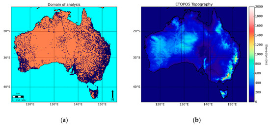
Figure 1.
Domain of analysis. (a) Stations are marked as blue dots; (b) scale of topography.
2.2. Datasets
As part of the WMO SEMDP, access to GSMaP and CMORPH data were provided by JAXA and NOAA, respectively. Both datasets of satellite precipitation estimates employ the cloud-advection technique introduced in Section 1. The GSMaP version used was GSMaP Gauge-adjusted Near-Real-Time (GNRT) Version 6. To allow for a faster data latency, gauge adjustment over land was performed against the gauge-calibrated version (GSMaP gauge) from the past period, which, itself, is calibrated by matching daily satellite rainfall estimates to a global gauge analysis, CPC Unified Gauge-Based Analysis of Global Daily Precipitation (CPC Unified) [28]. Further details can be found in the GSMaP technical documentation [28].
Two versions of CMORPH were used. These were the bias-corrected CMORPH (CMORPH CRT) and the gauge-blended CMORPH (CMORPH BLD) datasets. Bias correction over land was also performed using the CPC Unified analysis but using a different algorithm that involves matching to probability distribution function (PDF) tables from the past 30 days. The gauge-blended version uses the bias-corrected version as a first guess and then incorporates the gauge data based on the density of the observations; further details can be found in [10,13].
Consequently, this study used two gauge-corrected sets (GSMaP and CMORPH CRT) and one that had been further processed by combining CMORPH CRT with gauge data (CMORPH BLD).
The reference datasets used were both based on the Bureau of Meteorology (BoM) rain gauges with the Australian Water Availability Project (AWAP) analysis being used as the reference dataset for the gridded comparison and the values from the stations themselves being used for the point comparison. The AWAP rainfall analysis is generated by decomposing the field into a climatology component and an anomaly component based on the ratio of the observed rainfall value to the climatology [29]. The Barnes successive-correction technique is applied to the anomaly component and added to the monthly climatological averages, which were derived using a three-dimensional smooth splice approach [29]. The climatological averages were generated from 30 years of monthly totals [29]. For the point comparison, only ‘Series 0’ stations were chosen as these stations are Bureau-maintained and conform to International Civil Aviation Organization (ICAO) standards. The minimum number of stations used across the period was 4764. As discussed earlier, even though rain gauge network measurements can be taken as ‘truth’, they still contain errors, which will artificially inflate the errors attributed to satellite measurements.
Details on the spatial and temporal resolutions of the gridded datasets along with their domains are shown in Table 1.

Table 1.
Details about dataset used.
The longest common period across the datasets using full years was chosen for the analysis (i.e., January 2001 to December 2018). A spatial domain of latitude from −44.625°N to −10.125°N and longitude from 112.125°E to 156.125°E was chosen as this domain centers on Australia. Ocean data were masked.
2.3. Method
The satellite datasets were compared against the gauge-based datasets. Both a gridded comparison and point comparison were performed. When performing the comparisons, all the datasets were linearly interpolated to the same spatial resolution. An interpolation to the coarsest resolution was chosen (i.e., 0.25°). Values at each grid box from these interpolated grids could then be compared against each other for the gridded comparison.
For the point comparison, values corresponding to the location of a station were linearly interpolated from each grid. These values could then be compared to the actual station value. Inclusion of the AWAP dataset was done to provide an additional reference. A complication arose from the fact that the gauge-based data values were 24 h accumulated values to 0900 local standard time (LST), while the satellite data values were values to 00 UTC. As this study is focused on monthly comparisons, the longer period greatly reduces the impact of this timing inconsistency. An elementary remedy would be to have shifted the gauge and AWAP values one day ahead of their satellite counterparts, reducing the inconsistency to two hours or less. Doing this adjustment resulted in improvements of less than 2% and so the unadjusted datasets were used for simplicity.
Both continuous and percentile-based statistics were calculated. The continuous statistics calculated were the mean bias (MB), root-mean-square error (RMSE), mean average error (MAE), and the Pearson correlation coefficient (R). The MB is the average difference between the estimated and observed values, which gives an indicator of the overall bias. The MAE measures the average magnitude of the error. To remove the effect of higher rainfall averages leading to larger errors, the MAE was also normalised through division by the average rainfall producing the normalised mean average error. The RMSE also measures the average error magnitude but is weighted towards larger errors. R is commonly known as the linear correlation coefficient as it measures the linear association between the estimated and observed datasets.
In addition to continuous verification statistics, a percentile-based verification can also be performed to measure how well the datasets reproduce the occurrence of low- and high-end values. This is a novel verification metric that the authors have deemed useful to assess because, even if the satellites performs poorly in terms of absolute values, they may still produce accurate values relative to their own climatology, meaning there is the potential to produce percentile-based products. Such products have already been produced (e.g., both NOAA and JAXA have generated satellite-derived versions of the Standardized Precipitation Index, as well as rainfall values expressed as high-end percentiles). The quintile for an observed month at a location could be derived by ranking that value against the same month but for different years across the verification period. The ranking can then be converted to a percentile through linear interpolation. If a bottom or top quintile was observed, the value from the satellite dataset was then investigated. If it was also registered in the same quintile, this was recorded as a success; otherwise, it was recorded as a failure. The number of successes was then converted to a hit rate. This hit rate was only calculated for the gridded comparison as the varying number of stations across the verification period made a point-based comparison more difficult. The use of quintiles provided greater differentiation of extreme values than terciles or quartiles, while the record length was considered too short for the use of deciles.
The equations for the metrics are summarised in Table 2 with Ei representing the estimated value at a point or grid box i, Oi being the observed value, and N being the number of samples (across the whole domain and period) for the continuous metrics.
Table 2.
Summary of metrics used.
3. Results
The results of the gridded continuous comparison against AWAP data are presented in Figure 2. The linear correlation of the satellite rainfall estimates ranges from 0.77 to 0.88, while the MAE ranges from 0.61 to 0.43 mm/day. The trend amongst all the metrics is the same with performance being the best for CMORPH BLD, then CMORPH CRT, and lastly GSMaP. CMORPH CRT and GSMaP display similar performances, while there is a clear increase in performance for CMORPH BLD.
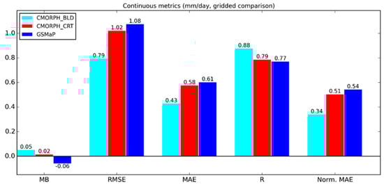
Figure 2.
Gridded continuous comparison of satellite datasets against Australian Water Availability Project (AWAP) from January 2001 to December 2018. Mean bias (MB), root-mean-square error (RMSE), mean average error (MAE), Pearson correlation coefficient (R) and normalised mean average error (Norm. MAE) are displayed.
The gridded percentile-based comparison against AWAP data is shown in Figure 3. The satellite datasets obtain around a 70%–80% hit rate for the bottom quintile whilst scoring around 10% less for the top quintile. This suggests the rainfall values produced by the satellites are relatively accurate in terms of climatological occurrence, with better performance exhibited for low-end extremes. There appears to be potential in generating percentile-based products from satellite data.
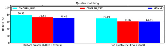
Figure 3.
Gridded percentile-based comparison of satellite datasets against AWAP from January 2001 to December 2018. Bottom- and top-quintile hit rates are displayed.
Figure 4 displays the continuous statistics using point gauge data as truth. The comparison against point gauge data supports the gridded comparison with the CMORPH BLD error being about 50% larger than the AWAP error and CMORPH CRT and GSMaP being about 150% larger. The MB is negative for all the satellite datasets, indicating a slight tendency for underestimation of overall rainfall.
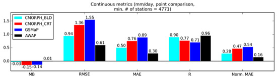
Figure 4.
Comparison of satellite datasets against point gauge data from January 2001 to December 2018.
The ranking of performance between the satellite datasets remains the same for both the continuous and the percentile-based statistics. The benefit of blending in gauge data is again displayed, with CMORPH BLD showing significant improvement over the unblended datasets and skill comparable to AWAP. As the trend between MB, MAE, RMSE, and R is the same, future references to continuous statistics will refer to just MAE, normalised MAE and R for brevity.
The values and residuals of the datasets against point gauge data are shown in Figure 5. There appears to be a tendency towards an overestimation for low rainfall months and an underestimation for high rainfall months. AWAP and, to a lesser extent, CMORPH BLD were able to capture the high-end rainfall months more accurately, with observation of months where more than 40 mm/day was recorded, being distinctly better. All datasets appear to struggle with very high-end rainfall months (>60 mm/day). These gauge totals sit along the lower boundary, which indicates that the datasets observed little rainfall while the gauges observed a significant amount. The fact that even AWAP does not depict these totals well suggests that gridded datasets systematically struggle with these very high-end values. A likely reason is that the gridded datasets smooth down point values as part of their objective analysis process and so it is expected that high-end totals will be underrepresented by the grids. The impact from this effect would be worse if there were nearby gauges with low totals.
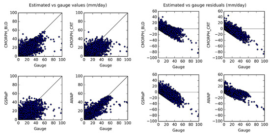
Figure 5.
Scatterplot comparisons of satellite datasets against point gauge data from January 2001 to December 2018.
3.1. Variation with Geography
A gridded comparison was performed over the Australian domain with the geographical representations of the MB and MAE shown in Figure 6. The CMORPH CRT and CMORPH BLD datasets were chosen to allow an investigation into the effects of gauge correction. Generally, the satellite-derived data overestimate rainfall, except over western Tasmania where there is a significant underestimation.
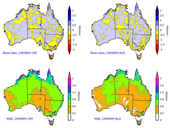
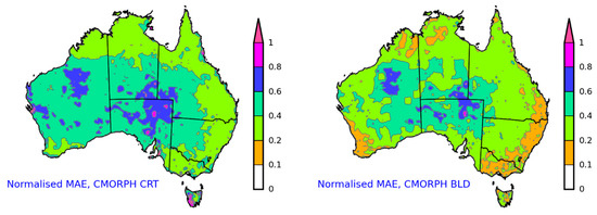
Figure 6.
Mean bias, mean average error, and normalised mean average error for bias-corrected Climate Prediction Center morphing technique (CMORPH CRT) and gauge-blended CMORPH (CMORPH BLD) datasets from January 2001 to December 2018 using AWAP as truth.
The effects of normalisation are indicated along the northern coast of Australia and in western Tasmania where the unnormalised errors were previously the greatest but improve to about average after the adjustment, at least for the CMORPH BLD dataset.
The effect of gauge correction is especially evident around western Tasmania, as well as around western parts of Western Australia, the southern Australian coastline, the northern coastline of New South Wales, the Australian Alps, and the southwestern coast of Western Australia. In these areas, there are significant improvements in the normalised errors from the uncorrected dataset to the corrected one, indicating that there is a problem with satellite rainfall detection that cannot be accounted for by higher rainfall averages. Possible reasons will be discussed in the next section.
A point-based comparison using rain gauges categorised by states supported the gridded comparison with the results shown in Figure 7. The unnormalised MAE values suggest that performance is decreased in the tropical regions and in Tasmania, but after normalisation, the performance is much more even across the states. The performance is slightly worse in Queensland and South Australia, while gauge correction appears to have the greatest effect in Tasmania.
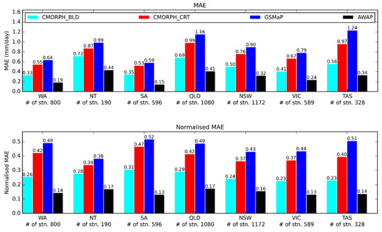
Figure 7.
Point-based comparison categorised by states from January 2001 to December 2018 using station gauges as truth.
3.2. Variation with Seasons
A seasonal analysis was completed by categorising the data into four seasons with December, January, and February (DJF); March, April, and May (MAM); June, July, and August (JJA); and September, October, and November (SON) representing austral summer, autumn, winter, and spring respectively.
A gridded comparison showing the normalised MAE from the CMORPH BLD dataset is displayed in Figure 8. The greatest seasonal variation of the error is observed towards the interior and around the northern coastline with winter possessing the worst performance and summer having the best.
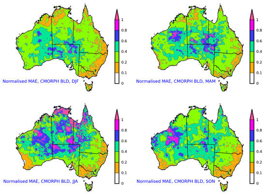
Figure 8.
Gridded comparison categorised by seasons from January 2001 to December 2018 using AWAP as truth. Normalised mean average error from CMORPH BLD is displayed.
An analysis using point gauge data was also performed with the results shown in Figure 9. The MAE is the smallest in SON and largest in DJF where the error is approximately 50% greater. Normalisation of the errors results in the smallest relative error occurring in DJF and the largest in MAM and JJA, supporting the gridded comparison. The linear correlation coefficients across the seasons also suggest that DJF has the best performance across the seasons. The performance increase is more prominent in the non-gauge blended datasets, where the improvement is at least 10%.
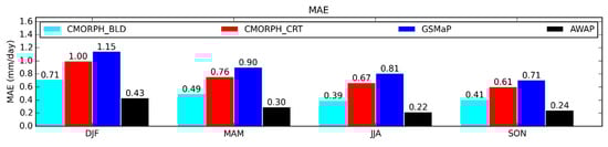
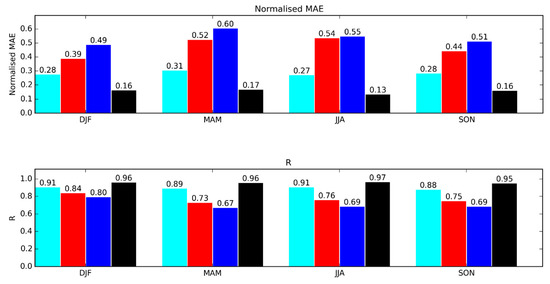
Figure 9.
Point-based comparison categorised by seasons from January 2001 to December 2018 using station gauges as truth. Mean average error (MAE), normalised MAE, and R are displayed.
Overall, the performance appears to be relatively similar across the seasons with the exception of DJF, which shows a somewhat superior performance to the rest.
3.3. Variations with Rainfall Intensity
The effects of the intensity of the rainfall on the accuracy of the data were also analysed. The data were categorised into these bins: 0–0.2, 0.2–1, 1–2, 2–3, 3–4, 4–6, 6–9, and >9 mm/day. These rainfall ranges were chosen to ensure there were a reasonable amount of values in each bin with the values of 0.2 and 1 mm being specifically chosen as they correspond to the rainy-day threshold for BoM and a commonly used value in contingency statistics studies, respectively [15]. Continuous statistics for these bins were calculated along with a comparison of occurrence frequencies and cumulative volumes. These are shown in Figure 10.
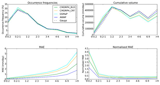
Figure 10.
Point-based comparison categorised by rainfall intensities from January 2001 to December 2018 using station gauges as truth. Occurrence frequencies, cumulative volumes, mean average error (MAE), and normalised MAE are displayed.
The datasets appear to capture the correct frequency best for rainfall amounts between 3 and 6 mm/day. For higher amounts, the satellite-derived data underestimate the frequency, while for lower amounts, the frequency is underestimated for very low values (<0.2 mm/day) but overestimated between the range of 0.2 and 3 mm/day. The change in sign of the bias from 0–0.2 to 0.2–1 mm/day may indicate that very-low-rainfall events are being incorrectly attributed to the higher ranges. For values above 1 mm/day, the frequency matches the gauge data quite well.
Analysis of the cumulative volumes demonstrates that below 1–3 mm/day, the satellite-derived data overestimate the gauge amount, while above this range, they underestimate the amount. Combining this result with the frequency analysis suggests that although the frequency of very-low-rainfall events is underestimated, each event is an overestimation of reality.
The MAE suggests decreasing skill as the rainfall rate increases. The normalised MAE was calculated by normalising the MAE by the mean rainfall amount for each bin. It indicates that the relative error was the largest for very small values (<0.2 mm/day).
Overall, satellite-derived data appears to be most reliable for low-moderate rainfall totals (2–4 mm/day), with a significant underestimation of amounts occurring for high-end totals and an underestimation of frequency and overestimation of amounts occurring for very low totals.
4. Discussion
It is important to acknowledge the effect of the errors in the reference datasets. The errors in the quality-controlled gauge network used for the point comparison are minor; however, the same cannot be said for the AWAP dataset used for the gridded comparison. Jones et al. (2009) performed a cross-validation of AWAP against station observations and found the monthly rainfall mean bias, RMSE, MAE, and normalised MAE to be 0.016, 0.7, 0.38, and 0.21 mm/day, respectively [29]. The RMSE and MAE for the satellite datasets ranged between 0.79 to 1.08 and 0.43 to 0.61 mm/day respectively, indicating that the errors in AWAP are comparable to those in the satellite datasets using AWAP as truth. To gain a better idea of the true error of the datasets, the satellite datasets along with AWAP were compared to a climate reanalysis (ERA5). A climate reanalysis is a numerical representation of meteorological fields created by combining meteorological observations with climate models. A gridded comparison using ERA5 as the reference was completed and is presented in Figure 11 and Figure 12. The results demonstrate comparable performance across the datasets. CMORPH BLD and AWAP displayed remarkably similar performances.
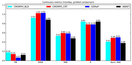
Figure 11.
Gridded comparison of satellite datasets and AWAP against ERA5 reanalysis from January 2001 to December 2018. Mean bias (MB), root-mean-square error (RMSE), mean average error (MAE), R and normalised MAE are displayed.
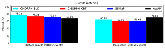
Figure 12.
Gridded comparison of satellite datasets and AWAP against ERA5 reanalysis from January 2001 to December 2018. Quintile comparison is displayed.
The results of the error analysis of the gridded comparison are supported by the point-based comparison where both satellite datasets and AWAP were compared to station gauges with the errors in AWAP being smaller but still within the same order of magnitude as those from the satellite dataset. This highlights the caution needed in understanding that the gridded comparison results are unlikely to be a proper depiction of the true error of the satellite datasets.
There are certain regions where the performance of satellite rainfall detection is decreased. Past studies have indicated that the detection of cold frontal-based rainfall is poor [15,17]. The absence of ice crystals in the relatively low precipitating clouds typically associated with frontal rainfall hinders the ability of satellites to detect rainfall via scattering [15]. This is a likely factor behind the large errors over Tasmania, Western Australia, South Australia, and central Australia, areas where the prevalent rainfall generation mechanism is cold frontal systems. Errors are pronounced over the western half of Tasmania and the southwestern coast of Western Australia, areas of relatively high rainfall due to increased exposure to westerly flow and associated cold fronts.
Performance is also known to be decreased over topography [18,21]. Decreased performance is observed along the eastern coastline near the Great Dividing Range. The errors are greatest along the northern NSW coastline and the Australian Alps where the Great Dividing Range is at its highest elevations, leading to a strong orographic influence on rainfall.
A high-quality rain gauge network is extremely valuable for improving the accuracy of satellite-derived rainfall estimates as satellite estimates rely on gauges to calibrate or correct their raw values. The significantly greater number of gauges towards the coastline where most of Australia’s population resides allows for a much greater improvement from gauge correction in contrast to the interior of the continent. Consequently, areas towards the coastlines that experience problematic regimes such as cold-frontal rainfall and orographically influenced rainfall greatly benefit from gauge correction, resulting in a performance similar to unproblematic regimes. However, the lack of rain gauges towards the interior means there are still large normalised errors in this region, even in the gauge-corrected dataset. This is compounded by the tendency of rainfall to be lighter towards the interior compared to the coast as light rainfall has been shown to be a problematic regime as well [17,18].
Low mean rainfall is another factor that would contribute to a large normalised MAE. Some areas of large normalised MAE around the interior of the continent can be seen to generally align with areas of low mean rainfall values, as seen in Figure 13, which depicts the seasonal mean rainfall across Australia. This is especially true during the austral winter ‘dry’ season for central Australia and northwards towards the Northern Territory coast.
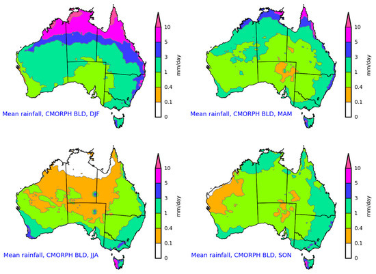
Figure 13.
Mean CMORPH BLD rainfall by season from January 2001 to December 2018.
The importance of gauge correction is reduced for unproblematic regimes. For example, the normalised errors for the corrected and uncorrected datasets around the northern coastline of Australia are relatively similar, highlighting how the raw satellite algorithms exhibit decent performance in these areas, leading to gauge correction being less crucial. Tropical-based rainfall has been noted to be one of the better-performing regimes for satellite rainfall detection [15].
Satellite-derived precipitation estimates for austral winter demonstrate the worst performance, a result that agrees with past studies [15]. The difficulty of detecting cold-frontal rainfall, which is more frequent during winter, is most likely a key factor. The introduction of snow is another challenge for satellite detection of precipitation and is likely a contributing factor to the poor performance observed in western Tasmania and the Australian Alps. By contrast, the greater prevalence of convective-based rainfall in summer is a reason for this season performing the best [15,17].
An overestimation (underestimation) of low (high) rainfall rates was observed and is consistent with past literature [19,20].
It is natural to expect that CMORPH BLD (a gauge-blended dataset) should have at least equal performance to AWAP (a gauge-based analysis) as it relies on using gauges where the data exist whilst depending more heavily on satellites where there is little to no gauge data. However, the key assumption here is that satellite depiction of rainfall is superior to interpolation methods in areas with little to no data. This is not necessarily true, as, even though satellites are sourcing their data through a physical sensor, this process still relies heavily on calibration to rain gauge data. For locations where there is little to no gauge data, calibration and, subsequently, performance will be severely hindered. Furthermore, AWAP used a minimum number of stations exceeding 3000 while the satellite datasets are calibrated to the CPC Unified gauge analysis, which has a minimum number of stations across Australia at least an order of magnitude less than that of AWAP [29,30]. The ingestion of less data is likely to contribute to the discrepancies observed.
5. Conclusions
The high spatial variation of rainfall along with the issue of installing a sufficiently dense network of rain gauges in many areas around the world make satellites an attractive option in terms of their ability to provide a continuous estimate of near-surface rainfall. Numerous verifications of satellite-estimated rainfall have been performed in the past, but few studies have focused on Australia using a relatively long data record. This study aimed to fill that gap by performing a validation over Australia using monthly CMORPH (both the bias-corrected CMORPH CRT and the gauge-blended CMORPH BLD) and GSMaP (gauge-corrected) data across an 18 year period from 2001 to 2018.
Station data were used as a point of reference, both in the form of the AWAP analysis along with individual stations in order to enable both a gridded and point-based comparison, respectively. Both continuous statistics (MB, MAE, RMSE, and R) and percentile-based statistics (hit rate for bottom and top quintiles) were chosen. General performance along with the geographical, seasonal, and intensity dependencies were subsequently investigated.
Overall statistics showed that satellite performance was decent and, in the case of CMORPH BLD, somewhat comparable to the AWAP analysis used as truth. CMORPH BLD performed best followed by CMORPH CRT and then GSMaP. Linear correlations from 0.71 to 0.90 and a bottom quintile hit rate from 70% to 80% were especially encouraging.
A geographical analysis of the error dependency was completed by plotting the gridded errors over Australia, as well as by breaking down the point comparison into states. Western Australia, western Tasmania, central Australia, and the Australian Alps displayed large errors in the uncorrected datasets. Orographically influenced rainfall and cold frontal rainfall have been identified as problematic regimes by past studies and are applicable to these regions. The blending of gauge data was beneficial, especially for regions that had problematic rainfall regimes. However, a dense rain gauge network is also needed for accurate calibration, and it is likely that the lack of rain gauges towards the interior of the continent was probably the reason why little to no improvement was seen in the gauge-blended dataset over these areas.
Categorising the results by seasons demonstrated that the performance was relatively similar across the seasons, with satellite-derived precipitation estimates in austral summer performing best and those in austral winter performing worst. A categorisation by rainfall intensity suggested that the performance was best for moderate rainfall amounts (2–4 mm/day). The frequency of high-end rainfall was captured well but the amount was severely underestimated while low-end rainfall amounts were overestimated.
The main results from this study agree with past literature reconciling the performance of satellite-derived precipitation estimates over Australia with those seen around other regions in the world. The results obtained in this study are generally better than past studies. For example, Jiang et al. (2016) evaluated CMORPH CRT and CMORPH BLD over China on a monthly time scale from 2000 to 2012 and obtained slightly lower correlation coefficients of 0.72 and 0.83 respectively [16]. Possible reasons may be that satellite technology has continued to improve over the years, as well as Australia having a relatively high-quality and dense rain gauge network that allows for improved performance of gauge correction and blending.
The study supported the finding that orographically influenced rainfall and cold frontal rainfall are problematic regimes for satellite rainfall detection. Advancement in the detection of these regimes would be very beneficial. Gauge-blending was shown to be a worthy process; however, its performance is strongly tied to the availability of high-quality rain gauge network data, which do not exist in many regions. Considering that one of, if not, the most valuable use of satellite rainfall monitoring is in areas without rain gauges, an accuracy that is dependent on gauge-blending should not be relied on. The unblended datasets do demonstrate skilful performance, which would be useful for areas that lack a rain gauge network, but there is still a considerable amount of progress needed to bring unblended datasets to a level comparable to that of rain gauges.
To conclude, evaluation of satellite precipitation estimates (CMORPH and GSMaP) is an essential scientific contribution to WMO activities in assisting countries in Asia and the Pacific with improving precipitation monitoring (including accumulated heavy precipitation and drought monitoring) which WMO provides through its flagship initiatives such as the Space-based Weather and Climate Extremes Monitoring [24] and the Climate Risk and Early Warning Systems [31], among others.
Author Contributions
Conceptualisation, Z.-W.C., Y.K. and A.W.; methodology, Z.-W.C. and Y.K.; software, Z.-W.C.; validation, Z.-W.C.; formal analysis, Z.-W.C.; writing—original draft preparation, Z.-W.C.; writing—review and editing, Z.-W.C., Y.K., A.W.; visualisation, Z.-W.C.; supervision, Y.K. and A.W.; funding acquisition, Y.K. All authors have read and agreed to the published version of the manuscript.
Funding
This research was funded by the World Meteorological Organization as part of the Climate Risk and Early Warning Systems (CREWS) international initiative.
Acknowledgments
GSMaP data were provided by EORC, JAXA. CMORPH data were provided by CPC, NOAA. AWAP and station gauge data were provided by the Bureau of Meteorology. Contains modified Copernicus Climate Change Service Information [2019]. Neither the European Commission nor ECMWF is responsible for any use that may be made of the Copernicus Information or Data it contains. William Wang and Elizabeth Ebert provided useful comments that helped us to improve the quality of the initial manuscript. We are grateful to colleagues from the Climate Monitoring and Long-range Forecasts sections of the Bureau of Meteorology for their helpful advice and guidance.
Conflicts of Interest
The authors declare no conflict of interest. The funders had no role in the design of the study; in the collection, analyses, or interpretation of data; in the writing of the manuscript, or in the decision to publish the results.
References
- WMO. Status of the Global Observing System for Climate; WMO: Geneva, Switzerland, 2015; p. 54. [Google Scholar]
- Kidd, C.; Becker, A.; Huffman, G.; Muller, C.; Joe, P.; Skofronick-Jackson, G.; Kirschbaum, D. So, how much of the Earth’s surface is covered by rain gauges? Bull. Amer. Meteor. Soc. 2017, 98, 69–78. [Google Scholar] [CrossRef]
- Michaelides, S.; Levizzani, V.; Anagnostou, E.; Bauer, P.; Kasparis, T.; Lane, J.E. Precipitation: Measurement, remote sensing, climatology and modeling. Atmos. Res. 2009, 94, 512–533. [Google Scholar] [CrossRef]
- Michelson, D. Systematic correction of precipitation gauge observations using analyzed meteorological variables. J. Hydrol. 2004, 290, 161–177. [Google Scholar] [CrossRef]
- Peterson, T.; Easterling, D.; Karl, T.; Groisman, P.; Nicholls, N.; Plummer, N.; Torok, S.; Auer, I.; Boehm, R.; Gullett, D.; et al. Homogeneity adjustments of in situ atmospheric climate data: A review. Int. J. Climatol. 1998, 18, 1493–1517. [Google Scholar] [CrossRef]
- Groisman, P.; Legates, D. The accuracy of United States precipitation data. Bull. Amer. Meteor. Soc. 1994, 75, 215–227. [Google Scholar] [CrossRef]
- Young, C.; Bradley, A.; Krajewski, W.; Kruger, A.; Morrissey, M. Evaluating NEXRAD Multisensor Precipitation Estimates for Operational Hydrologic Forecasting. J. Hydrometeor. 2000, 1, 241–254. [Google Scholar] [CrossRef]
- Krajewski, W.; Smith, J. Radar hydrology: Rainfall estimation. Adv. Water Resour. 2002, 25, 1387–1394. [Google Scholar] [CrossRef]
- Beek, C.; Leijnse, H.; Hazenberg, P.; Uijlenhoet, R. Close-range radar rainfall estimation and error analysis. Atmos. Meas. Tech. 2016, 9, 3837–3850. [Google Scholar] [CrossRef]
- Joyce, R.; Janowiak, J.; Arkin, P.; Xie, P. CMORPH: A Method that Produces Global Precipitation Estimates from Passive Microwave and Infrared Data at High Spatial and Temporal Resolution. J. Hydrometeor. 2004, 5, 487–503. [Google Scholar] [CrossRef]
- Okamoto, K.; Ushio, T.; Iguchi, T.; Takahashi, N.; Iwanami, K. The Global Satellite Mapping of Precipitation (GSMaP) project. In Proceedings of the International Geoscience and Remote Sensing Symposium (IGARSS), Seoul, Korea, 14 November 2005. [Google Scholar] [CrossRef]
- Ushio, T.; Kachi, M. Kalman filtering applications for global satellite mapping of precipitation (GSMaP). In Satellite Rainfall Applications for Surface Hydrology; Springer: Dordrecht, The Netherlands, 2010; pp. 105–123. [Google Scholar] [CrossRef]
- Xie, P.; Joyce, R.; Wu, S.; Yoo, S.; Yarosh, Y.; Sun, F.; Lin, R. Reprocessed, bias-corrected CMORPH global high-resolution precipitation estimates from 1998. J. Hydrometeor. 2017, 18, 1617–1641. [Google Scholar] [CrossRef]
- Jiang, S.; Zhou, M.; Ren, L.; Cheng, X.; Zhang, P. Evaluation of latest TMPA and CMORPH satellite precipitation products over Yellow River Basin. Water Sci. Eng. 2016, 9, 87–96. [Google Scholar] [CrossRef]
- Ebert, E.; Janowiak, J.; Kidd, C. Comparison of near-real-time precipitation estimates from satellite observations and numerical models. Bull. Amer. Meteor. Soc. 2007, 88, 47–64. [Google Scholar] [CrossRef]
- Xu, R.; Tian, F.; Yang, L.; Hu, H.; Lu, H.; Hou, A. Ground validation of GPM IMERG and TRMM 3B42V7 rainfall products over Southern Tibetan plateau based on a high-density rain gauge network. J. Geophys. Res. 2017, 122, 910–924. [Google Scholar] [CrossRef]
- Pipunic, R.; Ryu, D.; Costelloe, J.; Su, C. An evaluation and regional error modeling methodology for near-real-time satellite rainfall data over Australia. J. Geophys. Res. 2015, 120, 10767–10783. [Google Scholar] [CrossRef]
- Dinku, T.; Ceccato, P.; Grover-Kopec, E.; Lemma, M.; Connor, S.; Ropelewski, C. Validation of satellite rainfall products over East Africa’s complex topography. Int. J. Remote Sens. 2007, 28, 1503–1526. [Google Scholar] [CrossRef]
- Habib, E.; Haile, A.; Tian, Y.; Joyce, R. Evaluation of the High-Resolution CMORPH Satellite Rainfall Product Using Dense Rain Gauge Observations and Radar-Based Estimates. J. Hydrometeor. 2012, 13, 1784–1798. [Google Scholar] [CrossRef]
- Ning, S.; Song, F.; Udmale, P.; Jin, J.; Thapa, B.; Ishidaira, H. Error Analysis and Evaluation of the Latest GSMap and IMERG Precipitation Products over Eastern China. Adv. Meteorol. 2017, 2017, 1–16. [Google Scholar] [CrossRef]
- Derin, Y.; Yilmaz, K. Evaluation of multiple satellite-based precipitation products over complex topography. J. Hydrometeor. 2014, 15, 1498–1516. [Google Scholar] [CrossRef]
- Stampoulis, D.; Anagnostou, E. Evaluation of global satellite rainfall products over Continental Europe. J. Hydrometeor. 2012, 13, 588–603. [Google Scholar] [CrossRef]
- Kubota, T.; Ushio, T.; Shige, S.; Kida, S.; Kachi, M.; Okamoto, K. Verification of high-resolution satellite-based rainfall estimates around japan using a gauge-calibrated ground-radar dataset. J. Meteorol. Soc. Jpn. 2009, 87, 203–222. [Google Scholar] [CrossRef]
- Kuleshov, Y.; Kurino, T.; Kubota, T.; Tashima, T.; Xie, P. WMO Space-based Weather and Climate Extremes Monitoring Demonstration Project (SEMDP): First Outcomes of Regional Cooperation on Drought and Heavy Precipitation Monitoring for Australia and Southeast Asia. In Rainfall—Extremes, Distribution and Properties; IntechOpen: London, UK, 2019; pp. 51–57. [Google Scholar] [CrossRef]
- Beck, H.; Vergopolan, N.; Pan, M.; Levizzani, V.; van Dijk, A.; Weedon, G.; Brocca, L.; Pappenberger, F.; Huffman, G.; Wood, E. Global-scale evaluation of 22 precipitation datasets using gauge observations and hydrological modeling. Hydro. Earth Syst. Sci. 2017, 21, 6201–6217. [Google Scholar] [CrossRef]
- Beck, H.; Zimmermann, N.; McVicar, T.; Vergopolan, N.; Berg, A.; Wood, E. Present and future köppen-geiger climate classification maps at 1-km resolution. Sci. Data 2018, 5, 180214. [Google Scholar] [CrossRef] [PubMed]
- Johnson, D. The Geology of Australia, 2nd ed.; Cambridge University Press: Cambridge, UK, 2009; p. 202. [Google Scholar] [CrossRef]
- Global Satellite Mapping of Precipitation (GSMaP) for GPM Algorithm Theoretical Basis Document Version 6. Available online: https://eorc.jaxa.jp/GPM/doc/algorithm/GSMaPforGPM_20140902 (accessed on 14 September 2019).
- Jones, D.; Wang, W.; Fawcett, R. High-quality spatial climate data-sets for Australia. Aust. Meteorol. Ocean. 2009, 58, 233–248. [Google Scholar] [CrossRef]
- Chen, M.; Shi, W.; Xie, P.; Silva, V.; Kousky, V.; Higgins, R.; Janowiak, J. Assessing objective techniques for gauge-based analyses of global daily precipitation. J. Geophys. Res. 2008, 113, D4. [Google Scholar] [CrossRef]
- Kuleshov, Y.; Inape, K.; Watkins, A.B.; Bear-Crozier, A.; Chua, Z.-W.; Xie, P.; Kubota, T.; Tashima, T.; Stefanski, R.; Kurino, T. Climate Risk and Early Warning Systems (CREWS) for Papua New Guinea. In Drought–Detection and Solutions; IntechOpen: London, UK, 2020; pp. 147–168. [Google Scholar] [CrossRef]
© 2020 by the authors. Licensee MDPI, Basel, Switzerland. This article is an open access article distributed under the terms and conditions of the Creative Commons Attribution (CC BY) license (http://creativecommons.org/licenses/by/4.0/).